The Compute-and-Forward Protocol: Implementation and Practical Aspects

Abstract

In a recent work, Nazer and Gastpar proposed the Compute-and-Forward strategy as a physical-layer network coding scheme. They described a code structure based on nested lattices whose algebraic structure makes the scheme reliable and efficient. In this work, we consider the implementation of their scheme for real Gaussian channels and one dimensional lattices. We relate the maximization of the transmission rate to the lattice shortest vector problem. We explicit, in this case, the maximum likelihood criterion and show that it can be implemented by using an Inhomogeneous Diophantine Approximation algorithm.

I Introduction

In [1], Zhang et al. introduced the physical-layer network coding concept (PNC) in order to turn the broadcast property of the wireless channel into a capacity boosting advantage. Instead of considering the interference as a nuisance, each relay converts an interfering signal into a combination of simultaneously transmitted codewords. PNC concept has received a particular interest in the last years because it provides means of embracing interference and improving network capacity.

In a recent work [2], Nazer and Gastpar proposed a new physical-layer network coding scheme. Their strategy, called compute-and-forward (CF), exploits interference to obtain higher end-to-end transmission rates between users in a network. The relays are required to decode noiseless linear equations of the transmitted messages using the noisy linear combination provided by the channel. The destination, given enough linear combinations, can solve the linear system for its desired messages. This strategy is based on the use of structured codes, particularly nested lattice codes to ensure that integer combinations of codewords are themselves codewords. The authors demonstrated its asymptotic gain using information-theoretic tools.

The authors in [3] followed the framework of Nazer and Gastpar and showed the potential of the compute-and-forward protocol using an algebraic approach. They related the Nazer-Gastaper’s approach to the theorem of finitely generated modules over a principle ideal domain (PID). They gave sufficient condition for lattice partitions to have a vector space structure which is a desirable property to make them well suited for physical-layer network coding. Then, they generalized the code construction and developed encoding and decoding methods.

In [4], the authors proved that the lattice implementation of compute-and-forward as proposed by Nazer and Gastpar suffers from a loss in number of achieved degrees of freedom. They proposed a different implementation consisting of a modulation scheme and an outer code and showed that it achieves full degrees of freedom as if full cooperation among transmitters and among relays was permitted. In their scheme, the channel coefficients are known throughout the network. In [5], the authors designed a modulation/coding scheme inspired by the compute-and-forward protocol for the wireless two-way relaying channel.

In this work, we consider the practical aspects of the compute-and-forward protocol. We implement the protocol described by Nazer and Gastpar. We explain how to obtain the integer coefficients that maximize the rate. We also propose a decoding technique based on maximum likelihood. Finally, we show some simulation results. All the practical aspects are demonstrated here for one-dimensional real constellations.

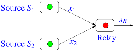
Figure 1: System model: 2 sources and one relay.

II System Model and Assumptions

In our model, we consider one relay receiving messages from two sources $S_{1}$ and $S_{2}$ and transmitting a linear combination of these two messages, as described in Figure 1. The relay observes a noisy linear combination of the transmitted signals through the channel. Received signal at the relay is expressed as,

$$y=h_{1}x_{1}+h_{2}x_{2}+z.$$ (1)

The relay searches for the integer coefficient vector $\boldsymbol{a}=[a_{1}\hskip 2.84544pta_{2}]^{T}$ that maximizes the transmission rate. It then decodes a noiseless linear combination of the transmitted signals,

$$x_{R}=a_{1}x_{1}+a_{2}x_{2},$$ (2)

and retransmits it to the destination or another relay. We consider a real-valued channel model with real inputs and outputs. The channel coefficients $h_{1}$ and $h_{2}$ are real, i.i.d. Gaussian, $h_{i}\sim\mathcal{N}(0,1)$. $z$ is Gaussian, zero mean, with variance $\sigma^{2}=1$ ($z\sim\mathcal{N}(0,1)$). Let $\boldsymbol{h}=[h_{1}\hskip 2.84544pth_{2}]^{T}$ denotes the vector of channel coefficients. Source symbols $x_{i}$ are integers and verify $\lvert x_{i}\rvert\leq s_{m}$, i.e., $x_{i}\in\mathcal{S}=\left\{-s_{m},-s_{m}+1,\ldots,s_{m}\right\}$. $S_{1}$ and $S_{2}$ transmit $x_{1}$ and $x_{2}$, respectively. Both sources have no channel side information (CSI). CSI is only available at the relay.

III Compute-and-Forward

In what follows, we use the expression of the computation rate $R_{\mathrm{comp}}$ given by Nazer and Gastpar [2] in order to find a vector $\boldsymbol{a}$ maximizing it. We show that the maximization of $R_{\mathrm{comp}}$ is equivalent to the search of a shortest vector in a lattice. Then, based on the likelihood expression, we show that decoding is equivalent to an Inhomogeneous Diophantine Approximation.

III-A Achievable Computation Rate

The primary goal of the decode-and-forward is to enable higher achievable rates across the network. Nazer and Gastpar showed that the relays can recover any set of linear equations with coefficient vector $\boldsymbol{a}$ as long as the message rates are less than the computation rate

$$R_{\mathrm{comp}}(\boldsymbol{h},\boldsymbol{a})=\log\left(\left(\lVert\boldsymbol{a}\rVert^{2}-\dfrac{\mathsf{SNR}\lvert\boldsymbol{h}^{\dagger}\boldsymbol{a}\rvert^{2}}{1+\mathsf{SNR}\lVert\boldsymbol{h}\rVert^{2}}\right)^{-1}\right)$$ (3)

where this rate is achievable by scaling the received signal by the MMSE coefficient [2]. We are interested in finding the coefficient vector with the highest computation rate. This is given in the following theorem. The result is obtained for a relay combining $N$ symbols and for complex-valued channels.

Theorem 1

For a given $\boldsymbol{h}\in\mathbb{C}^{N}$ (resp. $\mathbb{R}^{N}$), $R_{\mathrm{comp}}(\boldsymbol{h},\boldsymbol{a})$ is maximized by choosing $\boldsymbol{a}\in\mathbb{Z}[i]^{N}$ (resp. $\mathbb{Z}^{N}$) as

$$\boldsymbol{a}=\arg\min\limits_{\boldsymbol{a}\neq\boldsymbol{0}}\left(\boldsymbol{a}^{\dagger}\boldsymbol{G}\boldsymbol{a}\right)$$ (4)

where

$$\boldsymbol{G}=\boldsymbol{I}-\dfrac{\mathsf{SNR}}{1+\mathsf{SNR}\lVert\boldsymbol{h}\rVert^{2}}\boldsymbol{H}.$$ (5)

$\boldsymbol{H}=[H_{ij}]$, $H_{ij}=h_{i}h_{j}^{\star}$, $1\leq i,j\leq N$ and $\dagger$ is for the Hermitian transpose (resp. the regular transpose).

Proof:

Maximizing $R_{\mathrm{comp}}(\boldsymbol{h},\boldsymbol{a})$ is equivalent to the following minimization

$$\min\limits_{\boldsymbol{a}\neq\boldsymbol{0}}\left\{\lVert\boldsymbol{a}\rVert^{2}+\mathsf{SNR}\lVert\boldsymbol{h}\rVert^{2}\lVert\boldsymbol{a}\rVert^{2}-\mathsf{SNR}\lvert\boldsymbol{h}^{\dagger}\boldsymbol{a}\rvert^{2}\right\}.$$ (6)

We can write

$$\lvert\boldsymbol{h}^{\dagger}\boldsymbol{a}\rvert^{2}=\sum\limits_{i,j}h_{i}h_{j}^{\star}a_{i}^{\star}a_{j}$$ (7)

As $\boldsymbol{H}=[H_{ij}]$, $H_{ij}=h_{i}h_{j}^{\star}$, $1\leq i,j\leq N$, it follows that $\sum\limits_{i,j}h_{i}h_{j}^{\star}a_{i}^{\star}a_{j}=\boldsymbol{a}^{\dagger}\boldsymbol{H}\boldsymbol{a}$. Using these notations, we can write (6) as

$$(1+\mathsf{SNR}\lVert\boldsymbol{h}\rVert^{2})\min\limits_{\boldsymbol{a}\neq\boldsymbol{0}}\boldsymbol{a}^{\dagger}\left[\boldsymbol{I}-\dfrac{\mathsf{SNR}}{1+\mathsf{SNR}\lVert\boldsymbol{h}\rVert^{2}}\boldsymbol{H}\right]\boldsymbol{a}.$$ (8)

$\boldsymbol{I}-\dfrac{\mathsf{SNR}}{1+\mathsf{SNR}\lVert\boldsymbol{h}\rVert^{2}}\boldsymbol{H}$ has $N$ strictly positive eigenvalues. It is then positive definite. Now, the problem is reduced to the minimization of $\boldsymbol{a}^{\dagger}\boldsymbol{G}\boldsymbol{a}$. ∎

Proposition 1

Searching for the vector $\boldsymbol{a}$ that minimizes Equation (4) of theorem 1 is equivalent to a “Shortest Vector” problem for the lattice $\Lambda$ whose Gram matrix is $\boldsymbol{G}$.

Proof:

As $\boldsymbol{G}$ is a definite positive hermitian (resp. symmetric) matrix, it is the Gram matrix of a lattice $\Lambda$. This lattice is either a $\mathbb{Z}[i]-$ lattice in the complex case, or a $\mathbb{Z}-$ lattice in the real case. Then, the minimization problem in theorem 1 is equivalent to find a non zero vector in $\Lambda$ with shortest length. ∎

Algorithms for solving this problem are given in [6]. The best known one is the Fincke-Pohst algorithm [7].

III-B Recovering Linear Equations

The relay aims to decode a linear equation of the transmitted messages and passes it to the destination or another relay. After calculating the vector $\boldsymbol{a}$ as in (4), the relay recovers a linear combination of the transmitted signal $x_{1}$ and $x_{2}$. We rewrite the received signal at the relay in the following form

$$y=\lambda+\xi_{1}x_{1}+\xi_{2}x_{2}+z$$ (9)

where $\lambda$ is an integer, $\xi_{i}=h_{i}-a_{i}$ and $z$ is the additive white noise. The recovered linear equation $\lambda=a_{1}x_{1}+a_{2}x_{2}$ is a linear Diophantine equation. This equation admits the following solutions.

III-C Solution of the Linear Diophantine Equation

If $\lambda$ is a multiple of the greatest common divisor (gcd) of $a_{1}$ and $a_{2}$, then the Diophantine equation has an infinite number of solutions. The Extended Euclid Algorithm allows to exhibit a particular solution $(u_{1},u_{2})$ to $a_{1}x_{1}+a_{2}x_{2}=g$ [9]. The set of all solutions is obtained as follows

$$\begin{cases}x_{1}=\frac{u_{1}}{g}\lambda+\frac{a_{2}}{g}k\\ x_{2}=\frac{u_{2}}{g}\lambda-\frac{a_{1}}{g}k\end{cases}$$ (10)

$g=a_{1}\wedge a_{2}$ is the gcd of $a_{1}$ and $a_{2}$, $k\in\mathbb{Z}$.

III-D Decoding Metric

The Maximum Likelihood decoder maximizes $p(y/\lambda)$ over all possible values of $\lambda$. The conditional probability $p(y/\lambda)$ can be expressed as,

$$p(y/\lambda)=\sum_{\underset{a_{1}x_{1}+a_{2}x_{2}=\lambda}{(x_{1},x_{2})}}p(y/x_{1},x_{2})p(x_{1},x_{2})$$ (11)

where

$$p(y/x_{1},x_{2})\propto\exp\left[-\frac{(y-h_{1}x_{1}-h_{2}x_{2})^{2}}{2\sigma^{2}}\right]$$ (12)

and $x_{1}$, $x_{2}$ are (a priori) equiprobable and given by (10). The decoding rule is now to find,

$$\hat{\lambda}=\arg\max\limits_{\lambda}\varrho(\lambda):=\sum\limits_{k=-\infty}^{+\infty}\exp\left[-\frac{(y-\beta\lambda+k\alpha)^{2}}{2\sigma^{2}}\right]$$ (13)

where $\beta=\frac{1}{g}\left(h_{1}u_{1}+h_{2}u_{2}\right)$, $\alpha=\frac{1}{g}\left(h_{2}a_{1}-h_{1}a_{2}\right)$.

In [8], it has been proved that, for $\lambda\in\mathbb{R}$, $\varrho(\lambda)$ achieves its maximum for

$$\lambda\in\frac{\alpha}{\beta}\mathbb{Z}+\frac{y}{\beta},$$

i.e. for all values of $\lambda$ such that $y-\beta\lambda+k\alpha=0$. Since we want to maximize $\varrho(\lambda)$ for $\lambda\in\mathbb{Z}$, the solution is given by the integer-valued couple $(\lambda,k)$ minimizing $\left|y-\beta\lambda+k\alpha\right|$. Thus, since $x_{1},x_{2}\in\mathcal{S}$ which is a finite subset of $\mathbb{Z}$ and verify Equation (10), we state a new minimization problem which is equivalent to (13),

$$\hat{\lambda}=\arg\limits_{\lambda}\min_{\underset{x_{1},x_{2}\in\mathcal{S}}{(\lambda,k)}}\left|y-\beta\lambda+k\alpha\right|.$$ (14)

The problem is therefore equivalent to the minimization of

$$F(k,\lambda)=\left|k\alpha^{\prime}-\lambda+y^{\prime}\right|$$ (15)

$\alpha^{\prime}=\alpha/\beta$ and $y^{\prime}=y/\beta$. The minimization is called Inhomogeneous Diophantine Approximation in the absolute sense. It consists of finding the best approximation of a real number $\alpha^{\prime}$ by a rational number $\lambda/k$, $k$ $\in$ $\mathbb{N}$, given an additional real shift $y^{\prime}$, while keeping the denominator $k$ as small as possible. In the general settings for such problems, an error approximation function $F(k,\lambda)$ is set and it is stated that a rational number $\lambda/k$ is the Best Diophantine Approximation if, for all other rational numbers $\lambda^{\prime}/k^{\prime}$

$$k^{\prime}\leq k\Rightarrow F(k^{\prime},\lambda^{\prime})\geq F(k,\lambda).$$ (16)

In our case, in addition to the error approximation function, limits are imposed by the finite constellation $\mathcal{S}$ to which the transmitted symbols belong. The algorithms used to find the best Diophantine approximations of real numbers are in general simple and easy to implement. The best known one is the Cassel’s algorithm [10]. In [11], the authors develop and compare several ones.

IV Numerical Results

In the simulations, the set of symbols is of the form $\mathcal{S}=\left\{-s_{m},\ldots,s_{m}\right\}$. We consider two sources transmitting $x_{1}$ and $x_{2}$, and one relay recovering a linear equation of $x_{1}$ and $x_{2}$ with integer coefficients.

At first, based on its CSI, the relay finds the vector $\boldsymbol{a}$ as the shortest vector described in theorem 1. Then, the relay finds a particular solution of the linear Diophantine equation $a_{1}x_{1}+a_{2}x_{2}=g$ using the Extended Euclid algorithm. Finally, the relay searches for the couple $(k,\lambda)$ which gives the best inhomogeneous Diophantine approximation by minimizing the function $F$ defined in (15).

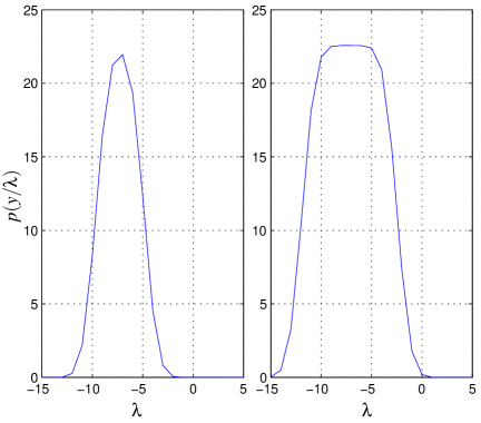
Figure 2: $p(y/\lambda)$ for $\boldsymbol{h}=[-1.274\hskip 2.84544pt0.602]^{T}$, $\boldsymbol{a}=[2\hskip 2.84544pt-1]^{T}$, $\mathsf{SNR}=40dB$, $x_{1}=-2$ and $x_{2}=3$. $p(y/\lambda)$ is maximized for one value, $\lambda=-7$ in the left subfigure while it is maximized for several values of $\lambda$ in the right one.

In Figure 3, we show the error probability of our system for three different constellations $\mathcal{S}$, defined by $s_{m}=5,7,10$, respectively. For $s_{m}=5$ or less, the diversity order of the system is 1 for real entries (which would correspond to a diversity order equal to 2 with complex symbols). For $s_{m}>6$, the diversity order collapses to $1/2$.

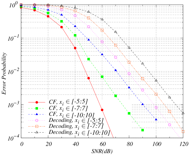
Figure 3: Error Probability using the Inhomogeneous Diophantine Approximation versus decoding both symbols $x_{1}$ and $x_{2}$.

This is due to the fact that $p(y/\lambda)$ is constant, as a function of $\lambda$, on a bigger interval giving rise to ambiguities as shown in Figure 2. Still in Figure 3, we plotted the error probability for when the relay decodes both symbols $x_{1}$ and $x_{2}$. The diversity order in this case is $1/2$ for all values of $s_{m}$. For the case of complex-valued channels and symbols, we expect a doubled value of all the diversity orders.

V Conclusion

In this paper, we considered the Compute-and-Forward scheme with real-valued channels. We provided a method for maximizing the transmission rate and developed a decoding strategy. Numerical results showed the performance of our decoding method. We believe that it is a first step towards a rich and fruitful multidimensional approach.

References

- [1] S. Zhang, S. Liew and P. Lam, “Physical Layer Network Coding,” in Proc. of ACM MOBICOM, Los Angeles, USA, 2006, available on http://arxiv.org/abs/0704.2475.
- [2] B. Nazer and M. Gastpar, “Compute-and-Forward: Harnessing Interference through Structured Codes,” submitted to IEEE Trans. on Inf. Th., available on http://arxiv.org/abs/0908.2119, Aug. 2009.
- [3] C. Feng, D. Silva and F. R .Kschischang ”An Algebraic Approach to Physical-Layer Network Coding,” in proceeding of ISIT 2010, available on http://arxiv.org/abs/1005.2646, May 2010.
- [4] U. Niesen and P. Whiting ”The Degrees of Freedom of Compute-and-Forward,” available on http://arxiv.org/abs/1101.2182, Jan 2011.
- [5] B. Hern and K. Narayanan ”Multilevel Coding Schemes for Compute-and-Forward,” available on http://arxiv.org/abs/1010.1016, Oct 2010.
- [6] H. Cohen ”A Course in Computational Algebraic Number Theory,” Springer-Verlag, 1993. Pages 103-105. Section 2.7.3: Finding Small Vectors in Lattices.
- [7] U. Fincke and M. Pohst ”Improved Methods for Calculating Vectors of Short Length in a Lattice, Including a Complexity Analysis,” Math. Comp. 44 (1985), 463-471.
- [8] D. Micciancio and O. Regev, “Worst-case to average-case reductions based on Gaussian measure,” SIAM J. on Computing, 37(1):267-302 (May 2007).
- [9] T. H. Cormen, C. E. Leiserson, R. L. Rivest and C. Stein ”Introduction to Algorithms,” Third Edition. The MIT Press, 2009. Pages 933-939. Section 31.2: Greatest Common Divisor
- [10] J. W. S. Cassels (1957) ”An Introduction to Diophantine Approximation”. Cambridge University Press.
- [11] I. V. L. Clarkson ”Approximation of Linear Forms by Lattice Points with Applications to Signal Processing,” thesis dissertation, January 1997.