A comparative study of Gaussian Graphical Model approaches for genomic data

Abstract

The inference of networks of dependencies by Gaussian Graphical models on high-throughput data is an open issue in modern molecular biology. In this paper we provide a comparative study of three methods to obtain small sample and high dimension estimates of partial correlation coefficients: the Moore-Penrose pseudoinverse (PINV), residual correlation (RCM) and covariance-regularized method $(\ell_{2C})$. We first compare them on simulated datasets and we find that PINV is less stable in terms of AUC performance when the number of variables changes. The two regularized methods have comparable performances but $\ell_{2C}$ is much faster than RCM. Finally, we present the results of an application of $\ell_{2C}$ for the inference of a gene network for isoprenoid biosynthesis pathways in Arabidopsis thaliana.

I Introduction

One of the aims of systems biology is to provide quantitative models for the study of complex interaction patterns among genes and their products that are the result of many biological processes in the cell, such as biochemical interactions and regulatory activities. In this framework, graphical models Lauritzen_book have been exploited as useful stochastic tools to investigate and describe the conditional independence structure between random variables. In particular, the Graphical Gaussian Models (GGM) use the partial correlation estimates as a measure of conditional independence between any two variables Dempster1972 . Unfortunately, the application of GGMs classical theory is still a hard task. The genomic data are tipically characterized by a huge number of genes $p$ with respect to the small number of available samples $n$. This makes unreliable the application of the classical GGMs theory to the small sample setting case. In recent years, several methods have been proposed to overcome this problem by reducing the numbers of genes or gene lists in order to reach the $n>p$ regime Toh2002 . Other solutions have been also proposed Wille2004 ; Castelo2006 ; Gilbert2009 to circumvent the problem of computing full partial correlation coefficients by using only zero and first order coefficients. However, these approaches do not take into account all multigene effects on each pair of variables. A more sophisticated way to adapt GGMs to the $n<p$ case is to find regularized estimates for the covariance matrix Yuan2007 ; Friedman2008 ; Witten2009 and its inverse. Once regularized estimates of partial correlation are available, heuristic searches can be used to find an optimal graphical model. A fundamental assumption to perform these quantitative methods is the sparsity of biological networks: only a few edges are supposed to be present in the gene regulatory networks, so that reliable estimates of the graphical model can be inferred also in small sample case Castelo2006 . A regularized GGM method based on a Stein-type shrinkage has been applied to genomic data Dobra2004 and the network selection has been based on false discovery rate multiple testing. In Ref. Schaffer2005 the same procedure to select the network has been adopted, with a Moore-Penrose pseudoinverse method to obtain the concentration matrix. Finally, the authors in Ref. Meinshausen2006 have suggested an attractive and simple approach based on lasso-type regression to select among the partial correlations the nonzero values, paving the way to a number of analysis and novel algorithms based on lasso $\ell_{1}$ regularizations Yuan2007 ; Friedman2008 ; Witten2009 ; Friedman2010 . In this work, we focus on regularized methods for the estimation of the concentration matrix in an undirected GGM. In particular, we present a comparative study of three methods in terms of AUC (area under the Receiving Operative Characteristic curve) and timing performances. One is based on Moore–Penrose pseudoinverse (PINV), the other two provide an estimate of the partial correlation coefficients, based on Regularized Least Square regression (RCM) and a covariance-regularized method with a $\ell_{2}$ penalty in the log-likelihood function $(\ell_{2C})$. Finally, we apply the $\ell_{2C}$ method to infer a gene network for the isoprenoid biosynthesis pathways in A. thaliana. This network structural analysis allows to enlight some expected pathway properties. In particular, we find a negative partial correlation coefficient between the two hubs in the two isoprenoid pathways. This suggests a different response of the pathways to the several tested experimental conditions and, together with the high connectivity of the two hubs, provides an evidence of cross-talk between genes in the plastidial and the cytosolic pathways.

II Gaussian networks from microarray data

Let ${\bf X}=(X_{1},\dots,X_{p})\in\mathbb{R}^{p}$ be a random vector distributed according a multivariate normal distribution $\mathcal{N}({\bm{\mu}},{\bm{\Sigma}})$. The interaction structure between these variables can be described by means of a graph $G=(V,E)$, where $V$ is the vertex set and $E$ is the edge set. If vertices of $V$ are identified with the random variables $X_{1},\dots,X_{p}$, then the edges of $E$ can represent the conditional dependence between the vertices. In other words, the absence of an edge between the $i-$th and $j-$th vertex means a conditional independence between the associated variables $X_{i}$ and $X_{j}$. In this study, we shall consider only undirected Gaussian graphs $G$ with pairwise Markov property, such that for all $(i,j)\notin E$ one has

$$X_{i} \perp\!\!\!\!\perp X_{j}\;|\;X_{V\backslash\{i,j\}} i,j =1,\dots,p\,,$$ (1)

i.e. $X_{i}$ and $X_{j}$ are conditionally independent being fixed all other variables $X_{V\backslash\{i,j\}}$. Since ${\bf X}$ follows a $p-$variate normal distribution, the condition (1) turns out to be $\rho_{ij\cdot V\backslash\{i,j\}}=0$, where $\rho_{ij\cdot V\backslash\{i,j\}}$ is the partial correlation coefficient between the $i-$th and $j-$th variable, being fixed all other variables. It has been shown Lauritzen_book that partial correlation matrix elements are related to the precision matrix (or inverse covariance matrix) $\bm{\Theta}=\bm{\Sigma}^{-1}$, as:

$$\rho_{ij\cdot V\backslash\{i,j\}}=-\frac{\theta_{ij}}{\sqrt{\theta_{ii}\theta_{jj}}}\;\;\;\;\;i\neq j\,,$$ (2)

where $\theta_{ij}$ are elements of $\bm{\Omega}$. In general, when the number of observations $n$ is greater than the number of variables $p$, it is straightforward to evaluate $\theta_{ij}$ in Eq. (2) by inverting the sample covariance matrix. Unfortunately, a typical genomic dataset is characterized by $n<p$, so that the sample covariance matrix becomes not invertible Dikstra1970 . For this reason, in order to estimate the partial correlation matrix one needs alternative methods to overcome the problem, like regularization methods, ridge regression or pseudoinverse.

II.1 Partial correlation matrix estimation

In order to describe the three methods that we shall investigate, let us consider the $n\times p$ matrix ${\bf X}=({\bf X}_{1},{\bf X}_{2},\dots,{\bf X}_{p})$, where each $\{{\bf X}_{i}\}\in\mathbb{R}^{n}$, with $n<p$. Let us indicate $\bf S$ as the estimate of the covariance matrix ${\bm{\Sigma}}$ and $\hat{\bm{\Theta}}$ as the estimate of inverse covariance matrix ${\bm{\Sigma}}^{-1}$.

II.1.1 Pseudoinverse method $(\rm PINV)$

The precision matrix $\hat{\bm{\Theta}}$ can be obtained as pseudoinverse of $\bf S$, by using the Singular Value Decomposition (SVD). Indeed, a singular value decomposition of a $m\times q$ matrix $M$, is $M=U\Lambda V^{\ast}\,,$ where $U$ is a $m\times m$ unitary matrix, $\Lambda$ is $m\times q$ diagonal matrix with nonnegative real numbers on the diagonal and $V^{\ast}$ is a $q\times q$ unitary matrix (transpose conjugate of $V$). Then, the pseudoinverse of $M$ is $M^{+}=V\Lambda^{+}U^{\ast}$, where $\Lambda^{+}$ is obtained by replacing each diagonal element with its reciprocal and then transposing the matrix.

II.1.2 Covariance-regularized method $(\ell_{2C})$

Let us consider a log likelihood function with a $\ell_{2}$ penalization Witten2009 :

$$L({\bm{\Theta}})=\log\det{\bm{\Theta}}-{\rm Tr}({\bf S}{\bm{\Theta}})-\lambda\|{\bm{\Theta}}\|_{F}^{2}\,,$$ (3)

with $\lambda>0$ and $\|{\bm{\Theta}}\|^{2}_{F}={\rm tr}({\bm{\Theta}^{\top}{\bm{\Theta}}})$. The maximization of Eq. (3) with respect to $\bm{\Theta}$ is equivalent to solve the following equation

$$\hat{\bm{\Theta}}^{-1}-2\lambda\hat{\bm{\Theta}}={\bf S}\,.$$ (4)

Consequently, the problem turns out to be an eigenvalue problem, therefore the eigenvalues $\theta_{i}$ of $\hat{\bm{\Theta}}$ can be evaluated as function of the eigenvalues $s_{i}$ of ${\bf S}$:

$$\theta_{i}^{\pm}=-\frac{s_{i}}{4\lambda}\pm\frac{\sqrt{s_{i}^{2}+8\lambda}}{4\lambda}\,.$$ (5)

Since ${\bm{\Theta}}$ must be positive definite, the correct value of $\theta_{i}$ is $\theta^{+}_{i}$ then, for the spectral theorem the precision matrix $\hat{\bm{\Theta}}$ is given by

$$\hat{\bm{\Theta}}=\sum_{i=1}^{\ell}\theta^{+}_{i}{\bf u}_{i}{\bf u}_{i}^{\top}\,.$$ (6)

Finally, in order to estimate the parameter $\lambda$ that maximizes the penalized log-likelihood function in Eq. (3), we carry out 20 random splits of the data set in training and validation sets and then we evaluate the log-likelihood over the validation set.

II.1.3 Residual correlation method $(\rm RCM)$

We consider a regression model for the variables ${\bf X}_{i}$ and ${\bf X}_{j}$ as

$${\bf X}_{i} =\langle{\bm{\beta}}_{(i)},{\bf X}_{\backslash i\backslash j}\rangle+b_{i} {\bf X}_{j} =\langle{\bm{\beta}}_{(j)},{\bf X}_{\backslash i\backslash j}\rangle+b_{j}$$ (7)

where $\{{\bm{\beta}}_{(i)}\}$ is the regression coefficient vector in $p-2$ dimensions referred to the $i-$th gene; ${\bf X}_{i}$ is the $i-$th column of the matrix ${\bf X}$ and ${\bf X}_{\backslash i\backslash j}$ is ${\bf X}$ without the $i-$th and $j-$th columns. The Regularized Least Square (RLS) RLS method evaluates the regression models (7) by solving

$$\min_{\beta\in\mathbb{R}^{p-2}}\frac{1}{n}\|{\bf X}_{i}-{\bm{\beta}}_{(i)}{\bf X}_{\backslash i\backslash j}\|_{2}^{2}+\lambda\|\bm{\beta}_{(i)}\|^{2}_{2}\,.$$ (8)

Now, if $\tilde{\bf X}_{i}$ and $\tilde{\bf X}_{j}$ are the RLS estimates of ${\bf X}_{i}$ and ${\bf X}_{j}$, one can evaluate the residual vectors ${\bf r}_{i}=\tilde{\bf X}_{i}-{\bf X}_{i}$ and ${\bf r}_{j}=\tilde{\bf X}_{j}-{\bf X}_{j}$. This allows to evaluate the partial correlation coefficients $\rho_{ij|p-2}$ between the $i-$th and $j-$th variable being fixed all other $p-2$ variables as the Pearson correlation $r_{r_{i}r_{j}}$ between the residuals, i.e.

$$\rho_{ij|p-2}=r_{r_{i}r_{j}}=\frac{\rm cov({\bf r}_{i},{\bf r}_{j})}{\sqrt{\rm var({\bf r}_{i})\cdot\rm var({\bf r}_{i})}}\,.$$ (9)

Finally, the $\lambda>0$ parameter has been chosen by minimizing the Leave-One-Out cross validation errors.

III Comparative study of accuracy

III.1 Data generation

Datasets with different numbers of variables and observations have been used in order to investigate the performances of the methods, i.e. $p=\{50,200,400\}$ and $n=\{20,200,500\}$. Each dataset $\bf X$ has been generated from a multivariate gaussian distribution with zero mean and covariance ${\bm{\Sigma}}_{\rm th}={\bm{\Theta}}_{\rm th}^{-1}$. The structure of the precision matrix ${\bm{\Theta}}_{\rm th}$ presents the following patterns Friedman2010 : random, hubs and cliques and it has approximately $p$ non vanishing entries out of the $p(p-1)/2$ off-diagonal elements, except for clique configuration where the entries are approximately $2p$.

In the random pattern, the off-diagonal terms of ${\bm{\Theta}}_{\rm th}$ are set randomly to a fixed value $\theta\neq 0$. In the hubs configuration, we partition the columns into disjoint groups $G_{k}$, where index $k$ indicates the $k-$th column chosen as “central” in each group. Then the off-diagonal terms are set $\theta_{ik}=\theta$ if $i\in G_{k}$, otherwise $\theta_{ik}=0$. In the cliques pattern, the precision matrix is partitioned as done in hubs and the off-diagonal terms $\theta_{ij}$ are set to $\theta$ if $i,j\in G_{k}$, with $i\neq j$. The positive definiteness for each configuration, is guaranteed by the diagonal entries which are selected in order to keep ${\bm{\Theta}}_{\rm th}$ diagonally dominant.

		n
$r$		500
$h$		500
$c$		500
$r$		200
$h$		200
$c$		200
$r$		20
$h$		20
$c$		20

				$\ell_{2C}$
		AUC		AUC std		T (s)
		0.998		0.0001		38.86
		1.000		0.0000		83.74
		0.995		0.0002		84.95
		0.976		0.0003		38.44
		1.000		0.0000		81.13
		0.936		0.0008		82.02
		0.808		0.0011		39.03
		0.999		0.0001		82.03
		0.668		0.0014		82.13

				PINV
		AUC		AUC std		T (s)
		0.987		0.0006		0.161
		0.999		0.0000		0.164
		0.963		0.0014		0.164
		0.581		0.0161		0.111
		0.806		0.0150		0.115
		0.587		0.0049		0.121
		0.929		0.0018		0.093
		1.000		0.0000		0.091
		0.659		0.0014		0.091

				RCM
		AUC		AUC std		T (s)
		0.999		0.0001		8343
		1.000		0.0000		6468
		0.996		0.0002		6449
		0.984		0.0006		3566
		0.999		0.0001		3555
		0.923		0.0009		3747
		0.924		0.0017		105
		0.999		0.0000		106
		0.659		0.0014		108

Table 1: AUC, AUC standard error and timing performances for $p=400$. Left part: $\ell_{2C}$ method. Center part: PINV. Right part: RCM. Indices $r$, $h$ and $c$ stand for random, hubs and clique pattern, respectively.

		n
$r$		500
$h$		500
$c$		500
$r$		200
$h$		200
$c$		200
$r$		20
$h$		20
$c$		20

				$\ell_{2C}$
		AUC		AUC std		T (s)
		0.999		0.0001		5.807
		1.000		0.0000		10.655
		0.996		0.0002		10.821
		0.986		0.0003		5.592
		1.000		0.0000		10.425
		0.944		0.0010		10.529
		0.784		0.0016		6.150
		0.999		0.0001		10.574
		0.669		0.0016		10.545

				PINV
		AUC		AUC std		T (s)
		0.999		0.0001		0.0377
		1.000		0.0000		0.0376
		0.999		0.0001		0.0439
		0.703		0.0067		0.0310
		0.748		0.0124		0.0309
		0.612		0.0064		0.0336
		0.880		0.0048		0.0187
		0.999		0.0002		0.0182
		0.649		0.0017		0.0189

				RCM
		AUC		AUC std		T (s)
		0.999		0.0001		807
		1.000		0.0000		450
		0.999		0.0000		436
		0.990		0.0007		861
		0.999		0.0003		856
		0.950		0.0008		1028
		0.871		0.0046		24.5
		0.999		0.0001		27.9
		0.654		0.0017		25.3

Table 2: AUC, AUC standard error and timing performances for $p=200$. Left part: $\ell_{2C}$ method. Center part: PINV. Right part: RCM. Indices $r$, $h$ and $c$ stand for random, hubs and clique pattern, respectively.

III.2 Performances

In order to compare the performances of the three methods, we have used this procedure: (I) For each data generation pattern, draw a random dataset ${\bf X}$ from $\mathcal{N}({\bf 0},{\bm{\Sigma}}_{\rm th})$; (II) Evaluate ${\bf S}$ and $\bm{\Theta}_{\exp}$ in the case of PINV and $\ell_{2C}$, hence find $\rho_{\rm exp}$ from Eq. (2); in the case of RCM use Eq. (9) for the evaluation of $\rho_{\rm exp}$; (III) For each method, evaluate the AUC performance, as follows. Since the edges in our simulated dataset have the same strength and we know the label edge and non edge for each element, the elements of $\rho_{\rm exp}$ can be divided in two sets: $\rho_{\rm exp}$ for the edge elements and $\rho_{\rm exp}$ for the non edge ones. The AUC measures the performances of the three methods in terms of accuracy of classification of edge and non edges by using the relative $\rho_{\rm exp}$ values.

IV Results

In Tables 1, 2 and 3 we present the AUC, AUC standard error and timing (in seconds) performances for $p=\{400,200,50\}$, respectively. Each table is divided in three columns related to the analyzed methods. Indices $r$, $h$, and $c$ refer to the three data generation methods: random, hubs, and clique. The results shown are averaged over 20 trials for $n=\{500,200,20\}$.

As expected, when $n>p$ all methods provide the same efficiency with an AUC virtually equal to 1. In fact, in this case the use of regularization methods should be not required. When $p>n$, we find that PINV presents some instability in AUC outcomes, mainly in those region when $p\approx n$. This can be due to a “resonance effect”, as explained in Refs. Schaffer2005 ; Raudys1998 . Instead, RCM and $\ell_{2C}$ show high value of AUC in all settings and have similar performances, almost indipendently of the range of $p$ and $n$. Note that, only in the random configuration, when $n=20$ and $p=\{200,400\}$, RCM shows AUC values 10% larger than $\ell_{2C}$ ones. On the other hand, the timing comparison highlights that $\ell_{2C}$ is much faster than the RLS-based method.

V Application to biological pathways

Isoprenoids play various important roles in plants, functioning as membrane components, photosynthetic pigments, hormones and plant defence compounds. They are synthesized through condensation of the five-carbon intermediates isopentenyl diphosphate (IPP) and dimethylallyl diphosphate (DMAPP). In higher plants, IPP and DMAPP are synthesized through two different routes that take place in two distinct cellular compartments. The cytosolic pathway, also called MVA (mevalonate) pathway, provides the precursors for sterols, ubiquinone and sesquiterpenes Disch1998 . An alternative pathway, called MEP/DOXP (2-C-methyl-D-erythritol 4-phosphate / 1-deoxy-D-xylulose 5-phosphate), is located in the chloroplast and is used for the synthesis of isoprene, carotenoids, abscisic acid, chlorophylls and plastoquinone Lichtenthaler1997 . Although this subcellular compartmentation allows both pathways to operate independently, there are several evidences that they can interact in some conditions Laule2003 . Inhibition of the MVA pathway in A. thaliana leads to an increase of carotenoids and chlorophylls levels, demonstrating that its decreased functioning can be partially compensated for by the MEP/DOXP pathway. Inversely, inhibition of the MEP/DOXP pathway in seedlings causes the reduction of levels in carotenoids and chlorophylls, indicating a unidirectional transport of isoprenoid intermediates from the chloroplast to the cytosol. In order to investigate whether the transcriptional regulation is at the basis of the crosstalk between the cytosolic and the plastidial pathways, Laule et al. Laule2003 have studied this interaction by identifying the genes with expression levels changed as a response to the inhibition. They have shown that the inhibitor mediated changes in metabolite levels are not reflected in changes in gene expression levels, suggesting that alterations in the flux through the two isoprenoid pathways are not transcriptionally regulated. In order to clarify the interaction between both pathways at the transcriptional level, Wille et al. Wille2004 have explored the structural relationship between genes on the basis of their expression levels under different experimental conditions. This study aims to infer the regulatory network of the genes in the isoprenoid pathways by incorporating the expression levels of 795 genes from other 56 metabolic pathways. Moving beyond the one-gene approach, the authors have found various connections between genes in the two different pathways, suggesting the existence of a crosstalk at the transcriptional level.

		n
$r$		500
$h$		500
$c$		500
$r$		200
$h$		200
$c$		200
$r$		20
$h$		20
$c$		20

				$\ell_{2C}$
		AUC		AUC std		T (s)
		0.999		0.0000		0.4401
		1.000		0.0000		0.4506
		0.999		0.0000		0.4184
		0.996		0.0004		0.4206
		1.000		0.0000		0.4266
		0.976		0.0023		0.3971
		0.821		0.0047		0.4106
		1.000		0.0000		0.4174
		0.675		0.0052		0.3776

				PINV
		AUC		AUC std		T (s)
		1.000		0.0000		0.0152
		1.000		0.0000		0.0061
		1.000		0.0000		0.0065
		0.997		0.0004		0.0038
		1.000		0.0000		0.0030
		0.985		0.0009		0.0036
		0.654		0.0097		0.0024
		0.542		0.0076		0.0019
		0.574		0.0076		0.0022

				RCM
		AUC		AUC std		T (s)
		1.000		0.0000		2.76
		1.000		0.0000		4.19
		1.000		0.0000		3.45
		0.998		0.0004		1.92
		1.000		0.0000		2.26
		0.978		0.0011		2.10
		0.815		0.0066		1.56
		0.866		0.0081		1.43
		0.666		0.0057		1.48

Table 3: AUC, AUC standard error and timing performances for $p=50$. Left part: $\ell_{2C}$ method. Center part: PINV. Right part: RCM. Indices $r$, $h$ and $c$ stand for random, hubs and clique pattern, respectively.

V.1 Results from the covariance-regularized method for A. thaliana isoprenoid pathways

We apply the $\ell_{2C}$ method to the publicly available data set from Ref. Wille2004 . The selection of the graph is performed by computing the 95% bootstrap confidence interval of the statistics and the absence of an edge occurs when the zero is included in this interval. The data consist of expression measurements for 39 genes in the isoprenoid pathways and 795 in other 56 pathways assayed on 118 Affymetrix GeneChip microarrays. We are interested in the construction of a gene network in the two isoprenoid pathways in order to detect the effects of genes in the other pathways. In Fig. 1 we reproduce the inferred network with 44 edges. For each pathway we find a module with strongly interconnected and positively correlated genes. This suggests the reliability of our method since genes within the same pathway are potentially jointly regulated Ihmels2004 . Furthermore, we identify two strong candidate genes for the cross-talk between the pathways: HMGS and HDS. HMGS represents the hub of the cytosolic module, because it is positively correlated to five genes of the same pathway: DPPS1, MDPC1, AACT2, HMGR2 and MK. It encodes a protein with hydroxymethylglutaryl-CoA synthase activity that catalyzes the second step of the MVA pathway. HDS represents the hub of the plastidial module, because it is positively correlated to five genes of the same pathway: DXPS1, MECPS, GGPPS12, IPPI1 and PPDS2. It encodes a chloroplast-localized hydroxy-2-methyl-2-(E)-butenyl 4-diphosphate synthase and catalyzes the penultimate step of the biosynthesis of IPP and DMAPP via the MEP/DOXP pathway. The negative correlation between HMGS and HDS means that they respond differently to the several tested experimental conditions. This, together with the high connectivity of the two hubs, provides an evidence of cross-talk between genes in the plastidial and the cytosolic pathways. Other negative correlations between the two pathways are represented by the edges HMGR2–MECPS, MPDC2–PPDS2 and MPDC2–DXPS2. Interestingly, the plastidial gene IPPI1 is found to be positively correlated to the module of connected genes in the MVA pathway (IPPI1–MK, IPP1–IPPI2). This evidence confirms the results of Ref. Gilbert2009 where they guess that the enzyme IPPI1 controls the steady-state levels of IPP and DMAPP in the plastid, when a high level of transfer of intermediates between plastid and cytosol takes place. Moreover, our study shows three candidate mitochondrial genes for the cross-talk (DPPS2, GGPPS5 and UPPS1) which are in the plastidial module. Finally, it is interesting to note that the method used in Ref. Wille2004 includes more cross-links between the two pathways with respect to the $\ell_{2C}$ method. Although from the literature it is known the existence of an interaction between the two pathways, we believe that this cross-link should not be so strong, as genes of the two pathways belong to two different cell compartments. A possible explanation of such a difference is that Wille et al. construct a network based on the first-order conditional dependence that may not capture multi-gene effects on a given pair of genes.

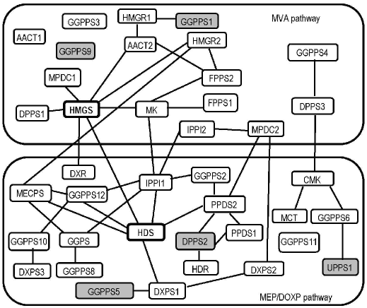
Figure 1: Biological network of the isoprenoid pathways inferred by using PLLM. Upper part: Genes of MVA pathway. Lower part: Genes of MEP/DOXP pathway. Grey boxes refer to mithochondrial genes; HMGS and HDS represent the hubs of the two modules.

VI Conclusions

In this paper, we present a comparative study of three different methods to infer networks of dependencies by estimates of partial correlation coefficients in the typical situation when $n<p$. In particular, we consider the Moore-Penrose pseudoinverse method (PINV), the residual correlation method (RCM) and a covariance-regularized method $(\ell_{2C})$. Firstly, we evaluate AUCs and timing performances on simulated datasets and we find that PINV presents some instability in AUC outcomes associated to the variable number variations. On the other hand, the two regularized methods show comparable performances with a sensible gain of time elapsing of $\ell_{2C}$ with respect to RCM. Finally, we present the results of an application of $\ell_{2C}$ for the inference of a gene network for isoprenoid pathways in A. thaliana. We find a negative partial correlation coefficient between HMGS and HDS, that are the two hubs in the two isoprenoid pathways. This means that they respond differently to the several tested experimental conditions and, together with the high connectivity of the two hubs, provides an evidence of cross-talk between genes in the plastidial and the cytosolic pathways. This evidence did not result from studies at level of single gene. Moreover, studies that infer this network by using only low-order partial correlation coefficients find more interactions between the two pathways with respect to the $\ell_{2C}$ method. A reduced number of edges between the two pathways is plausible considering the different cell compartmentalization of the two isoprenoid biosynthesis pathways.

- (1) Lauritzen, S.L.: Graphical models, Oxford University Press (1996)
- (2) Dempster, A.P.: Covariance Selection, Biometrics 28, 157–175 (1972)
- (3) H. Toh H., Horimoto., K.: System for automatically inferring a genetic network from expression profiles, J. Biol. Physics 28, 449–464 (2002)
- (4) Wille, A., Buhlmann, P.: Sparse graphical Gaussian modelling of the isoprenoid network in Arabidopsis thaliana, Genome Biology, 5, R92 (2004).
- (5) Castelo, R., Roverato, A.: A robust procedure for Gaussian graphical model search from microarray data with larger than , JMLR, 7, 2621–2650 (2006)
- (6) Gilbert, H.N., van der Laan, M.J, Dudoit, S.: Joint multiple testing procedures for graphical model selection with applications to biological networks, U.C. Berkeley Tech report, URL www.bepress.com/ucbbiostat/paper245 (2009).
- (7) Yuan, M., Lin, Y.: Model selection and estimation in the gaussian graphical model, Biometrika 94, 19–35 (2007)
- (8) Friedman, J., Hastie, T., Tibshirani R.: Sparse inverse covariance estimation with the graphical lasso, Biostatistics 9, 432–441 (2008)
- (9) Witten, D.M., Tibshirani, R.: Covariance-regularized regression and classifcation for high dimensional problems, J. R. Statist. Soc. B 71, 615-636 (2009)
- (10) Dobra, A., Hans, C., Jones, B., Nevins, J.R., West, M.: Sparse graphical models for exploring gene expression data, J. Multiv. Analysis 90, 196–212 (2004)
- (11) Schaffer, J., Strimmer, K.: An empirical Bayes approach to inferring large-scale gene association networks, Bioinformatics 21, 754–764 (2005)
- (12) Meinshausen N and P. Buhlmann 2006. High-dimensional graphs and variable selection with the lasso. Ann. Statist. 34, 1436–1462 (2006)
- (13) Friedman, J., Hastie, T., Tibshirani R.: Application of the lasso and grouped lasso to the estimation of sparse graphical models (2010)
- (14) Dikstra, R.L.: Establishing the positive definiteness of the sample covariance matrix, Ann. Math. Statist. 41, 2153–2154 (1970)
- (15) Girosi, F., Jones, M., Poggio, T.: Regularization Theory and Neural Networks Architectures, Neural Computation 7, 219–269 (1995)
- (16) Raudys,S., Duin, R.P.W.: Expected classification error of the Fisher linear classifier with pseudoinverse covariance matrix, Pattern Recogn. Lett. 19, 385–392 (1998)
- (17) Disch, A., Hemmerlin, A., Bach, T.J., Rohmer, M.: Mevalonate-derived isopentenyl diphosphate is the biosynthetic precursor of ubiquinone prenyl side chain in tobacco BY-2 cells, Biochem. J. 331, 615–621 (1998)
- (18) Lichtenthaler, H.K., Schwender, J., Disch, A., Rohmer, M.: Biosynthesis of isoprenoids in higher plant chloroplasts proceeds via a mevalonate-independent pathway, FEBS Lett. 400, 271–274 (1997)
- (19) Laule, O., F rholz, A., Chang, H.S., Zhu, T., Wang, X., Heifetz, P.B., Gruissem, W., Lange, M.: Crosstalk between cytosolic and plastidial pathways of isoprenoid biosynthesis in Arabidopsis thaliana, PNAS 100, 6866–6871 (2003)
- (20) Ihmels J, Levy R, Barkai N: Principles of transcriptional control in the metabolic network of Saccharomyces cerevisiae. Nat Biotechnol 22, 86–92 (2004).