Planar percolation with a glimpse of Schramm–Loewner Evolution

Abstract

In recent years, important progress has been made in the field of two-dimensional statistical physics. One of the most striking achievements is the proof of the Cardy–Smirnov formula. This theorem, together with the introduction of Schramm–Loewner Evolution and techniques developed over the years in percolation, allow precise descriptions of the critical and near-critical regimes of the model. This survey aims to describe the different steps leading to the proof that the infinite-cluster density $\theta(p)$ for site percolation on the triangular lattice behaves like $(p-p_{c})^{5/36+o(1)}$ as $p\searrow p_{c}=1/2$.

t1This is an original survey paper

1 Introduction

Percolation as a physical model was introduced by Broadbent and Hammersley in the fifties [BH57]. For $p\in(0,1)$, (site) percolation on the triangular lattice $\mathbb{T}$ is a random configuration supported on the vertices (or sites), each one being open with probability $p$ and closed otherwise, independently of the others. This can also be seen as a random coloring of the faces of the hexagonal lattice $\mathbb{H}$ dual to $\mathbb{T}$. Denote the measure on configurations by $\mathbb{P}_{p}$. For general background on percolation, we refer the reader to the books of Grimmett [Gri99] and Kesten [Kes82].

We will be interested in the connectivity properties of the model. Two sets of sites $A$ and $B$ of the triangular lattice are connected (which will be denoted by $A\leftrightarrow B$) if there exists an open path, i.e. a path of neighboring open sites, starting at $a\in A$ and ending at $b\in B$. If there exists a closed path, i.e. a path of neighboring closed sites, starting at $a\in A$ and ending at $b\in B$, we will write $A\stackrel{{\scriptstyle*}}{{\leftrightarrow}}B$. If $A=\{a\}$ and $B=\{b\}$, we simply write $a\leftrightarrow b$. We also write $a\leftrightarrow\infty$ if $a$ is on an infinite open simple path. A cluster is a connected component of open sites.

It is classical that there exists $p_{c}\in(0,1)$ such that for $p<p_{c}$, there exists almost surely no infinite cluster, while for $p>p_{c}$, there exists almost surely a unique such cluster. This parameter is called the critical point.

Theorem 1.1.

The critical point of site-percolation on the triangular lattice equals $1/2$.

A similar theorem was first proved in the case of bond percolation on the square lattice by Kesten in [Kes80].

Once the critical point has been determined, it is natural to study the phase transition of the model, i.e. its behavior for $p$ near $p_{c}$. Physicists are interested in the thermodynamical properties of the model, such as the infinite cluster density

$$\theta(p):=\mathbb{P}_{p}(0\leftrightarrow\infty)\text{ when $p>p_{c}$,}$$

the susceptibility (or mean cluster-size)

$$\chi(p):=\sum_{x\in\mathbb{T}}\mathbb{P}_{p}(0\leftrightarrow x)\text{ when $p<p_{c}$,}$$

and the correlation length $L_{p}$ (see Definition 4.5). The behavior of these quantities near $p_{c}$ is believed to be governed by power laws:

$$\begin{array}[]{r@{\;}c@{\;}ll}\theta(p)&=&(p-p_{c})^{\beta+o(1)}&\text{as }p\searrow p_{c},\\ \chi(p)&=&(p-p_{c})^{-\gamma+o(1)}&\text{as }p\nearrow p_{c},\\ L_{p}&=&(p-p_{c})^{-\nu+o(1)}&\text{as }p\nearrow p_{c}.\\ \end{array}$$

These critical exponents $\beta$, $\gamma$ and $\nu$ (and others) are not independent of each other but satisfy certain equations called scaling relations. Kesten’s scaling relations relate $\beta$, $\gamma$ and $\nu$ to the so-called monochromatic one-arm and polychromatic four-arm exponents at criticality. The important feature of these relations is that they relate quantities defined away from criticality to fractal properties of the critical regime. In other words, the behavior of percolation through its phase transition (as $p$ varies from slightly below to slightly above $p_{c}$) is intimately related to its behavior at $p_{c}$. The scaling relations enable mathematicians to focus on the critical phase. If the connectivity properties of the critical phase can be understood, then critical exponents for $\theta$, $\chi$, $L$ will follow.

We now turn to the study of planar percolation at $p=p_{c}$ and briefly recall the history of the subject. In the seminal papers [BPZ84a] and [BPZ84b], Belavin, Polyakov and Zamolodchikov postulated conformal invariance (under all conformal transformations of sub-regions) in the scaling limit of critical two-dimensional statistical mechanics models, of which percolation at $p_{c}$ is one. The renormalization group formalism suggests that the scaling limit of critical models is a fixed point for the renormalization transformation. The fixed point being unique, the scaling limit should be invariant under translation, rotation and scaling. Since it can be described by quantum local fields, it is natural to expect that the field describing the scaling limit of the critical regime is itself invariant under all transformations which are locally compositions of translations, rotations and scalings. These transformations are exactly the conformal maps.

From a mathematical perspective, the notion of conformal invariance of an entire model is ill-posed, since the meaning of scaling limit depends on the object we wish to study (interfaces, size of clusters, crossings, etc). A mathematical setting for studying scaling limits of interfaces has been developed, therefore we will focus on this aspect in this document.

Let us start with the study of a single curve. Fix a simply connected planar domain $(\Omega,a,b)$ with two points on the boundary and consider discretizations $(\Omega_{\delta},a_{\delta},b_{\delta})$ of $(\Omega,a,b)$ by a triangular lattice of mesh size $\delta$. The clockwise boundary arc of $\Omega_{\delta}$ from $a_{\delta}$ to $b_{\delta}$ is called $a_{\delta}b_{\delta}$, and the one from $b_{\delta}$ to $a_{\delta}$ is called $b_{\delta}a_{\delta}$. Assume now that the sites of $a_{\delta}b_{\delta}$ are open and that those of $b_{\delta}a_{\delta}$ are closed. There exists a unique interface consisting of bonds of the dual hexagonal lattice, between the open cluster of $a_{\delta}b_{\delta}$ and the closed cluster of $b_{\delta}a_{\delta}$ (in order to see this, the correspondence between face percolation on the hexagonal lattice and site percolation on the triangular one is useful). We call this interface the exploration path and denote it by $\gamma_{\delta}$; see the figure on the first page.

Conformal field theory leads to the prediction that $\gamma_{\delta}$ converges as $\delta\rightarrow 0$ to a random, continuous, non-self-crossing curve from $a$ to $b$ staying in $\Omega$, and which is expected to be conformally invariant in the following sense.

Definition 1.2.

A family of random non-self-crossing continuous curves $\gamma_{(\Omega,a,b)}$, going from $a$ to $b$ and contained in $\Omega$, indexed by simply connected domains with two marked points on the boundary $(\Omega,a,b)$ is conformally invariant if for any $(\Omega,a,b)$ and any conformal map $\psi:\Omega\rightarrow\mathbb{C}$,

$$\psi(\gamma_{(\Omega,a,b)})~{}\text{has the same law as}~{}\gamma_{(\psi(\Omega),\psi(a),\psi(b))}.$$

In 1999, Schramm proposed a natural candidate for such conformally invariant families of curves. He noticed that the interfaces of various models satisfy the domain Markov property (see Section 2.4) which, together with the assumption of conformal invariance, determines a one-parameter family of such curves. In [Sch00], he introduced the Stochastic Loewner evolution (${\mathrm{SLE}}$ for short) which is now known as the Schramm–Loewner evolution. For $\kappa>0$, a domain $\Omega$ and two points $a$ and $b$ on its boundary, ${\mathrm{SLE}}(\kappa)$ is the random Loewner evolution in $\Omega$ from $a$ to $b$ with driving process $\sqrt{\kappa}B_{t}$, where $(B_{t})$ is a standard Brownian motion. We refer to [Wer09b] for a formal definition of ${\mathrm{SLE}}$. By construction, this process is conformally invariant, random and fractal. The prediction of conformal field theory then translates into the following prediction for percolation: the limit of $(\gamma_{\delta})_{\delta>0}$ in $(\Omega,a,b)$ is ${\mathrm{SLE}}(6)$.

For completeness, let us mention that when considering not only a single curve but multiple interfaces, families of interfaces in a percolation model are also expected to converge in the scaling limit to a conformally invariant family of non-intersecting loops. Sheffield and Werner [SW10a, SW10b] introduced a one-parameter family of probability measures on collections of non-intersecting loops which are conformally invariant. These processes are called the Conformal Loop Ensembles ${\mathrm{CLE}}(\kappa)$ for $\kappa>8/3$. The ${\mathrm{CLE}}(\kappa)$ process is related to the ${\mathrm{SLE}}(\kappa)$ in the following manner: the loops of ${\mathrm{CLE}}(\kappa)$ are locally similar to ${\mathrm{SLE}}(\kappa)$.

Even though we now have a mathematical framework for conformal invariance, it remains an extremely hard task to prove convergence of the interfaces in $(\Omega_{\delta},a_{\delta},b_{\delta})$ to ${\mathrm{SLE}}$. Nevertheless, the observation that properties of interfaces should also be conformally invariant led Langlands, Poulliot and Saint-Aubin to publish in [LPSA94] numerical values in agreement with the conformal invariance in the scaling limit of crossing probabilities in the percolation model. More precisely, consider a Jordan domain $\Omega$ with four points $A,B,C$ and $D$ on the boundary. The $5$-tuple $(\Omega,A,B,C,D)$ is called a topological rectangle. The authors checked numerically that the probability $\mathcal{C}_{\delta}(\Omega,A,B,C,D)$ of having a path of adjacent open sites between the boundary arcs $AB$ and $CD$ converges as $\delta$ goes to $0$ towards a limit which is the same for $(\Omega,A,B,C,D)$ and $(\Omega^{\prime},A^{\prime},B^{\prime},C^{\prime},D^{\prime})$ if they are images of each other by a conformal map. Notice that the existence of such a crossing property can be expressed in terms of properties of a well-chosen interface, thus keeping this discussion in the frame proposed earlier.

The paper [LPSA94], while only numerical, attracted many mathematicians to the domain. The authors attribute the conjecture on conformal invariance of the limit of crossing probabilities to Aizenman. The same year, Cardy [Car92] proposed an explicit formula for the limit. In 2001, Smirnov proved Cardy’s formula rigorously for critical site percolation on the triangular lattice, hence rigorously providing a concrete example of a conformally invariant property of the model.

Theorem 1.3 (Smirnov [Smi01]).

For any topological rectangle $(\Omega,A,B,C,D)$, the probability of the event $\mathcal{C}_{\delta}(\Omega,A,B,C,D)$ has a limit $f(\Omega,A,B,C,D)$ as $\delta$ goes to $0$. Furthermore, the limit satisfies the following two properties:

• It is equal to $AB/AC$ if $\Omega$ is an equilateral triangle with vertices $A$, $C$ and $D$;

• It is conformally invariant, in the following sense: if $\,\Phi$ is a conformal map from $\Omega$ to another simply connected domain $\Phi(\Omega)$, which extends continuously to $\partial\Omega$, then

  $$f(\Omega,A,B,C,D)=f(\Phi(\Omega),\Phi(A),\Phi(B),\Phi(C),\Phi(D)).$$

The fact that Cardy’s formula takes such a simple form for equilateral triangles was first observed by Carleson. Notice that the Riemann mapping theorem along with the second property give the value of $f$ for every conformal rectangle.

A remarkable consequence of this theorem is that, even though Cardy’s formula provides information on crossing probabilities only, it can in fact be used to prove much more. We will see that it implies convergence of interfaces to the trace of ${\mathrm{SLE}}(6)$ (see Section 2.4). In other words, conformal invariance of one well-chosen quantity can be sufficient to prove conformal invariance of interfaces.

Theorem 1.4 (Smirnov, see also [CN07]).

Let $\Omega$ be a simply connected domain with two marked points $a$ and $b$ on the boundary. Let $\gamma_{\delta}$ be the exploration path of critical percolation as described in the previous paragraphs. Then the law of $\gamma_{\delta}$ converges weakly, as $\delta\rightarrow 0$, to the law of the trace of ${\mathrm{SLE}}(6)$ in $(\Omega,a,b)$.

Here and in later statements, the topology is associated to the distance on curves in $\Omega$ from $a$ to $b$ defined by

$$d(\Gamma,\tilde{\Gamma})=\inf_{\varphi}\sup_{t\geq 0}|\Gamma(t)-\tilde{\Gamma}(\varphi(t))|,$$

where the infimum is over all strictly increasing functions from $\mathbb{R}_{+}$ onto itself.

Similarly, one can consider the convergence of the whole family of discrete interfaces between open and closed clusters. This family converges to ${\mathrm{CLE}}(6)$, as was proved in [CN06], thus providing a proof of the full conformal invariance of percolation interfaces.

Convergence to ${\mathrm{SLE}}(6)$ is important for many reasons. Since ${\mathrm{SLE}}$ itself is very well understood (its fractal properties in particular), it enables the computation of several critical exponents describing the critical phase. We will introduce these exponents later in the survey. For now we state the result informally (see Theorem 3.4 or [SW01]):

• the probability that there exists an open path from the origin to the boundary of the box of radius $n$ behaves as $n^{-5/48+o(1)}$ as $n$ tends to infinity;

• the probability that there exist four arms, two open and two closed, from the origin to the boundary of the box of size $n$, behaves as $n^{-5/4+o(1)}$ as $n$ tends to infinity.

Together with Kesten’s scaling relations (Theorem 4.8 or [Kes87]), the previous asymptotics imply the following result, which is the main focus of this survey:

Theorem 1.5.

For site percolation on the triangular lattice, $p_{c}=1/2$ and

$$\theta(p)=(p-1/2)^{5/36+o(1)}\qquad\text{as $p\searrow 1/2$}.$$

Figure 1: Cluster density with respect to $p$. Non-trivial facts in this picture include $p_{c}=1/2$, $\theta(p_{c})=0$ and the behavior of $p\rightarrow\theta(p)$ near the critical point.

Organization of the survey

The next section is devoted to the geometry of percolation with $p=1/2$. First, we obtain uniform bounds for box crossing probabilities (via a RSW-type argument). Then, we prove the Cardy-Smirnov formula (Theorem 1.3). Finally, we sketch the proof of convergence to ${\mathrm{SLE}}(6)$ (Theorem 1.4).

The second section deals with critical exponents at criticality. We present the derivation of arm-exponents assuming some basic estimates on ${\mathrm{SLE}}$ processes.

The third section studies percolation away from $p=1/2$. We prove that $p_{c}=\frac{1}{2}$ and we introduce the notion of correlation length for general $p$. Then, we study the properties of percolation at scales smaller than the correlation length. Finally, we investigate Kesten’s scaling relations and prove Theorem 1.5.

The last section gathers a few open questions relevant to the topic.

Notation and standard correlation inequalities in percolation

Lattice, distance and balls

Except if otherwise stated, $\mathbb{T}$ will denote the triangular lattice with mesh size $1$, embedded in the complex plane ${\mathbb{C}}$, containing a vertex at the origin and a vertex at $1$. Complex coordinates will be used frequently to specify the location of a point. Let $d_{\mathbb{T}}(\cdot,\cdot)$ be the graph distance in $\mathbb{T}$. Define the ball $\Lambda_{n}:=\{x\in\mathbb{T}:d_{\mathbb{T}}(x,0)\leq n\}$ (balls have hexagonal shapes). Let $\partial\Lambda_{n}=\Lambda_{n}\setminus\Lambda_{n-1}$ be the internal boundary of $\Lambda_{n}$.

Increasing events

The Harris inequality and the monotonicity of percolation will be used a few times. We recall these two facts now. An event is called increasing if it is preserved by the addition of open sites, see Section 2.2 of [Gri99] (a typical example is the existence of an open path from one set to another). The inequality $p<p^{\prime}$ implies that $\mathbb{P}_{p}(A)\leq\mathbb{P}_{p^{\prime}}(A)$ for any increasing event $A$. Moreover, for every $p\in[0,1]$ and $A$, $B$ two increasing events,

$$\mathbb{P}_{p}(A\cap B)\geq\mathbb{P}_{p}(A)\mathbb{P}_{p}(B)\quad\quad\text{(Harris inequality)}.$$

The Harris inequality is a particular case of the Fortuin-Kasteleyn-Ginibre inequality [FKG71].

The van den Berg-Kesten inequality [vdBK85] will also be used extensively. For two increasing events $A$ and $B$, let $A\circ B$ be the event that $A$ and $B$ occur disjointly, meaning that $\omega\in A\circ B$ if and only if there exist a set of sites $E$ (possibly depending on $\omega$) such that any configuration $\omega^{\prime}$ with $\omega^{\prime}_{|E}=\omega_{|E}$ is in $A$ and any configuration $\omega^{\prime\prime}$ with $\omega^{\prime\prime}_{|\mathbb{T}\setminus E}=\omega_{|\mathbb{T}\setminus E}$ is in $B$. In words, the state of sites in $E$ is sufficient to verify whether $\omega$ is in $A$ or not, and similarly for $\mathbb{T}\setminus E$ for $B$. For instance, the event $\{a\leftrightarrow b\}\circ\{c\leftrightarrow d\}$, for $a,b,c,d$ four disjoint sites is the event that there exist two disjoint paths connecting $a$ to $b$ and $c$ to $d$ respectively. It is different from the event $\{a\leftrightarrow b\}\cap\{c\leftrightarrow d\}$ which requires only that there exist two paths connecting $a$ to $b$ and $c$ to $d$, but not necessarily disjoint.

For every $p\in[0,1]$ and $A$, $B$ two increasing events depending on a finite number of sites,

$$\mathbb{P}_{p}(A\circ B)\leq\mathbb{P}_{p}(A)\mathbb{P}_{p}(B)\quad\quad\text{(BK inequality)}.$$

This inequality was improved by Reimer [Rei00], who proved that the inequality is true for any two (non-necessarily increasing) events $A$ and $B$ depending on a finite number of sites.

References

For general background on percolation, we refer the reader to the books of Grimmett [Gri99], Bollobás and Riordan [BR06b] and Kesten [Kes82]. The proof of Cardy’s formula can be found in the original paper [Smi01]. Convergence of interfaces to ${\mathrm{SLE}}$ is proved in [CN07]. Scaling relations can be found in [Kes87, Nol08]. Lawler’s book [Law05] and Sun’s review [Sun11] are good places to get a general account on ${\mathrm{SLE}}$. We also refer to original research articles on the subject. More generally, subjects treated in this review are very close to those studied in Werner’s lecture notes [Wer09b].

2 Crossing probabilities and conformal invariance at the critical point

2.1 Circuits in annuli

In this whole section, we let $p=1/2$. Let $\mathcal{E}_{n}$ be the event that there exists a circuit (meaning a sequence of neighboring sites $x_{1},\dots,x_{n},x_{1}$) of open sites in $\Lambda_{3n}\setminus\Lambda_{n}$ that surrounds the origin.

Theorem 2.1.

There exists $C>0$ such that for every $n>0$, $\mathbb{P}_{\!\frac{1}{2}}(\mathcal{E}_{n})\geq C$.

This theorem was first proved in a corresponding form in the case of bond percolation on the square lattice by Russo [Rus78] and by Seymour and Welsh [SW78]. It has many applications, several of which will be discussed in this survey.

Such a bound (and its proof) is not surprising since open and closed sites play symmetric roles at $p=\frac{1}{2}$. It is natural to expect that the probability of $\mathcal{E}_{n}$ goes to $0$ (resp. $1$) for $p$ below (resp. above) $1/2$.

Proof.

We present one of the many proofs of Theorem 2.1, inspired by an argument due to Smirnov and presented in [Wer09a] (in French).

Step 1:

Let $n>0$ and index the sides of $\Lambda_{n}$ as in Fig. 2. Consider the event that $\ell_{1}$ is connected by an open path to $\ell_{3}\cup\ell_{4}$ in $\Lambda_{n}$. The triangular lattice being a triangulation, the complement of this event is that $\ell_{2}$ is connected by a closed path to $\ell_{5}\cup\ell_{6}$ in $\Lambda_{n}$. Using the symmetry between closed and open sites and the invariance of the model under rotations of angle $\pi/3$ around the origin, $\mathbb{P}_{\!\frac{1}{2}}(\ell_{1}\leftrightarrow\ell_{3}\cup\ell_{4}\text{ in }\Lambda_{n})$ is equal to $1/2$. Let us emphasize that we used that $\mathbb{T}$ is a triangulation invariant under rotations of angle $\pi/3$.

In fact, we also have that $\smash{\mathbb{P}_{\!\frac{1}{2}}}(\ell_{1}\leftrightarrow\ell_{4}\text{ in }\Lambda_{n})\geq 1/8$. Indeed, either this is true or, going to the complement, $\mathbb{P}_{\!\frac{1}{2}}(\ell_{1}\leftrightarrow\ell_{3}\text{ in }\Lambda_{n})\geq 1/2-1/8$. But in this case, using the Harris inequality,

$$\mathbb{P}_{\!\frac{1}{2}}(\ell_{1}\leftrightarrow\ell_{4}\text{ in }\Lambda_{n})\geq\mathbb{P}_{\!\frac{1}{2}}(\ell_{1}\leftrightarrow\ell_{3}\text{ in }\Lambda_{n})\mathbb{P}_{\!\frac{1}{2}}(\ell_{2}\leftrightarrow\ell_{4}\text{ in }\Lambda_{n})\geq(3/8)^{2}\geq 1/8.$$

Step 2:

Let $i=\sqrt{-1}$. Consider $R_{n}=\Lambda_{n}\cup(\Lambda_{n}-\sqrt{3}n{i})$ and index the sides of $R_{n}$ as in Fig. 2. For a path $\gamma$ from $\ell_{1}$ to $\ell_{4}$ in $\Lambda_{n}$, define the domain $\Omega_{\gamma}$ to consist of the sites of $R_{n}$ strictly to the right of $\gamma\cup\sigma(\gamma)$, where $\sigma$ is the reflection with respect to $\ell_{1}$. Once again, the complement of $\{\ell_{4}\cup\gamma\leftrightarrow\ell_{10}\cup\ell_{11}$ in $\Omega_{\gamma}\}$ is $\{\ell_{9}\cup\sigma(\gamma)\stackrel{{\scriptstyle*}}{{\leftrightarrow}}\ell_{2}\cup\ell_{3}$ in $\Omega_{\gamma}\}$. The switching of colors and the symmetry with respect to $\ell_{1}$ imply that the probability of the former is at least $1/2$ (it is not equal to $1/2$ since the site on $\ell_{1}$ is necessarily open).

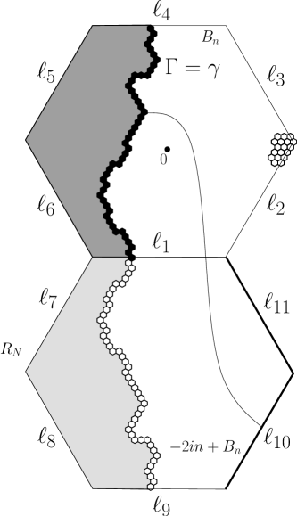
Figure 2: The dark gray area is the set of sites which are discovered after conditioning on $\{\Gamma=\gamma\}$. The white area is $\Omega_{\gamma}$.

If $E:=\{\ell_{1}\leftrightarrow\ell_{4}\text{ in $\Lambda_{n}$}\}$ occurs, set $\Gamma$ to be the left-most crossing between $\ell_{1}$ and $\ell_{4}$. For a given path $\gamma$ from $\ell_{1}$ to $\ell_{4}$, the event $\{\Gamma=\gamma\}$ is measurable only in terms of sites to the left or in $\gamma$. In particular, conditioning on $\{\Gamma=\gamma\}$, the configuration in $\Omega_{\gamma}$ is a percolation configuration. Thus,

$$\mathbb{P}_{\!\frac{1}{2}}\big{(}(\ell_{4}\cup\gamma)\leftrightarrow(\ell_{10}\cup\ell_{11})\text{ in }\Omega_{\gamma}~{}|~{}\Gamma=\gamma\big{)}~{}\geq~{}1/2.$$

Therefore,

$$\mathbb{P}_{\!\frac{1}{2}}\big{(}\ell_{4}\leftrightarrow(\ell_{10}\cup\ell_{11})\text{~{}in $R_{n}$}\big{)}~{} =~{}\mathbb{P}_{\!\frac{1}{2}}\big{(}\ell_{4}\leftrightarrow(\ell_{10}\cup\ell_{11})\text{~{}in $R_{n}$}~{},~{}E\big{)}$$

$$=~{}\sum_{\gamma}\mathbb{P}_{\!\frac{1}{2}}\big{(}\ell_{4}\leftrightarrow(\ell_{10}\cup\ell_{11})\text{~{}in $R_{n}$}~{},~{}\Gamma=\gamma\big{)}$$

$$\geq~{}\sum_{\gamma}\mathbb{P}_{\!\frac{1}{2}}\big{(}(\ell_{4}\cup\gamma)\leftrightarrow(\ell_{10}\cup\ell_{11})\text{~{}in~{}}\Omega_{\gamma}~{},~{}\Gamma=\gamma\big{)}$$

$$\geq~{}\sum_{\gamma}\frac{1}{2}\mathbb{P}_{\!\frac{1}{2}}(\Gamma=\gamma)~{}=~{}\frac{1}{2}\mathbb{P}_{\!\frac{1}{2}}(E)~{}\geq~{}\frac{1}{16}.$$

Figure 3: Six “rectangles” which, when crossed, ensure the existence of a circuit in the annulus.

Step 3:

Invoking the Harris inequality,

$$\mathbb{P}_{\!\frac{1}{2}}(\ell_{4}\leftrightarrow\ell_{9})~{}\geq~{}\mathbb{P}_{\!\frac{1}{2}}\big{(}\ell_{4}\leftrightarrow(\ell_{10}\cup\ell_{11})\big{)}\mathbb{P}_{\!\frac{1}{2}}\big{(}(\ell_{2}\cup\ell_{3})\leftrightarrow\ell_{9}\big{)}~{}\geq\frac{1}{16^{2}}.$$

Assuming that the six subdomains of the space (which correspond to translations and rotations of $R_{n}$) described in Fig. 3 are crossed (in the sense that there are open paths between opposite short edges), the result follows from a final use of the Harris inequality. ∎

The first corollary of Theorem 2.1 is the following lower bound on $p_{c}$. The result can also be proved without Theorem 2.1 using an elegant argument by Zhang which invokes the uniqueness of the infinite cluster when it exists (see Section 11 of [Gri99]).

Corollary 2.2 (Harris [Har60]).

For site percolation on the triangular lattice, $\theta(1/2)=0$. In particular, $p_{c}\geq 1/2$.

Proof.

Let us prove that when $p=1/2$, $0$ is almost surely not connected by a closed path to infinity (it is the same probability for an open path). Let $N>0$. We consider the $N$ concentric disjoint annuli $\Lambda_{3^{n+1}}\setminus\Lambda_{3^{n}}$, for $0\leq n<N$, and we use that the behavior in each annulus is independent of the behavior in the others. Formally, the origin being connected to $\partial\Lambda_{3^{N}}$ by a closed path implies that for every $n<N$, the complement, $\mathcal{E}^{c}_{3^{n}}$, of $\mathcal{E}_{3^{n}}$ occurs. Therefore,

$$\mathbb{P}_{\!\frac{1}{2}}(0\stackrel{{\scriptstyle*}}{{\leftrightarrow}}\partial\Lambda_{3^{N}})~{} \leq~{}\mathbb{P}_{\!\frac{1}{2}}\left(\bigcap_{n<N}\mathcal{E}^{c}_{3^{n}}\right)~{}=~{}\prod_{n<N}\mathbb{P}_{\!\frac{1}{2}}\left(\mathcal{E}^{c}_{3^{n}}\right)~{}\leq~{}(1-C)^{N},$$ (1)

where $C$ is the constant in Theorem 2.1. In the second inequality, the independence between percolation in different annuli is crucial. In particular, the left-hand term converges to $0$ as $N\rightarrow\infty$, so that $\theta(1/2)=0$. Hence, by the definition of $p_{c}$, $p_{c}\geq 1/2$. ∎

2.2 Discretization of domains and crossing probabilities

In general, we are interested in crossing probabilities for general shapes. Consider a topological rectangle $(\Omega,A,B,C,D)$, i.e. a simply connected domain $\Omega\neq\mathbb{C}$ delimited by a non-intersecting continuous curve and four distinct points $A$, $B$, $C$ and $D$ on its boundary, indexed in counter-clockwise order. The eager reader might want to check that the argument of this section still goes through without the assumption that the boundary is a simple curve, when $A$, $B$, $C$ and $D$ are prime ends of $\Omega$ — in fact, this extension is needed if one wants to prove convergence to ${\mathrm{SLE}}_{6}$, because the boundary of a stopped ${\mathrm{SLE}}$ will typically not be a simple curve.

For $\delta>0$, we will be interested in percolation on $\Omega_{\delta}:=\Omega\cap\delta\mathbb{T}$ given by vertices of $\delta\mathbb{T}$ in $\Omega$ and edges entirely included in $\Omega$. Note that the boundary of $\Omega_{\delta}$ can be seen as a self-avoiding curve $s$ on $\Omega_{\delta}^{*}$ (which is a subgraph of the hexagonal lattice). Once again, this may not be true if the domain is not smooth, but we choose not to discuss this matter here. The graph $\Omega_{\delta}$ should be seen as a discretization of $\Omega$ at scale $\delta$. Let $A_{\delta}$, $B_{\delta}$, $C_{\delta}$ and $D_{\delta}$ be the dual sites in $s$ that are closest to $A$, $B$, $C$ and $D$ respectively. They divide $s$ into four arcs denoted by $A_{\delta}B_{\delta}$, $B_{\delta}C_{\delta}$, etc.

In the percolation setting, let $\mathcal{C}_{\delta}(\Omega,A,B,C,D)$ be the event that there is a path of open sites in $\Omega_{\delta}$ between the intervals $A_{\delta}B_{\delta}$ and $C_{\delta}D_{\delta}$ of its boundary (more precisely connecting two sites of $\Omega_{\delta}$ adjacent to $A_{\delta}B_{\delta}$ and $C_{\delta}D_{\delta}$ respectively). We call such a path an open crossing, and the event a crossing event; accordingly we will say that the rectangle is crossed if there exists an open crossing.

With a slight abuse of notation, we will denote the percolation measure with $p=1/2$ on $\delta\mathbb{T}$ by $\mathbb{P}_{\!\frac{1}{2}}$ (even though the measure is the push-forward of $\mathbb{P}_{\!\frac{1}{2}}$ by the scaling $x\mapsto\delta x$). We first state a direct consequence of Theorem 2.1:

Corollary 2.3 (Rough bounds on crossing probabilities).

Let $(\Omega,A,B,C,D)$ be a topological rectangle. There exist $0<c_{1},c_{2}<1$ such that for every $\delta>0$,

$$c_{1}~{}\leq~{}\mathbb{P}_{\!\frac{1}{2}}\big{[}\mathcal{C}_{\delta}(\Omega,A,B,C,D)\big{]}~{}\leq~{}c_{2}.$$

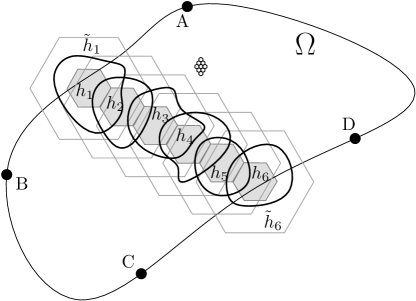
Figure 4: Circuits in annuli linking two arcs of a topological rectangle. If each of these annuli contains an open circuit disconnecting the interior from the exterior boundary, we obtain an open path connecting the two sides.

Proof.

It is sufficient to prove the lower bound, since the upper bound is a consequence of the following fact: the complement of $\mathcal{C}_{\delta}(\Omega,A,B,C,D)$ is the existence of a closed path from $B_{\delta}C_{\delta}$ to $D_{\delta}A_{\delta}$, it has same probability as $\mathcal{C}_{\delta}(\Omega,B,C,D,A)$. Therefore, if the latter probability is bounded from below, the probability of $\mathcal{C}_{\delta}(\Omega,A,B,C,D)$ is bounded away from $1$.

Fix $\varepsilon\in\delta\mathbb{N}$ positive. For a hexagon $h$ of radius $\varepsilon>0$, we set $\tilde{h}$ to be the hexagon with the same center and radius $3\varepsilon$. Now, consider a collection $h_{1}$, …, $h_{k}$ of hexagons “parallel” to the hexagonal lattice $\mathbb{H}$ (the dual lattice of $\mathbb{T}$) and of radius $\varepsilon$ satisfying the following conditions:

• $h_{1}$ intersects $AB$ and $h_{k}$ intersects $CD$,

• $\tilde{h}_{1}$, …, $\tilde{h}_{k}$ intersect neither $BC$ nor $DA$,

• $h_{i}$ are adjacent and the union of hexagons $h_{i}$ connects $AB$ to $CD$ in $\Omega$.

For any domain and any $\delta>0$ small enough, $\varepsilon>0$ can be chosen small enough so that the family $(h_{i})$ exists.

Let $E_{i}^{\delta}$ be the event that there is an open circuit in $\Omega_{\delta}\cap(\tilde{h}_{i}\setminus h_{i})$ surrounding $\Omega_{\delta}\cap h_{i}$. By construction, if each $E_{i}^{\delta}$ occurs, there is a path from $AB$ to $CD$, see Fig. 4. Using Theorem 2.1, the probability of this is bounded from below by $C^{k}$, where $C$ does not depend on $\varepsilon$ and $\delta$. Now, there exists a constant $K=K(\Omega)$ such that there is a choice of $\varepsilon>0$, $h_{1},\dots,h_{k}$, with $k\leq K$ working for any $\delta$ small enough, a fact which implies the claim. ∎

In particular, long rectangles are crossed in the long direction with probability bounded away from $0$ as $\delta\rightarrow 0$. This result is the classical formulation of Theorem 2.1. We finish this section with a property of percolation with parameter $1/2$:

Corollary 2.4.

There exist $\alpha,\beta>0$ such that for every $n>0$,

$$n^{-\alpha}~{}\leq~{}\mathbb{P}_{\!\frac{1}{2}}(0\leftrightarrow\partial\Lambda_{n})~{}\leq~{}n^{-\beta}.$$

Proof.

The existence of $\beta>0$ is proved as in (1). For the lower bound, we use the following construction. Define

$$R_{n}:=\big{\{}k\cdot 1+\ell\cdot e^{i\pi/3}:k\in[0,2^{n}]\text{ and }\ell\in[0,2^{n+1}]\big{\}}$$

if $n$ is odd, and

$$R_{n}:=\big{\{}k\cdot 1+\ell\cdot e^{i\pi/3}:k\in[0,2^{n+1}]\text{ and }\ell\in[0,2^{n}]\big{\}}$$

if it is even. Set $F_{n}$ to be the event that $R_{n}$ is crossed in the “long” direction. Corollary 2.3 implies the existence of $C_{1}>0$ such that $\mathbb{P}_{\!\frac{1}{2}}(F_{n})\geq C_{1}$ for every $n>0$. By the Harris inequality

$$\mathbb{P}_{\!\frac{1}{2}}(0\leftrightarrow\partial\Lambda_{3^{N}})~{}\geq\mathbb{P}_{\!\frac{1}{2}}\left(\bigcap_{n=0}^{N}F_{n}\right)~{}\geq~{}\prod_{n=0}^{N}\mathbb{P}_{\!\frac{1}{2}}(F_{n})~{}\geq~{}C_{1}^{N+1}.$$

This yields the existence of $\alpha>0$. ∎

2.3 The Cardy–Smirnov formula

The subject of this section is the proof of Theorem 1.3. The proof of this theorem is very well (and very shortly) exposed in the original paper [Smi01]. It has been rewritten in a number of places including [BR06c, Gri10, Wer09b]. We provide here a version of the proof which is mainly inspired by [Smi01] and [Bef07].

Proof.

Fix $(\Omega,A,B,C)$ a topological triangle and $z\in\Omega$ (with the same caveat as in the previous proof, we will silently assume the boundary of $\Omega$ to be smooth and simple, for notation’s sake, but the same argument applies to the general case of a simply connected domain). For $\delta>0$, $A_{\delta}$, $B_{\delta}$, $C_{\delta}$, $z_{\delta}$ are the closest points of $\Omega_{\delta}^{*}$ to $A$, $B$, $C$, $z$ respectively, as before. Define $E_{A,\delta}(z)$ to be the event that there exists a non-self-intersecting path of open sites in $\Omega_{\delta}$, separating $A_{\delta}$ and $z_{\delta}$ from $B_{\delta}$ and $C_{\delta}$. We define $E_{B,\delta}(z)$, $E_{C,\delta}(z)$ similarly, with obvious circular permutations of the letters. Let $H_{A,\delta}(z)$ (resp. $H_{B,\delta}(z)$, $H_{C,\delta}(z)$) be the probability of $E_{A,\delta}(z)$ (resp. $E_{B,\delta}(z)$, $E_{C,\delta}(z)$). The functions $H_{A,\delta}$, $H_{B,\delta}$ and $H_{C,\delta}$ are extended to piecewise linear functions on $\Omega$.

Figure 5: Picture of the event $E_{A,\delta}(z)$. Also depicted is one oriented edge $e$ with its associated dual edge $e^{*}$. The graph $\mathbb{T}_{\delta}$ is drawn with dotted lines while its dual $\mathbb{H}_{\delta}$ is drawn with solid lines.

The proof consists of three steps, the second one being the most important:

• Prove that $(H_{A,\delta},H_{B,\delta},H_{C,\delta})_{\delta>0}$ is a precompact family of functions (with variable $z$).

• Let $\tau=e^{2i\pi/3}$ and introduce the two sequences of functions defined by

  $$H_{\delta}(z) :=H_{A,\delta}(z)+\tau H_{B,\delta}(z)+\tau^{2}H_{C,\delta}(z),$$

  $$S_{\delta}(z) :=H_{A,\delta}(z)+H_{B,\delta}(z)+H_{C,\delta}(z).$$

  Show that any sub-sequential limits $h$ and $s$ of $(H_{\delta})_{\delta>0}$ and $(S_{\delta})_{\delta>0}$ are holomorphic. This statement is proved using Morera’s theorem, based on the study of discrete integrals.

• Use boundary conditions to identify the possible sub-sequential limits $h$ and $s$. This guarantees the existence of limits for $(H_{A,\delta},H_{B,\delta},H_{C,\delta})_{\delta>0}$. A byproduct of the proof is the exact computation of these limits.

Then, since $E_{C,\delta}(D_{\delta})$ is exactly the event $\mathcal{C}_{\delta}(\Omega,A,B,C,D)$, the limit of $H_{C,\delta}(D_{\delta})$ as $\delta$ goes to $0$ is also the limit of crossing probabilities.

Precompactness.

We only sketch this part of the proof. Let $K$ be a compact subset of $\Omega$. If two points $z,z^{\prime}\in K$ are surrounded by a common open (or closed) circuit, then the events $E_{A,\delta}(z^{\prime})$ and $E_{A,\delta}(z)$ are realized simultaneously. Hence, the difference $|H_{A,\delta}(z^{\prime})-H_{A,\delta}(z)|$ is bounded above by

$$\mathbb{P}_{\!\frac{1}{2}}[z_{\delta}\text{~{}and~{}}z^{\prime}_{\delta}\text{~{}are not surrounded by a common open or a closed circuit}].$$

Let $\eta>0$ be the distance between $K$ and $\Omega^{c}$. For $z$ and $z^{\prime}$, Theorem 2.1 can be applied in roughly $\log(|z-z^{\prime}|/\eta)/\log 3$ concentric annuli, hence there exist two positive constants $C_{K}$ and $\varepsilon_{K}$ depending only on $K$ such that, for every $\delta>0$,

$$\left|H_{A,\delta}(z^{\prime})-H_{A,\delta}(z)\right|\leqslant C_{K}\left|z^{\prime}-z\right|^{\varepsilon_{K}}$$ (2)

and a similar bound for $H_{B,\delta}$ and $H_{C,\delta}$. Furthermore, similar estimates can be obtained along the boundary of $\Omega$ as long as we are away from $A$, $B$ and $C$.

Since the functions are extended on the whole domain (see definition above), we obtain a family of uniformly Hölder maps from any compact subset of $\overline{\Omega}\setminus\{A,B,C\}$ to $[0,1]$. By the Arzelà-Ascoli theorem, the family is relatively compact with respect to uniform convergence. It is hence possible to extract a subsequence $(H_{A,\delta_{n}},H_{B,\delta_{n}},H_{C,\delta_{n}})_{n>0}$, with $\delta_{n}\to 0$, which converges uniformly on every compact to a triple of Hölder maps $(h_{A},h_{B},h_{C})$ from $\overline{\Omega}\setminus\{A,B,C\}$ to $[0,1]$. From now on, we set $h=h_{A}+\tau h_{B}+\tau^{2}h_{C}$ and $s=h_{A}+h_{B}+h_{C}$ (they are the limits of $(H_{\delta_{n}})_{n>0}$ and $(S_{\delta_{n}})_{n>0}$ respectively).

Holomorphicity of $h$ and $s$.

We treat the case of $h$; the case of $s$ follows the same lines. To prove that $h$ is holomorphic, one can apply Morera’s theorem (see e.g. [Lan99]). Formally, one needs to prove that the integral of $h$ along $\gamma$ is zero for any simple, closed, smooth curve $\gamma$ contained $\Omega$. In order to prove this statement, we show that $(H_{\delta_{n}})_{n}$ is a sequence of (almost) discrete holomorphic functions, where one needs to specify what is meant by discrete holomorphic. In our case, we take it to mean that discrete contour integrals vanish. We refer to [Smi10] for more details on discrete holomorphicity, including other definitions of it and its connections to statistical physics.

Consider a simple, closed, smooth curve $\gamma$ contained in $\Omega$. For every $\delta>0$, let $\gamma_{\delta}$ be a discretization of $\gamma$ contained in $\Omega_{\delta}$, i.e. a finite chain $(\gamma_{\delta}(k))_{0\leqslant k\leqslant N_{\delta}}$ of pairwise distinct sites of $\Omega_{\delta}$, ordered in the counter-clockwise direction, such that for every index $k$, $\gamma_{\delta}(k)$ and $\gamma_{\delta}(k+1)$ are nearest neighbors, and chosen in such a way that the Hausdorff distance between $\gamma_{\delta}$ and $\gamma$ goes to $0$ with $\delta$. Notice that $N_{\delta}$ can be taken of order $\delta^{-1}$, which we shall assume from now on.

For an edge $e\in\mathbb{H}_{\delta}$, define $e^{*}$ to be the rotation by $\pi/2$ of $e$ around its center (it is an edge of the triangular lattice). For an edge $e$ of the hexagonal lattice, let

$$H_{\delta}(e):=\frac{H_{\delta}(x)+H_{\delta}(y)}{2},$$

where $e=xy$ ($x$ and $y$ are the endpoints of the edge $e$).

An oriented edge $e^{*}$ of $\mathbb{T}_{\delta}$ belongs to $\gamma_{\delta}$ if it is of the form $\gamma_{\delta}(k)\gamma_{\delta}(k+1)$. In such a case, we set $e^{*}\in\gamma_{\delta}$. Define the discrete integral $I_{\gamma}^{\delta}(H)$ of $H_{\delta}$ (and similarly $I_{\gamma}^{\delta}(S)$ for $S_{\delta}$) along $\gamma_{\delta}$ by

$$I_{\gamma}^{\delta}(H):=\sum_{e^{*}\in\gamma}e^{*}H_{\delta}(e).$$

In the formula above, $e^{*}$ is considered as a vector in $\mathbb{C}$ of length $\delta$.

Our goal is now to prove that $I_{\gamma}^{\delta}(H)$ and $I_{\gamma}^{\delta}(S)$ converge to $0$ as $\delta$ goes to $0$. For every oriented edge $e=xy\in\mathbb{H}_{\delta}$, set

$$P_{A,\delta}(e)~{}=~{}\mathbb{P}_{\!\frac{1}{2}}\big{(}E_{A,\delta}(y)\setminus E_{A,\delta}(x)\big{)},$$

and similarly $P_{B,\delta}$ and $P_{C,\delta}$.

Lemma 2.5.

For any smooth $\gamma$, as $\delta$ goes to $0$,

$$I_{\gamma}^{\delta}(H) =\sum_{e^{*}\text{~{}surrounded by~{}}\gamma_{\delta}}e^{*}\left[P_{A,\delta}(e)+\tau P_{B,\delta}(e)+\tau^{2}P_{C,\delta}(e)\right]+o(1),$$ (3)

$$I_{\gamma}^{\delta}(S) =\sum_{e^{*}\text{~{}surrounded by~{}}\gamma_{\delta}}e^{*}\left[P_{A,\delta}(e)+P_{B,\delta}(e)+P_{C,\delta}(e)\right]+o(1),$$ (4)

where the sum runs over oriented edges of $\mathbb{T}_{\delta}$ surrounded by the closed curve $\gamma_{\delta}$.

Proof.

We treat the case of $H_{\delta}$; that of $S_{\delta}$ is similar. For every oriented edge $e=xy$ in $\mathbb{H}_{\delta}$, define

$$\partial_{e}H_{\delta}:=H_{\delta}(y)-H_{\delta}(x).$$

If $f$ is a face of $\mathbb{T}_{\delta}$, let $\partial f$ be its boundary oriented in counter-clockwise order, seen as a set of oriented edges. With these notations, we get the following identity:

$$I_{\gamma}^{\delta}(H)~{}=~{}\sum_{e^{*}\in\gamma_{\delta}}e^{*}H_{\delta}(e)~{}=~{}\sum_{f\text{~{}surrounded by~{}}\gamma_{\delta}}\sum_{e^{*}\in\partial f}e^{*}H_{\delta}(e),$$ (5)

where the first sum on the right is over all faces of $\mathbb{T}_{\delta}$ surrounded by the closed curve $\gamma_{\delta}$. Indeed, in the last equality, each boundary term is obtained exactly once with the correct sign, and each interior term appears twice with opposite signs. The sum of $e^{*}H_{\delta}(e)$ around $f$ can be rewritten in the following fashion:

$$\sum_{e^{*}\in\partial f}e^{*}H_{\delta}(e)=\sum_{e^{*}=uv\in\partial f}i\left(\frac{u+v}{2}-f\right)\partial_{e}H_{\delta},$$

where $f$ denotes the complex coordinate of the center of the face $f$. Putting this quantity in the sum (5), the term $\partial_{e}H_{\delta}=H_{\delta}(y)-H_{\delta}(x)$ appears twice for $x,y\in\mathbb{H}_{\delta}$ nearest neighbors bordered by two triangles in $\gamma_{\delta}$, and the factors $i(u+v)/2=i(x+y)/2$ cancel between the two occurrences (here $e^{*}=uv$), leaving only $i$ times the difference between the centers of the faces, i.e. the complex coordinate of the edge $e^{*}$. Therefore,

$$I_{\gamma}^{\delta}(H)=\frac{1}{2}\sum_{e^{*}\subset Int(\gamma_{\delta})}e^{*}\partial_{e}H_{\delta}+o(1).$$ (6)

In the previous equality, we used the fact that the total contribution of the boundary goes to $0$ with $\delta$. Indeed, $e^{*}$ is of order $\delta$, and

$$\partial_{e}H_{\delta}~{}=~{}P_{A,\delta}(e)-P_{A,\delta}(-e)~{}+~{}\tau(P_{B,\delta}(e)-P_{B,\delta}(-e))~{}+~{}\tau^{2}(P_{C,\delta}(e)-P_{C,\delta}(-e)),$$ (7)

so that Theorem 2.1 gives a bound of $\delta^{1+\varepsilon}$ for $e^{*}\partial_{e}H_{\delta}$ (one may for instance perform a computation similar to the one used for precompactness). Since there are roughly $\delta^{-1}$ boundary terms, we obtain that the boundary accounts for at most $\delta^{\varepsilon}$.

Replacing $\partial H_{\delta}$ by (7) in the equation (6), and re-indexing the sum to obtain each oriented edge in exactly one term, we get the announced equality (3). ∎

Lemma 2.6 (Smirnov [Smi01]).

For every three edges $e_{1},e_{2},e_{3}$ of $\Omega_{\delta}^{*}$ emanating from the same site, ordered counterclockwise, we have the following identities:

$$P_{A,\delta}(e_{1})=P_{B,\delta}(e_{2})=P_{C,\delta}(e_{3}).$$

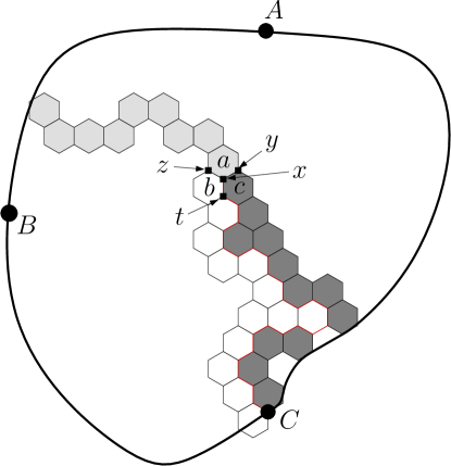
Figure 6: The dark gray and the white hexagons are the hexagons on $\overline{\Gamma}$, $\Gamma$ being in black.

Even though we include the proof for completeness, we refer the reader to [Smi01] for the (elementary, but very clever) first derivation of this result. The lemma extends to site-percolation with parameter $1/2$ on any planar triangulation.

Proof.

Index the three faces (of $\mathbb{H}_{\delta}$) around $x$ by $a$, $b$ and $c$, and the sites by $y$, $z$ and $t$ as depicted in Fig. 6.

Let us prove that $P_{A,\delta}(e_{1})=P_{B,\delta}(e_{2})$. The event $E_{A,\delta}(y)\setminus E_{A,\delta}(x)$ occurs if and only if there are open paths from $AB$ to $a$ and from $AC$ to $c$, and a closed path from $BC$ to $b$.

Consider the interface $\Gamma$ between the open clusters connected to $AC$ and the closed clusters connected to $BC$, starting at $C$, up to the first time it hits $x$ (it will do it if and only if there exist an open path from $AC$ to $c$ and a closed path from $BC$ to $b$). Fix a deterministic self-avoiding path of $\Omega^{*}_{\delta}$, denoted $\gamma$, from $C$ to $x$. The event $\{\Gamma=\gamma\}$ depends only on sites adjacent to $\gamma$ (we denote the set of such sites $\overline{\gamma}$). Now, on $\{\Gamma=\gamma\}$, there exists a bijection between configurations with an open path from $a$ to $AB$ and configurations with a closed path from $a$ to $AB$ (by symmetry between open and closed sites in the domain $\Omega_{\delta}\setminus\overline{\gamma}$). This is true for any $\gamma$ (the fact that the path is required to be self-avoiding is crucial here), hence there is a bijection between the event

$$E_{A,\delta}(y)\setminus E_{A,\delta}(x)=\bigcup_{\gamma}~{}\{\Gamma=\gamma\}\cap\{a\leftrightarrow AB\text{ in }\Omega_{\delta}\setminus\overline{\gamma}\}$$

and

$$E:=\bigcup_{\gamma}~{}\{\Gamma=\gamma\}\cap\{a\stackrel{{\scriptstyle*}}{{\leftrightarrow}}AB\text{ in }\Omega_{\delta}\setminus\overline{\gamma}\}.$$

Note that $E_{B,\delta}(z)\setminus E_{B,\delta}(x)$ is the image of $E$ after switching the states of all sites of $\mathbb{T}_{\delta}$ (or equivalently faces of $\mathbb{H}_{\delta}$). Hence, the two events are in one-to-one correspondence. Since $\mathbb{P}_{\!\frac{1}{2}}$ is uniform on the set of configurations,

$$P_{A,\delta}(e_{1})=\mathbb{P}_{\!\frac{1}{2}}(E_{B,\delta}(z)\setminus E_{B,\delta}(x))=\mathbb{P}_{\!\frac{1}{2}}(E)=P_{B,\delta}(e_{2}).$$

This argument is the key step of the lemma, and is sometimes called the color-switching trick. ∎

We are now in a position to prove that $I_{\gamma}^{\delta}(H)$ and $I_{\gamma}^{\delta}(S)$ converge to $0$. From Lemmas 2.5 and 2.6, we obtain by re-indexing the sum

$$I_{\gamma}^{\delta}(H)~{}=~{}\sum_{e^{*}\subset Int(\gamma_{\delta})}(e^{*}+\tau(\tau.e)^{*}+\tau^{2}(\tau^{2}.e)^{*})P_{A}(e)+o(1)=o(1),$$

since

$$e^{*}+\tau(\tau.e)^{*}+\tau^{2}(\tau^{2}.e)^{*}=0.$$ (8)

Similarly, for $s$:

$$I_{\gamma}^{\delta}(S)~{}=~{}\sum_{e^{*}\subset Int(\gamma_{\delta})}(e^{*}+(\tau.e)^{*}+(\tau^{2}.e)^{*})P_{A}(e)+o(1)=o(1).$$

Here, we have used

$$e^{*}+(\tau.e)^{*}+(\tau^{2}.e)^{*}=0.$$ (9)

This concludes the proof of the holomorphicity of $h$ and $s$.

Identification of $s$ and $h$.

Let us start with $s$. Since it is holomorphic and real-valued, it is constant. It is easy to see from the boundary conditions (near a corner for instance) that it is identically equal to 1. Now consider $h$. Since $h$ is holomorphic, it is enough to identify boundary conditions to specify it uniquely.

Let $z\in\Omega$. Since $h_{A}(z)+h_{B}(z)+h_{C}(z)=1$, $h(z)$ is a barycenter of $1$, $\tau$ and $\tau^{2}$ hence it is inside the triangle with vertices $1$, $\tau$ and $\tau^{2}$. Furthermore, if $z$ is on the boundary of $\Omega_{\delta}^{*}$, lying between $B$ and $C$, $h_{A}(z)=0$ (using Theorem 2.1), thus $h_{B}(z)+h_{C}(z)=1$ (since $s=1$). Hence, $h(z)$ lies on the interval $[\tau,\tau^{2}]$ of the complex plane. Besides, $h(B)=\tau$ and $h(C)=\tau^{2}$, so $h$ induces a continuous map from the boundary interval $[BC]$ of $\Omega$ onto $[\tau,\tau^{2}]$. By Theorem 2.1 yet again (more precisely Corollary 2.3), $h$ is one-to-one on this boundary interval (we leave it as an exercise). Similarly, $h$ induces a bijection between the boundary interval $[AB]$ (resp. $[CA]$) of $\Omega$ and the complex interval $[1,\tau]$ (resp. $[\tau^{2},1]$). Putting the pieces together we see that $h$ is a holomorphic map from $\Omega$ to the triangle with vertices $1$, $\tau$ and $\tau^{2}$, which extends continuously to $\bar{\Omega}$ and induces a continuous bijection between $\partial\Omega$ and the boundary of the triangle.

From standard results of complex analysis (“principle of corresponding boundaries”, cf. for instance Theorem 4.3 in [Lan99]), this implies that $h$ is actually a conformal map from $\Omega$ to the interior of the triangle. But we know that $h$ maps $A$ (resp. $B$, $C$) to $1$ (resp. $\tau$, $\tau^{2}$). This determines $h$ uniquely and concludes the proof of Theorem 1.3. ∎

As a corollary of the proof, we get a nice expression for $h_{A}$: if $\Phi_{\Omega,A,B,C}$ is the conformal map from $\Omega$ to the triangle mapping $A$, $B$ and $C$ as previously (which means of course that $\Phi_{\Omega,A,B,C}=h$) then

$$H_{A,\delta}(z)\to\frac{2\Re e(\Phi_{\Omega,A,B,C}(z))+1}{3}.$$

If $\Omega$ is the equilateral triangle itself, then $h$ is the identity map and we obtain Cardy’s formula in Carleson’s form: if $D\in[CA]$ then

$$f(\Omega,A,B,C,D)~{}=~{}\frac{|CD|}{|AB|}.$$

It is also to be noted that (8) actually characterizes the triangular lattice (and therefore its dual, the hexagonal one), which explains why this proof works only for this lattice.

2.4 Scaling limit of interfaces

We now show how Theorem 1.3 can be used to show Theorem 1.4. We start by recalling several properties of ${\mathrm{SLE}}$ processes.

2.4.1 A crash-course on Schramm–Loewner Evolutions

In this paragraph, several non-trivial concepts about Loewner chains are used and we refer to [Law05] and [Sun11] for details. We briefly recall several useful facts in the next paragraph. We do not aim for completeness (see [Law05, Wer04, Wer05] for details). We simply introduce notions needed in the next sections. Recall that a domain is a simply connected open set not equal to $\mathbb{C}$. We first explain how a curve between two points on the boundary of a domain can be encoded via a real function, called the driving process. We then explain how the procedure can be reversed. Finally, we describe the Schramm-Loewner Evolution.

From curves in domains to the driving process

Set $\mathbb{H}$ to be the upper half-plane. Fix a compact set $K\subset\overline{\mathbb{H}}$ such that $H=\mathbb{H}\setminus K$ is simply connected. Riemann’s mapping theorem guarantees the existence of a conformal map from $H$ onto $\mathbb{H}$. Moreover, there are a priori three real degrees of freedom in the choice of the conformal map, so that it is possible to fix its asymptotic behavior as $z$ goes to $\infty$. Let $g_{K}$ be the unique conformal map from $H$ onto $\mathbb{H}$ such that

$$g_{K}(z)~{}:=~{}z+\frac{C}{z}+O\left(\frac{1}{z^{2}}\right).$$

The proof of the existence of this map is not completely obvious and requires Schwarz’s reflection principle. The constant $C$ is called the $h$-capacity of $K$. It acts like a capacity: it is increasing in $K$ and the $h$-capacity of $\lambda K$ is $\lambda^{2}$ times the $h$-capacity of $K$.

There is a natural way to parametrize certain continuous non-self-crossing curves $\Gamma:\mathbb{R}_{+}\rightarrow\overline{\mathbb{H}}$ with $\Gamma(0)=0$ and with $\Gamma(s)$ going to $\infty$ when $s\rightarrow\infty$. For every $s$, let $H_{s}$ be the connected component of $\mathbb{H}\setminus\Gamma[0,s]$ containing $\infty$. We denote by $K_{s}$ the hull created by $\Gamma[0,s]$, i.e. the compact set $\overline{\mathbb{H}}\setminus H_{s}$. By construction, $K_{s}$ has a certain $h$-capacity $C_{s}$. The continuity of the curve guarantees that $C_{s}$ grows continuously, so that it is possible to parametrize the curve via a time-change $s(t)$ in such a way that $C_{s(t)}=2t$. This parametrization is called the $h$-capacity parametrization; we will assume it to be chosen, and reflect this by using the letter $t$ for the time parameter from now on. Note that in general, the previous operation is not a proper reparametrization, since any part of the curve “hidden from $\infty$” will not make the $h$-capacity grow, and thus will be mapped to the same point for the new curve; it might also be the case that $t$ does not go to infinity along the curve (e.g. if $\Gamma$ “crawls” along the boundary of the domain), but this is easily ruled out by crossing-type arguments when working with curves coming from percolation configurations.

The curve can be encoded via the family of conformal maps $g_{t}$ from $H_{t}$ to $\mathbb{H}$, in such a way that

$$g_{t}(z)~{}:=~{}z+\frac{2t}{z}+O\left(\frac{1}{z^{2}}\right).$$

Under mild conditions, the infinitesimal evolution of the family $(g_{t})$ implies the existence of a continuous real valued function $W_{t}$ such that for every $t$ and $z\in H_{t}$,

$$\partial_{t}g_{t}(z)~{}=~{}\frac{2}{g_{t}(z)-W_{t}}.$$ (10)

The function $W_{t}$ is called the driving function of $\Gamma$. The typical required hypothesis for $W$ to be well-defined is the following Local Growth Condition:

For any $t\geq 0$ and for any $\varepsilon>0$, there exists $\delta>0$ such that for any $0\leq s\leq t$, the diameter of $g_{s}(K_{s+\delta}\setminus K_{s})$ is smaller than $\varepsilon$.

This condition is always satisfied in the case of curves (in general, Loewner chains can be defined for families of growing hulls, see [Law05] for additional details).

From a driving function to curves

It is important to notice that the procedure of obtaining $W$ form $\gamma$ is reversible under mild assumptions on the driving function. We restrict our attention to the upper half-plane.

If a continuous function $(W_{t})_{t>0}$ is given, it is possible to reconstruct $H_{t}$ as the set of points $z$ for which the differential equation (10) with initial condition $z$ admits a solution defined on $[0,t]$. We then set $K_{t}=\overline{\mathbb{H}}\setminus H_{t}$. The family of hulls $(K_{t})_{t>0}$ is said to be the Loewner Evolution with driving function $(W_{t})_{t>0}$.

So far, we did not refer to any curve in this construction. If there exists a parametrized curve $(\Gamma_{t})_{t>0}$ such that for any $t>0$, $H_{t}$ is the connected component of $\mathbb{H}\setminus\Gamma[0,t]$ containing $\infty$, the Loewner chain $(K_{t})_{t>0}$ is said to be generated by a curve. Furthermore, $(\Gamma_{t})_{t>0}$ is called the trace of $(K_{t})_{t>0}$.

A general necessary and sufficient condition for a parametrized non-self-crossing curve in $(\Omega,a,b)$ to be the time-change of the trace of a Loewner chain is the following:

1. Its $h$-capacity is continuous;

2. Its $h$-capacity is strictly increasing;

3. The hull generated by the curve satisfies the Local Growth Condition.

The Schramm-Loewner Evolution

We are now in a position to define Schramm–Loewner Evolutions:

Definition 2.7 (${\mathrm{SLE}}$ in the upper half-plane).

The chordal Schramm–Loewner Evolution in $\mathbb{H}$ with parameter $\kappa>0$ is the (random) Loewner chain with driving process $W_{t}:=\sqrt{\kappa}B_{t}$, where $B_{t}$ is a standard Brownian motion.

Loewner chains in other domains are easily defined via conformal maps:

Definition 2.8 (${\mathrm{SLE}}$ in a general domain).

Fix a domain $\Omega$ with two points $a$ and $b$ on the boundary and assume it has a nice boundary (for instance a Jordan curve). The chordal Schramm–Loewner evolution with parameter $\kappa>0$ in $(\Omega,a,b)$ is the image of the Schramm–Loewner evolution in the upper half-plane by a conformal map from $(\mathbb{H},0,\infty)$ onto $(\Omega,a,b)$.

The scaling properties of Brownian motion ensure that the definition does not depend on the choice of the conformal map involved; equivalently, the definition is consistent in the case $\Omega=\mathbb{H}$. Defined as such, SLE is a random family of growing hulls, but it can be shown that the Loewner chain is generated by a curve (see [RS05] for $\kappa\neq 8$ and [LSW04] for $\kappa=8$).

Markov domain property and SLE

To conclude this section, let us justify the fact that SLE traces are natural scaling limits for interfaces of conformally invariant models. In order to explain this fact, we need the notion of domain Markov property for a family of random curves. Let $(\Gamma_{(\Omega,a,b)})$ be a family of random curves from $a$ to $b$ in $\Omega$, indexed by domains $(\Omega,a,b)$.

Definition 2.9 (Domain Markov property).

A family of random continuous curves $\Gamma_{(\Omega,a,b)}$ in simply connected domains is said to satisfy the domain Markov property if for every $(\Omega,a,b)$ and every $t>0$, the law of the curve $\Gamma_{(\Omega,a,b)}[t,\infty)$ conditionally on $\Gamma_{(\Omega,a,b)}[0,t]$ is the same as the law of $\Gamma_{(\Omega_{t},\Gamma_{t},b)}$, where $\Omega_{t}$ is the connected component of $\Omega\setminus\Gamma_{t}$ having $b$ on its boundary.

Discrete interfaces in many models of statistical physics naturally satisfy this property (which can be seen as a variant of the Dobrushin-Lanford-Ruelle conditions for Gibbs measures, [Geo88]), and therefore their scaling limits, provided that they exist, also should. Schramm proved the following result in [Sch00], which in some way justifies ${\mathrm{SLE}}$ processes as the only natural candidates for such scaling limits:

Theorem 2.10 (Schramm [Sch00]).

Every family of random curves $\Gamma_{(\Omega,a,b)}$ which

• is conformally invariant,

• satisfies the domain Markov property, and

• satisfies that $\Gamma_{(\mathbb{H},0,\infty)}$ is scale invariant,

is the trace of a chordal Schramm–Loewner evolution with parameter $\kappa\in[0,\infty)$.

Remark 2.11.

It is formally not necessary to assume scale invariance of the curve in the case of the upper-half plane, because it can be seen as a particular case of conformal invariance; we keep it nevertheless in the previous statement because it is potentially easier, while still informative, to prove.

2.4.2 Strategy of the proof of Theorem 1.4

In the following paragraphs, we fix a simply-connected domain $\Omega$ with two points $a$ and $b$ on its boundary. We consider percolation with parameter $p=1/2$ on a discretization $\Omega_{\delta}$ of $\Omega$ by the rescaled triangular lattice $\delta\mathbb{T}$. Let $a_{\delta}$ and $b_{\delta}$ be two boundary sites of $\Omega_{\delta}^{*}$ near $a$ and $b$ respectively. As explained in the introduction, the boundary of $\Omega_{\delta}$ can be divided into two arcs $a_{\delta}b_{\delta}$ and $b_{\delta}a_{\delta}$. Assuming that the first arc is composed of open sites, and the second of closed sites, we obtain a unique interface defined on $\Omega_{\delta}^{*}$ between the open cluster connected to $a_{\delta}b_{\delta}$, and the closed cluster connected to $b_{\delta}a_{\delta}$. This path is denoted by $\gamma_{\delta}$ and is called the exploration path.

The strategy to prove that $(\gamma_{\delta})$ converges to the trace of ${\mathrm{SLE}}(6)$ follows three steps:

• First, prove that the family $(\gamma_{\delta})$ of curves is tight.

• Then, show that any sub-sequential limit can be reparametrized in such a way that it becomes the trace of a Loewner evolution with a continuous driving process.

• Finally, show that the only possible driving process for the sub-sequential limits is $\sqrt{6}B_{t}$ where $B_{t}$ is a standard Brownian motion.

The main step is the third one. In order to identify Brownian motion as the only possible driving process for the curve, we find computable quantities expressed in terms of the limiting curve. In our case, these quantities will be the limits of certain crossing probabilities. The fact that these (explicit) functions are martingales implies martingale properties of the driving process. Lévy’s theorem (which states that a continuous real-valued process $X$ such that both $X_{t}$ and $X_{t}^{2}-6t$ are martingales is necessarily of the form $\sqrt{6}B_{t}$) then gives that the driving process must be $\sqrt{6}B_{t}$.

2.4.3 Tightness of interfaces

Recall that the convergence of random parametrized curves (say with time-parameter in $\mathbb{R}$) is in the sense of the weak topology inherited from the following distance on curves:

$$d(\Gamma,\tilde{\Gamma})~{}=~{}\inf_{\phi}\sup_{u\in\mathbb{R}}|\Gamma(u)-\tilde{\Gamma}(\phi(u))|,$$ (11)

where the infimum is taken over all reparametrizations (i.e. strictly increasing continuous functions $\phi\colon\mathbb{R}\rightarrow\mathbb{R}$ with $\phi(0)=0$ and $\phi$ tends to infinity as $t$ tends to infinity).

In this section, the following theorem is proved:

Theorem 2.12.

Fix a domain $(\Omega,a,b)$. The family $(\gamma_{\delta})_{\delta>0}$ of exploration paths for critical percolation in $(\Omega,a,b)$ is tight.

The question of tightness for curves in the plane has been studied in the milestone paper [AB99]. In this paper, it is proved that a sufficient condition for tightness is the absence, on every scale, of annuli crossed back and forth an arbitrary large number of times.

For $\delta>0$, let $\mu_{\delta}$ be the law of a random path $\Gamma_{\delta}$ on $\Omega_{\delta}$ from $a_{\delta}$ to $b_{\delta}$. For $x\in\Omega$ and $r<R$, let $\Lambda_{r}(x)=x+\Lambda_{r}$ and $S_{r,R}(x)=\Lambda_{R}(x)\setminus\Lambda_{r}(x)$ and define $\mathcal{A}_{k}(x;r,R)$ to be the event that there exist $k$ disjoint sub-paths of the curve $\Gamma_{\delta}$ crossing between the outer and inner boundaries of $S_{r,R}(x)$.

Theorem 2.13 (Aizenman-Burchard [AB99]).

Let $\Omega$ be a simply connected domain and let $a$ and $b$ be two marked points on its boundary. For $\delta>0$, let $\Gamma_{\delta}$ denote a random path on $\Omega_{\delta}$ from $a_{\delta}$ to $b_{\delta}$ with law $\mu_{\delta}$.

If there exist $k\in\mathbb{N}$, $C_{k}<\infty$ and $\Delta_{k}>2$ such that for all $\delta<r<R$ and $x\in\Omega$,

$$\mu_{\delta}(\mathcal{A}_{k}(x;r,R))\leq C_{k}\Big{(}\frac{r}{R}\Big{)}^{\Delta_{k}},$$

then the family of curves $(\Gamma_{\delta})$ is tight.

We now show how to exploit this theorem in order to prove Theorem 2.12. The main tool is Theorem 2.1.

Proof of Theorem 2.12.

Fix $x\in\Omega$, $\delta<r<R$ and recall that the lattice has mesh size $\delta$. Let $k$ be a positive integer to be fixed later. By the Reimer inequality (recall that the Reimer inequality is simply the BK inequality for non-increasing events),

$$\mathbb{P}_{p}\big{(}\mathcal{A}_{k}(x;r,3r)\big{)}\leq\left[\mathbb{P}_{p}\big{(}\mathcal{A}_{1}(x;r,3r)\big{)}\right]^{k}.$$

Using Theorem 2.1, $\mathbb{P}_{p}\big{(}\mathcal{A}_{1}(x;r,3r))\leq 1-\mathbb{P}_{p}(\mathcal{E}_{r/\delta})<1-C$, where $\mathcal{E}_{n}$ is the event that there exists a closed circuit surrounding the annulus in $\Lambda_{3n}\setminus\Lambda_{n}$. Let us fix $k$ large enough so that $(1-C)^{k}<1/27$. The annulus $S_{r,R}(x)$ can be decomposed into roughly $\ln_{3}(R/r)$ annuli of the form $S_{3^{\ell}r,3^{\ell+1}r}(x)$. For this value of $k$,

$$\mathbb{P}_{p}(\mathcal{A}_{k}(x;r,R))\leq C\left(\frac{r}{R}\right)^{3},$$ (12)

for some constant $C>0$. Hence, Theorem 2.13 implies that the family $(\gamma_{\delta})$ is tight. ∎

2.4.4 Sub-sequential limits are traces of Loewner chains

In the previous paragraph, exploration paths (and therefore their traces, since they coincide) were shown to be tight. Let us consider a sub-sequential limit. We would like to show that, properly reparametrized, the limiting curve is the trace of a Loewner chain.

Theorem 2.14.

Any sub-sequential limit of the family $(\gamma_{\delta})_{\delta>0}$ of exploration paths is almost surely the time-change of the trace of a Loewner chain.

The discrete curves $\gamma_{\delta}$ are random Loewner chains, but this does not imply that sub-sequential limits are. Indeed, not every continuous non-self-crossing curve can be reparametrized as the trace of a Loewner chain, especially when it is fractal-like and has many double points. We therefore need to provide an additional ingredient.

Condition C1 of the previous section is easily seen to be automatically satisfied by continuous curves. Similarly, Condition C3 follows from the two others when the curve is continuous, so that the only condition to check is Condition C2.

This condition can be understood as being the fact that the tip of the curve is visible from $b$ at every time. In other words, the family of hulls created by the curve is strictly increasing. This is the case if the curve does not enter long fjords created by its past at every scale, see Fig. 7.

         

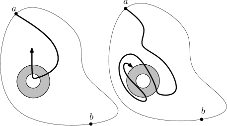
Figure 7: Left: An example of a fjord. Seen from $b$, the $h$-capacity (roughly speaking, the size) of the hull does not grow much while the curve is in the fjord. The event involves six alternating open (in plain lines) and closed (in dotted lines) crossings of the annulus. Right: Conditionally on the beginning of the curve, the crossing of the annulus is unforced on the left, while it is forced on the right.

Recently, Kemppainen and Smirnov proved a “structural theorem” characterizing sequences of random discrete curves whose limit satisfies Condition C2 almost surely. This theorem generalizes Theorem 2.13, in the sense that the condition is weaker and the conclusion stronger. Before stating the theorem, we need a definition. Fix $\Omega$ and two boundary points $a$ and $b$ and consider a curve $\Gamma$. A sub-path $\Gamma[t_{0},t_{1}]$ of a continuous curve $\Gamma$ is called a crossing of the annulus $S_{r,R}(x)$ if $\Gamma_{t_{0}}\in\partial\Lambda_{r}(x)$ and $\Gamma_{t_{1}}\in\partial\Lambda_{R}(x)$, where $t_{0}<t_{1}$ or $t_{1}<t_{0}$ and $\partial\Lambda_{r}$ is the boundary of $\Lambda_{r}$. A crossing is called unforced if there exists a path $\tilde{\Gamma}$ from $a$ to $b$ not intersecting $\Lambda_{R}(x)$.

Theorem 2.15 (Kemppainen-Smirnov, [KS10]).

Let $(\Omega,a,b)$ be a domain with two points on the boundary. For $\delta>0$, $\Gamma_{\delta}$ is a random continuous curve on $(\Omega_{\delta},a_{\delta},b_{\delta})$ with law $\mu_{\delta}$.

If there exist $C>1$ and $\Delta>0$ such that for any $0<\delta<r<R/C$ and for any stopping time $\tau$,

$$\mu_{\delta}(\gamma_{\delta}[\tau,\infty]\text{ contains an unforced crossing in $\Omega\setminus\gamma_{\delta}[0,\tau]$ of $S_{r,R}(x)$})\leq C\left(\frac{r}{R}\right)^{\Delta}$$

for any annulus $S_{r,R}(x)$, then the family $(\Gamma_{\delta})_{\delta>0}$ is tight and any sub-sequential limit can almost surely be reparametrized as the trace of a Loewner chain.

We do not prove this theorem and refer instead to the original article for a complete account. Theorem 2.1 implies the hypothesis of the previous theorem following the same lines as in the proof of Theorem 2.12. As a consequence, Theorem 2.14 follows readily.

In order to show Theorem 2.14 in the case of percolation, one can run an alternative argument based on Corollary 2.3 and the so-called 6-arm event. This argument has already been described precisely in [Wer09b]. For this reason, we do not repeat it here and refer to these lecture notes for details.

2.4.5 Convergence of exploration paths to ${\mathrm{SLE}}(6)$

Fix a topological triangle $(\Omega,A,B,C)$, i.e. a domain $\Omega\neq\mathbb{C}$ delimited by a non-intersecting continuous curve and three distinct points $A$, $B$ and $C$ on its boundary, indexed in counter-clockwise order. Let $(\Omega_{\delta},A_{\delta},B_{\delta},C_{\delta})$ be a discrete approximation of $(\Omega,A,B,C)$ and $z_{\delta}\in\Omega_{\delta}^{*}$. Recall the definition of $E_{A,\delta}(z_{\delta})$ used in the proof of Theorem 1.3: it is the event that there exists a non-self-intersecting path of open sites in $\Omega_{\delta}$, separating $A_{\delta}$ and $z_{\delta}$ from $B_{\delta}$ and $C_{\delta}$. For technical reasons, we keep the dependency on the domain in the notation for the duration of this section, and we set $E_{\Omega_{\delta},A_{\delta},B_{\delta},C_{\delta}}(z_{\delta}):=E_{A,\delta}(z_{\delta})$. Also define

$$H_{n}(\Omega_{\delta},A_{\delta},B_{\delta},C_{\delta},z_{\delta}):=\mathbb{P}_{\!\frac{1}{2}}(E_{\Omega_{\delta}\setminus\gamma[0,n],\gamma_{n},B_{\delta},C_{\delta}}(z_{\delta})).$$

Lemma 2.16.

For any $(\Omega,A,B,C)$, and for any $z\in\Omega$ and $\delta>0$, the function $(H_{n}(\Omega_{\delta},A_{\delta},B_{\delta},C_{\delta},z_{\delta}))_{n\geq 0}$ is a martingale with respect to $(\mathcal{F}_{n})_{n\geq 0}$, where $\mathcal{F}_{n}$ is the $\sigma$-algebra generated by the the first $n$ steps of $\gamma_{\delta}$.

Proof.

The slit domain created by “removing” the first $n$ steps of the exploration path is again a topological triangle. Conditionally on the $n$ first steps of $\gamma_{\delta}$, the law of the configuration in the new domain is exactly percolation in $\Omega\setminus\gamma_{\delta}[0,n]$. This observation implies that $H_{n}(\Omega_{\delta},A_{\delta},B_{\delta},C_{\delta},z_{\delta})$ is the random variable $1_{E_{\Omega_{\delta},A_{\delta},B_{\delta},C_{\delta}}(z_{\delta})}$ conditionally on $\mathcal{F}_{n}$, therefore it is automatically a martingale. ∎

Proposition 2.17.

Any sub-sequential limit of $(\gamma_{\delta})_{\delta>0}$ which is the trace of a Loewner chain is the trace of ${\mathrm{SLE}}(6)$.

Proof.

Once again, we only sketch the proof in order to highlight the important steps. Consider a sub-sequential limit $\gamma$ in the domain $(\Omega,A,B)$ which is a Loewner chain. Let $\phi$ be a map from $(\Omega,A,B)$ to $(\mathbb{H},0,\infty)$. Our goal is to prove that $\tilde{\gamma}:=\phi(\gamma)$ is a chordal ${\mathrm{SLE}}(6)$ in the upper half-plane.

Since $\gamma$ is assumed to be a Loewner chain, $\tilde{\gamma}$ is a growing hull from $0$ to $\infty$; we can assume that it is parametrized by its $h$-capacity. Let $W_{t}$ be its continuous driving process. Also define $g_{t}$ to be the conformal map from $\mathbb{H}\setminus\tilde{\gamma}[0,t]$ to $\mathbb{H}$ such that $g_{t}(z)=z+2t/z+O(1/z^{2})$ when $z$ goes to infinity.

Fix $C\in\partial\Omega$ and $Z\in\Omega$. For $\delta>0$, recall that $H_{n}(\Omega_{\delta},A_{\delta},B_{\delta},C_{\delta},Z_{\delta})$ is a martingale for $\gamma_{\delta}$. Since the martingale is bounded, $H_{\tau_{t}}(\Omega_{\delta},A_{\delta},B_{\delta},C_{\delta},Z_{\delta})$ is a martingale with respect to $\mathcal{F}_{\tau_{t}}$, where $\tau_{t}$ is the first time at which $\phi(\gamma_{\delta})$ has a $h$-capacity larger than $t$. Since the convergence of $\gamma_{\delta}$ to $\gamma$ is uniform on every compact subset of $(\Omega,A,B)$, one can see (with a little bit of work) that

$$H_{t}(Z):=\lim_{\delta\rightarrow 0}H_{\tau_{t}}(\Omega_{\delta},A_{\delta},B_{\delta},C_{\delta},Z_{\delta})$$

is a martingale with respect to $\mathcal{G}_{t}$, where $\mathcal{G}_{t}$ is the $\sigma$-algebra generated by the curve $\tilde{\gamma}$ up to the first time its $h$-capacity exceeds $t$. By definition, this time is $t$, and $\mathcal{G}_{t}$ is the $\sigma$-algebra generated by $\tilde{\gamma}[0,t]$. In other words, it is the natural filtration associated with the driving process $(W_{t})$.

We borrow the definitions of $h_{A}$ and $h$ from the proof of the Cardy–Smirnov formula. By first mapping $\Omega$ to $\mathbb{H}$ and then applying the Cardy-Smirnov formula, we find

$$H_{t}(Z)=h_{A}\left(\frac{g_{t}(z)-W_{t}}{g_{t}(c)-W_{t}}\right),$$

where we define $z:=\phi(Z)$ and $c:=\phi(C)$. This is a martingale for every choice of $z$ and $c$, so we get the family of identities

$$\mathbb{E}\left[h_{A}\left(\frac{g_{t}(z)-W_{t}}{g_{t}(c)-W_{t}}\right)\middle|\mathcal{G}_{s}\right]=h_{A}\left(\frac{g_{s}(z)-W_{s}}{g_{s}(c)-W_{s}}\right)$$

for all $z\in\mathbb{H}$, $c\in\mathbb{R}$ and $0<s<t$ such that $z$ and $c$ are both within the domain of definition of $g_{t}$. Now, we would like to express the previous equality in terms of $h$ instead of $h_{A}$ (recall that $h_{A}=\frac{1}{3}(2\Re e(h)+1)$). Noting that the two functions below, as functions of $z$, are holomorphic and equal at $c$, we obtain

$$\mathbb{E}\left[h\left(\frac{g_{t}(z)-W_{t}}{g_{t}(c)-W_{t}}\right)\middle|\mathcal{G}_{s}\right]=h\left(\frac{g_{s}(z)-W_{s}}{g_{s}(c)-W_{s}}\right).$$

We know the asymptotic expansion of $g_{s}$ and $g_{t}$ around infinity, so the above becomes

$$\mathbb{E}\left[h\left(\frac{z-W_{t}+2t/z+O(1/c^{2})}{c-W_{t}+2t/c+O(1/z^{2})}\right)\middle|\mathcal{G}_{s}\right]=h\left(\frac{z-W_{s}+2s/z+O(1/z^{2})}{c-W_{s}+2s/c+O(1/c^{2})}\right).$$ (13)

Letting $z$ and $c$ go to infinity with fixed ratio $z/c=\lambda\in\mathbb{H}$, we have

$$h\left(\frac{z-W_{s}+2s/z+O(1/z^{2})}{c-W_{s}+2s/c+O(1/c^{2})}\right) =h\left(\frac{\lambda-W_{s}/c+2s/\lambda c^{2}+O(1/c^{2})}{1-W_{s}/c+2s/c^{2}+O(1/c^{3})}\right)$$

$$=h\left(\lambda+\frac{(\lambda-1)W_{s}}{c}+\frac{(\lambda-1)W_{s}^{2}+2(1-\lambda^{2})s/\lambda}{c^{2}}+O(c^{-3})\right).$$

$$=h(\lambda)+\frac{(\lambda-1)h^{\prime}(\lambda)W_{s}}{c}$$

$$+\frac{(\lambda-1)W_{s}^{2}[h^{\prime}(\lambda)+(\lambda-1)h^{\prime\prime}(\lambda)/2]+2(1-\lambda^{2})sh^{\prime}(\lambda)/\lambda}{c^{2}}+O(c^{-3}).$$

Using this expansion on both sides of (13) and matching the terms, we obtain two identities for $(W_{t})$:

$$\mathbb{E}[W_{t}|\mathcal{G}_{s}]=W_{s},\quad E[W_{t}^{2}|\mathcal{G}_{s}]=W_{s}^{2}+\frac{4(1+\lambda)h^{\prime}(\lambda)/\lambda}{2h^{\prime}(\lambda)+(\lambda-1)h^{\prime\prime}(\lambda)}(t-s).$$

The function $h$ is a conformal map from the upper-half plane to the equilateral triangle, sending $0$, $1$ and $\infty$ to the vertices of the triangle; up to (explicit) additive and multiplicative constants $A$ and $B$, it can be written using the Schwarz-Christoffel formula as

$$h(\lambda)=A\int^{\lambda}[z(1-z)]^{-2/3}\;{\mathrm{d}}z+B.$$

From this, one obtains $h^{\prime}(\lambda)=A[\lambda(1-\lambda)]^{-2/3}$ and

$$\frac{h^{\prime\prime}(\lambda)}{h^{\prime}(\lambda)}=-\frac{2}{3}\left(\frac{1}{\lambda}-\frac{1}{1-\lambda}\right)=\frac{2(2\lambda-1)}{3\lambda(1-\lambda)}.$$

Plugging this into the previous expression shows that the coefficient of $(t-s)$ is identically equal to 6, and since we know that $(W_{t})$ is a continuous process, Lévy’s theorem implies that it is of the form $(\sqrt{6}B_{t})$ where $(B_{t})$ is a standard real-valued Brownian motion. This implies that $\gamma$ is the trace of the ${\mathrm{SLE}}(6)$ process in $(\Omega,A,B)$. ∎

Proof of Theorem 1.4.

By Theorem 2.12, the family of exploration processes is tight. Using Theorem 2.14, any sub-sequential limit is the time-change of the trace of a Loewner chain. Consider such a sub-sequential limit and parametrize it by its $h$-capacity. Proposition 2.17 then implies that it is the trace of SLE(6). The possible limit being unique, we are done. ∎

3 Critical exponents

To quantify connectivity properties at $p=1/2$, we introduce the notion of arm-event. Fix a sequence $\sigma\in\{0,1\}^{j}$ of $j$ colors (open $1$ or closed $0$). For $1\leq n<N$, define $A_{\sigma}(n,N)$ to be the event that there are $j$ disjoint paths from $\partial\Lambda_{n}$ to $\partial\Lambda_{N}$ with colors $\sigma_{1}$, …, $\sigma_{j}$ where the paths are indexed in counter-clockwise order. We set $A_{\sigma}(N)$ to be $A_{\sigma}(k,N)$ where $k$ is the smallest integer such that the event is non-empty. For instance, $A_{1}(n,N)$ is the one-arm event corresponding to the existence of an open crossing from the inner to the outer boundary of $\Lambda_{N}\setminus\Lambda_{n}$.

An adaptation of Corollary 2.4 implies that there exist $\alpha^{\prime}_{\sigma}$ and $\beta^{\prime}_{\sigma}$ such that

$$(n/N)^{\alpha^{\prime}_{\sigma}}~{}\leq~{}\mathbb{P}_{\!\frac{1}{2}}[A_{\sigma}(n,N)]~{}\leq~{}(n/N)^{\beta^{\prime}_{\sigma}}.$$

It is therefore natural to predict that there exists a critical exponent $\alpha_{\sigma}\in(0,\infty)$ such that

$$\mathbb{P}_{\!\frac{1}{2}}[A_{\sigma}(n,N)]~{}=~{}(n/N)^{\alpha_{\sigma}+o(1)},$$

where $o(1)$ is a quantity converging to 0 as $n/N$ goes to 0. The quantity $\alpha_{\sigma}$ is called an arm-exponent. We now explain how these exponents can be computed.

3.1 Quasi-multiplicativity of the probabilities of arm-events

Let us start by a few technical yet crucial statements on probabilities of arm-events. These statements will be instrumental in all the following proofs.

Theorem 3.1 (Quasi-multiplicativity).

Fix a color sequence $\sigma$. There exists $c\in(0,\infty)$ such that

$$c\mathbb{P}_{\!\frac{1}{2}}\big{[}A_{\sigma}(n_{1},n_{2})\big{]}\mathbb{P}_{\!\frac{1}{2}}\big{[}A_{\sigma}(n_{2},n_{3})\big{]}\leq\mathbb{P}_{\!\frac{1}{2}}\big{[}A_{\sigma}(n_{1},n_{3})\big{]}\leq\mathbb{P}_{\!\frac{1}{2}}\big{[}A_{\sigma}(n_{1},n_{2})\big{]}\mathbb{P}_{\!\frac{1}{2}}\big{[}A_{\sigma}(n_{2},n_{3})\big{]}$$

for every $n_{1}<n_{2}<n_{3}$.

The inequality

$$\mathbb{P}_{\!\frac{1}{2}}\big{[}A_{\sigma}(n_{1},n_{3})\big{]}\leq\mathbb{P}_{\!\frac{1}{2}}\big{[}A_{\sigma}(n_{1},n_{2})\big{]}\mathbb{P}_{\!\frac{1}{2}}\big{[}A_{\sigma}(n_{2},n_{3})\big{]}.$$

is straightforward using independence. The other one is slightly more technical. Let us mention that in the case of one arm ($\sigma=1$), or more generally if all the arms are to be of the same color, the proof is fairly easy (we recommend it as an exercise; see Fig. 8 for a hint). For general $\sigma$, the proof requires the notion of well-separated arms. We do not discuss this matter here and refer to the well-documented literature [Kes87, Nol08].

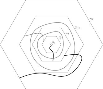
Figure 8: The paths in the annuli $\Lambda_{n_{3}}\setminus\Lambda_{n_{2}}$ and $\Lambda_{n_{2}}\setminus\Lambda_{n_{1}}$ are in black. A combination of two circuits connected by a path (in gray) connects the paths together. The combination of gray paths in the middle occurs with probability bounded away from 0 thanks to crossing estimates (Theorem 2.1 and Corollary 2.3).

Another important tool, which is also a consequence of the well-separation of arms, is the following localization of arms. Let $\delta>0$; for a sequence $\sigma$ of length $j$, consider $2j+1$ points $x_{1},x_{2},\dots,x_{2j},x_{2j+1}=x_{1}$ found in clockwise order on the boundary of $\Lambda_{n}$, with the additional condition that $|x_{k+1}-x_{k}|\geq\delta n$ for any $k\leq 2j$. Similarly, consider $2j+1$ points $y_{1},\dots,y_{2j},y_{2j+1}=y_{1}$ found in clockwise order on the boundary of $\Lambda_{N}$, with the additional condition that $|y_{k+1}-y_{k}|\geq\delta N$ for any $k\leq 2j$. The sequence of intervals $(I_{k}=[x_{2k-1},x_{2k}])_{k\leq j}$ and $(J_{k}=[y_{2k-1},y_{2k}])_{k\leq j}$ are called $\delta$-well separated landing sequences. Let $A^{I,J}_{\sigma}(n,N)$ be the event that for each $k$ there exists an arm of color $\sigma_{k}$ from $I_{k}$ to $J_{k}$ in $\Lambda_{n}\setminus\Lambda_{N}$, these arms being pairwise disjoint. This event corresponds to the event $A_{\sigma}(n,N)$ where arms are forced to start and finish in some prescribed areas of the boundary.

Proposition 3.2.

Let $\sigma$ be a sequence of colors; for any $\delta>0$ there exists $C_{\sigma}<\infty$ such that, for any $2n\leq N$ and any choice of $\delta$-well separated landing sequences $I,J$ at radii $n$ and $N$,

$$\mathbb{P}_{\!\frac{1}{2}}\big{[}A^{I,J}_{\sigma}(n,N)\big{]}\leq\mathbb{P}_{\!\frac{1}{2}}\big{[}A_{\sigma}(n,N)\big{]}\leq C_{\sigma}\mathbb{P}_{\!\frac{1}{2}}\big{[}A^{I,J}_{\sigma}(n,N)\big{]}.$$

Once again, only the second inequality is non trivial. We refer to [Nol08] for a comprehensive study.

3.2 Universal arm exponents

Before dealing with the computation of arm-exponents using SLE techniques, let us mention that several exponents can be computed without this elaborated machinery. These exponents, called universal exponents, are expected to be the same for a large class of models, including the so-called random-cluster models with cluster weights $q\leq 4$ (see [Gri06] for a review on the random-cluster model). In order to state the result, we need to define arm events in the half-plane. Let $\mathbb{H}^{+}$ be the set of vertices in $\mathbb{H}$ with positive second coordinate. For a color sequence $\sigma$ of $j$ colors, define $A_{\sigma}^{+}(n,N)$ to be the existence of $j$ disjoint paths in $(\Lambda_{N}\setminus\Lambda_{n})\cap\mathbb{H}^{+}$ from $\partial\Lambda_{n}\cap\mathbb{H}^{+}$ to $\partial\Lambda_{N}\cap\mathbb{H}^{+}$, colored counterclockwise according to $\sigma$.

Theorem 3.3.

For every $0<n<N$, there exist two constants $c,C\in(0,\infty)$ such that

$$c\left(\frac{n}{N}\right)^{2}\leq\mathbb{P}_{\!\frac{1}{2}}\big{[}A_{01001}(n,N)\big{]}\leq C\left(\frac{n}{N}\right)^{2},$$

$$c\left(\frac{n}{N}\right)^{2}\leq\mathbb{P}_{\!\frac{1}{2}}\big{[}A_{010}^{+}(n,N)\big{]}\leq C\left(\frac{n}{N}\right)^{2},$$

$$c\frac{n}{N}~{}\leq~{}\mathbb{P}_{\!\frac{1}{2}}\big{[}A_{01}^{+}(n,N)\big{]}~{}\leq~{}C\frac{n}{N}.$$

The three computations are based on the same type of ingredient, and we refer to [Wer09b] for a complete derivation. An important observation is that the proof of the above is based only on Theorem 3.1, Proposition 3.2 and crossing estimates (Corollary 2.3). It does not require conformal invariance.

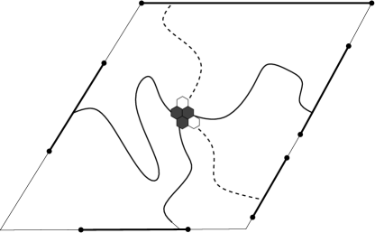
Figure 9: The landing sequences used to prove an upper bound on the probability of the 5-arm event. At most one site with five such arms exists.

Proof.

We only give a sketch of the proof of the first statement; the others are derived from similar arguments.

Consider percolation in a large $N\times N$ rectangle $R$, and mark five boundary intervals according to Fig. 9. It is easy to check that there is at most one site in the rectangle which is connected to these boundary arcs by disjoint arms of the depicted colors; in other words, the expected number of such hexagons is at most $1$. On the other hand, by arm localization, the probability for each of the hexagons in the middle $(N/3)\times(N/3)$ rectangle $R^{\prime}$ to exhibit $5$ such arms is given up to multiplicative constants by the probability of $5$ arms between radii $1$ and $N$, leading to the upper bound

$$\mathbb{P}_{\!\frac{1}{2}}\big{[}A_{01001}(1,N)\big{]}\leq C\left(\frac{1}{N}\right)^{2}.$$

To get the corresponding lower bound, we need to show that such a hexagon can be found with positive probability within $R^{\prime}$, and this in turn is a consequence of crossing estimates (Corollary 2.3). One way to proceed is as follows. Let $\Gamma$ be the highest horizontal, open crossing of $R$, provided such a crossing exists (which occurs with positive probability by Corollary 2.3). $\Gamma$ goes through $R^{\prime}$ with positive probability, and by definition, any hexagon on $\Gamma$ is connected to the top side of $R$ by a closed path. On the other hand, with positive probability, $\Gamma$ itself is connected to the bottom side of $R$ by an open path; let $\Gamma^{\prime}$ be the right-most such path, and let $X$ be the hexagon at which $\Gamma$ and $\Gamma^{\prime}$ intersect. Still with positive probability from Corollary 2.3, $X\in R^{\prime}$; and the absence of an open path further to the right imposes the existence of a closed path below $\Gamma$, connecting a neighbor of $X$ to the right-hand edge of $R$. Collecting all the information given by the construction, we see that from $X$ start five macroscopic disjoint arms of the same colors as in Fig. 9, from which the lower bound follows:

$$c\left(\frac{1}{N}\right)^{2}\leq\mathbb{P}_{\!\frac{1}{2}}\big{[}A_{01001}(1,N)\big{]}.$$

Similar bounds for $\mathbb{P}_{\!\frac{1}{2}}\big{[}A_{01001}(n,N)\big{]}$ may then be obtained invoking quasi-multiplicativity (Theorem 3.1), thus ending the argument. ∎

With the Reimer inequality (see the introduction), the first inequalities in the previous result imply several interesting inequalities on arm-exponents. For instance,

$$\mathbb{P}_{p}\big{[}A_{\sigma 1}(n,N)\big{]}\leq\mathbb{P}_{p}\big{[}A_{\sigma}(n,N)\big{]}\cdot\mathbb{P}_{p}\big{[}A_{1}(n,N)\big{]}.$$

Since $\mathbb{P}_{p}[A_{1}(n,N)]~{}\geq~{}(n/N)^{\alpha}$ for some constant $\alpha>0$, we deduce from the previous theorem that

$$\mathbb{P}_{p}\big{[}A_{1010}(n,N)\big{]}\geq(n/N)^{2-\alpha}\text{~{}and~{}}\mathbb{P}_{p}\big{[}A_{101010}(n,N)\big{]}\leq(n/N)^{2+\alpha}.$$ (14)

These bounds are crucial for the study of the dynamical percolation [Gar10], the scaling relations, and for the alternative proof of convergence to SLE(6) presented in [Wer09b].

3.3 Critical arm exponents

The fact that the driving process of ${\mathrm{SLE}}$ is a Brownian motion paves the way to the use of techniques such as stochastic calculus in order to study the properties of ${\mathrm{SLE}}$ curves. Consequently, ${\mathrm{SLE}}$s are now fairly well understood. Path properties have been derived in [RS05], their Hausdorff dimension can be computed [Bef04, Bef08a], etc. In addition to this, several critical exponents can be related to properties of the interfaces, and thus be computed using ${\mathrm{SLE}}$.

A color-switching argument very similar to the one harnessed in Lemma 2.6 shows that when one exponent $\alpha_{\sigma}$ exists for some polychromatic sequence $\sigma$ (here polychromatic means that the sequence contains at least one 0 and one 1), the exponents $\alpha_{\sigma^{\prime}}$ exist for every polychromatic sequence $\sigma^{\prime}$ of the same length as $\sigma$, and furthermore $\alpha_{\sigma^{\prime}}=\alpha_{\sigma}$. From now on, we set $\alpha_{j}$ to be the exponent for polychromatic sequences of length $j$. By extension, we set $\alpha_{1}$ to be the exponent of the one-arm event.

Theorem 3.4 ([LSW02, SW01]).

The exponents $\alpha_{j}$ exist. Furthermore,

$$\alpha_{1}=\frac{5}{48}\text{ and }\alpha_{j}=\frac{j^{2}-1}{12}\text{ for }j>1.$$

The proof of this is heavily based on the use of Schramm–Loewner Evolutions. We sketch the proof and we refer the reader to existing literature on the topic for details [LSW02, SW01]. The argument is two-fold. First, arm-exponents can be related to the corresponding exponents for ${\mathrm{SLE}}$. And second, these exponents can be computed using stochastic and conformal invariance techniques. We will not describe the second step, since the computation can be found in many places in the literature already, and it would bring us far from our main subject of interest in this review.

Lemma 3.5.

Let $\sigma$ be a polychromatic sequence of length $j$. For $R>1$, $\mathbb{P}_{\!\frac{1}{2}}[A_{\sigma}(m,Rm)]$ converges as $m$ goes to $\infty$ to a quantity which will be denoted by $P[A^{{\mathrm{SLE}}_{6}}_{\sigma}(1,R)]$ (see the proof for a description). Furthermore,

$$\lim_{R\rightarrow\infty}\frac{\log P[A^{{\mathrm{SLE}}_{6}}_{\sigma}(1,R)]}{\log R}=-\begin{cases}\frac{j^{2}-1}{12}&\text{if $j>1$,}\\ \frac{5}{48}&\text{if $j=1$.}\end{cases}$$

Proof (sketch).

Let us first deal with $j=1$. Let $\Lambda$ be the box centered at the origin with hexagonal shape and edge-length 1. Consider a exploration process in the discrete domain $(R\Lambda)_{\delta}$ defined as follows:

• It starts from the corner $R$.

• Inside the domain, the exploration $\gamma$ turns left when it faces an open hexagon, and right otherwise.

• On the boundary of $(R\Lambda)_{\delta}\setminus\gamma$, $\gamma$ carries on in the connected component of $(R\Lambda)\setminus\gamma$ containing the origin (it always bumps in such a way that it can reach the origin eventually).

The existence of an open path from $\partial\Lambda$ to $\partial(R\Lambda)$ corresponds to the fact that the exploration does not close any counterclockwise loop before reaching $\Lambda$.

It can be shown that the exploration $\gamma$ converges to a so-called radial ${\mathrm{SLE}}_{6}$ [LSW02], so that the probability of $\smash{\mathbb{P}_{\!\frac{1}{2}}}[A_{1}(m,Rm)]$ converges to the probability that such a ${\mathrm{SLE}}_{6}$ does not close counterclockwise loops before reaching $\Lambda$ (denote this probability by $P[A^{{\mathrm{SLE}}_{6}}_{1}(1,R)]$). This quantity has been computed in [LSW02] and has been proved to satisfy

$$\frac{\log P[A^{{\mathrm{SLE}}_{6}}_{1}(1,R)]}{\log R}\rightarrow-\frac{5}{48}\text{ as }R\text{ goes to }\infty,$$

thus concluding the proof in this case.

Let us now deal with $\alpha_{j}$ for $j>1$ even. Let us consider the case of the sequence of alternative colors $\sigma$ with length $j$ (we do not loose any generality since all the polychromatic exponents with the same number of colors are equal). In terms of the exploration path, the event $A_{\sigma}(m,Rm)$ corresponds to the exploration process doing $j$ inward crossings of the annulus $(R\Lambda)\setminus\Lambda$. The probability of the event for ${\mathrm{SLE}}_{6}$, called $A_{\sigma}^{{\mathrm{SLE}}_{6}}(1,R)$, was also estimated in [LSW01b, LSW01a] and has been proved to satisfy

$$\frac{\log P[A^{{\mathrm{SLE}}_{6}}_{\sigma}(1,R)]}{\log R}\rightarrow-\frac{j^{2}-1}{12}\text{ as }R\text{ goes to }\infty,$$

thus concluding the proof in this case. The case of $j$ odd can also be handled similarly. Let us mention that the previous paragraphs constitute a sketch of proof only, and the actual proof is fairly more complicated, we refer to [LSW02, SW01] (or [Wer04, Wer09b]) and the references therein for a full proof. ∎

We are now in a position to prove Theorem 3.4.

Proof of Theorem 3.4.

Fix $\varepsilon>0$. It is sufficient to study the convergence along integers of the form $R^{n}$ since Corollary 2.3 enables one to relate the probabilities of $A_{\sigma}(1,R^{n})$ to the one of $A_{\sigma}(1,N)$ for any $R^{n}\leq N<R^{n+1}$. Using Theorem 3.1 iteratively, there exists a universal constant $C>1$ independent of $R$ such that for any $n$,

$$\left|\log\mathbb{P}_{\!\frac{1}{2}}[A_{\sigma}(R^{n})]-\sum_{k=0}^{n-1}\log\mathbb{P}_{\!\frac{1}{2}}[A_{\sigma}(R^{k},R^{k+1})]\right|\leq n\log C.$$ (15)

The previous lemma implies that $\mathbb{P}_{\!\frac{1}{2}}[A_{\sigma}(m,Rm)]$ converges as $m$ goes to $\infty$. Therefore,

$$\frac{1}{n}\sum_{k=0}^{n-1}\log\mathbb{P}_{\!\frac{1}{2}}[A_{\sigma}(R^{k},R^{k+1})]\longrightarrow\log P[A^{{\mathrm{SLE}}_{6}}_{\sigma}(1,R)]\text{ as }n\text{~{}goes~{}to~{}}\infty.$$

Now, let $R$ be large enough that $\log C/\log R\leq\varepsilon/2$. The statement follows readily by dividing (15) by $n\log R$ and plugging the previous limit into it. ∎

3.4 Fractal properties of critical percolation

Arm exponents can be used to measure the Hausdorff dimension of sets describing critical percolation clusters. A set $S$ of vertices of the triangular lattice is said to have dimension $d_{S}$ if the density of points in $S$ within a box of size $n$ behaves as $n^{-x_{S}}$, with $x_{S}=2-d_{S}$. The codimension $x_{S}$ is related to arm exponents in many cases:

• The $1$-arm exponent is related to the existence of long connections, from the center of a box to its boundary. It measures the Hausdorff dimension of big clusters, like the incipient infinite cluster (IIC) as defined by Kesten [Kes86]. For instance, the IIC has a Hausdorff dimension equal to $2-5/48=91/48$.

• The monochromatic $2$-arm exponent describes the size of the backbone of a cluster. It can be shown using the BK inequality that this exponent is strictly smaller than the one-arm exponent, hence implying that this backbone is much thinner than the cluster itself. This fact was used by Kesten [Kes86] to prove that the random walk on the IIC is sub-diffusive (while it has been proved to converge toward a Brownian Motion on a supercritical infinite cluster, see [BB07, MP07] for instance).

• The polychromatic $2$-arm exponent is related to the boundary points of big clusters, which are thus of fractal dimension $7/4$. This exponent can be observed experimentally on interfaces (see [DSB03, SRG85] for instance).

• The 4-arm exponent with alternating colors counts the pivotal sites (see the next section for more information). The dimension of the set of pivotal sites is thus $3/4$. This exponent is crucial in the study of noise-sensitivity of percolation (see [SS10, GPS10] and references therein).

4 The critical point of percolation and the near-critical regime

We now move away from the critical regime and start to study site percolation with arbitrary $p$ (keeping in mind that we are mostly interested in the study of $p$ near $p_{c}=1/2$).

4.1 Proof of Theorem 1.1

We are arriving at a milestone of modern probability, Kesten’s “$p_{c}=1/2$” theorem (Theorem 1.1). Originally, the statement was proved in the case of bond percolation on the square lattice, but the same arguments apply to site percolation on the triangular lattice. Besides, the method we present here is not the historical one, and was introduced by Bollobás and Riordan [BR06d]. Observe that Corollary 2.2 implies that $p_{c}\geq\frac{1}{2}$; therefore, we only need to prove that $p_{c}\leq\frac{1}{2}$ to show Theorem 1.1 and we focus on this assertion from now on.

From now on, $[0,n]\times[0,m]$ denotes the set of points of the form $k\cdot 1+\ell\cdot e^{i\pi/3}$, with $0\leq k\leq n$ and $0\leq\ell\leq m$. Let us start by the following proposition asserting that if some crossing probability is too small, then the probability of the origin being connected to distance $n$ decays exponentially fast in $n$.

Proposition 4.1.

Fix $p\in(0,1)$ and assume there exists $L\in\mathbb{N}$ such that

$$\mathbb{P}_{p}([0,L]\times[0,2L]\text{ is crossed horizontally})<\frac{1}{36e}.$$

Then for any $n\geq L$, $\mathbb{P}_{p}(0\leftrightarrow\partial\Lambda_{n})\leq 6\exp[-n/(2L)]$.

The previous proposition, in conjunction with the fact that, for $p>1/2$, the probability of having a closed crossing of $[0,2n]\times[0,n]$ tends to zero as $n$ tends to infinity (this is non-trivial and will be proved later), implies that $p_{c}\leq\frac{1}{2}$. Indeed, assume that these probabilities tend to 0 for $p>1/2$, the probability that there exists a closed circuit of length $n$ surrounding the origin is thus smaller than $(2n)^{2}\cdot 6e^{-n/(2L)}$ using the previous proposition for closed sites instead of open ones. The Borel-Cantelli Lemma implies that there exists almost surely only a finite number of closed circuits surrounding the origin. As a consequence, there exists an infinite open cluster almost surely. If this is true for any $p>1/2$, it means that $p_{c}\leq\frac{1}{2}$.

Proof.

Let $m>0$ and consider the rectangles

$R_{1}=[0,m]\times[0,2m],$	$R_{2}=[0,m]\times[m,3m],$
$R_{3}=[0,m]\times[2m,4m],$	$R_{4}=[m,2m]\times[0,2m],$
$R_{5}=[m,2m]\times[m,3m],$	$R_{6}=[m,2m]\times[2m,4m],$
$R_{7}=[0,2m]\times[m,2m],$	$R_{8}=[0,2m]\times[2m,3m].$

These rectangles have the property that whenever $[0,2m]\times[0,4m]$ is crossed horizontally, two of the rectangles $R_{i}$ (possibly the same) are crossed in the short direction by disjoint paths. We deduce, using the BK inequality, that

$$\mathbb{P}_{p}\big{(}[0,2m]\times[0,4m] \text{~{}is crossed horizontally}\big{)}$$

$$\leq 36~{}\mathbb{P}_{p}\big{(}[0,m]\times[0,2m]\text{~{}is crossed\ horizontally}\big{)}^{2}.$$

Iterating the construction, we easily obtain that for every $k\geq 0$,

$$36\mathbb{P}_{p}\big{(}[0,2^{k}m]\times[0, 2^{k+1}m]\text{~{}is crossed\ horizontally}\big{)}$$

$$\ \ \,\leq\left(36\mathbb{P}_{p}\big{(}[0,m]\times[0,2m]\text{~{}is crossed\ horizontally}\big{)}\right)^{2^{k}}.$$

In particular, if $m=L$ and $36\mathbb{P}_{p}\big{(}[0,n]\times[0,2n]\text{~{}is cros.\ hor.}\big{)}<1/e$, we deduce for $n=2^{k}L$:

$$\mathbb{P}_{p}(0\leftrightarrow\partial\Lambda_{n})~{}\leq~{}6\mathbb{P}_{p}\big{(}[0,n]\times[0,2n]\text{~{}is cros.\ hor.}\big{)}\leq 6e^{-n/L}.$$

We used the fact that at least one out of six rectangles with dimensions $n\times 2n$ must be crossed in order for the origin to be connected to distance $n$. The claim follows for every $n$ by monotonicity. ∎

We now need to prove the following non-trivial lemma.

Lemma 4.2.

Let $p<1/2$, there exist $\varepsilon=\varepsilon(p)>0$ and $c=c(p)>0$ such that for every $n\geq 1$,

$$\mathbb{P}_{p}\big{(}[0,n]\times[0,2n]\text{~{}is crossed horizontally}\big{)}\leq cn^{-\varepsilon}.$$ (16)

In order to prove this lemma, we consider a more general question. We aim at understanding the behavior of the function $p\mapsto\mathbb{P}_{p}(A)$ for a non-trivial increasing event $A$ that depends on the states of a finite set of sites (think of this event as being a crossing event). This increasing function is equal to $0$ at $p=0$ and to $1$ at $p=1$. We are interested in the range of $p$ for which its value is between $\varepsilon$ and $1-\varepsilon$ for some predetermined positive $\varepsilon$ (this range is usually referred to as a window). Under certain conditions on $A$, the window will become narrower when $A$ depends on a larger number of sites. Its width can be bounded above in terms of the size of the underlying graph. This kind of result is known as sharp threshold behavior.

The study of $p\mapsto\mathbb{P}_{p}(A)$ harnesses a differential equality known as Russo’s formula:

Proposition 4.3 (Russo [Rus78], Section 2.3 of [Gri99]).

Let $p\in(0,1)$ and $A$ an increasing event depending on a finite set of sites $V$. We have

$$\frac{d}{dp}\mathbb{P}_{p}(A)=\sum_{v\in V}\mathbb{P}_{p}(v\text{ pivotal for }A),$$

where $v$ is pivotal for $A$ if $A$ occurs when $v$ is open, and does not if $v$ is closed.

If the typical number of pivotal sites is sufficiently large whenever the probability of $A$ is away from $0$ and 1, then the window is necessarily narrow. Therefore, we aim to bound from below the expected number of pivotal sites. We present one of the most striking results in that direction.

Theorem 4.4 (Bourgain, Kahn, Kalai, Katznelson, Linial [BKK⁺92], see also [KKL88, Fri04, FK96, KS06]).

Let $p_{0}>0$. There exists a constant $c=c(p_{0})\in(0,\infty)$ such that the following holds. Consider a percolation model on a graph $G$ with $|V|$ denoting the number of sites of $G$. For every $p\in[p_{0},1-p_{0}]$ and every increasing event $A$, there exists $v\in V$ such that

$$\mathbb{P}_{p}(v\text{ pivotal for }A)~{}\geq c\,\mathbb{P}_{p}(A)\big{(}1-\mathbb{P}_{p}(A)\big{)}\frac{\log|V|}{|V|}.$$

This theorem does not imply that there are always many pivotal sites, since it deals only with the maximal probability over all sites. It could be that this maximum is attained only at one site, for instance for the event that a particular site is open. There is a particularly efficient way (see [BR06a, BR06d, BDC12]) to avoid this problem. In the case of a translation-invariant event $A$ on a torus with $n$ vertices, sites play a symmetric role, so that the probability to be pivotal is the same for all of them. Proposition 4.3 together with Theorem 4.4 thus imply that in this case, for $p\in[p_{0},1-p_{0}]$,

$$\frac{d}{dp}\mathbb{P}_{p}(A)\geq c\big{(}\mathbb{P}_{p}(A)(1-\mathbb{P}_{p}(A)\big{)}\log n.$$

Integrating the previous inequality between two parameters $p_{0}<p_{1}<p_{2}<1-p_{0}$, we obtain

$$\frac{\mathbb{P}_{p_{1}}(A)}{1-\mathbb{P}_{p_{1}}(A)}\leq\frac{\mathbb{P}_{p_{2}}(A)}{1-\mathbb{P}_{p_{2}}(A)}n^{-c(p_{2}-p_{1})}.$$

If we further assume that $\mathbb{P}_{p_{2}}(A)\leq r<1$, there exist $c,C>0$ depending on $r$ only such that

$$\mathbb{P}_{p_{1}}(A)\leq Cn^{-c(p_{2}-p_{1})}.$$ (17)

We are now in a position to prove Lemma 4.2. The proof uses Theorem 4.4. We consider a carefully chosen translation-invariant event for which we can prove sharp threshold. Then, we will bootstrap the result to our original event. Let us mention that Kesten proved a sharp-threshold in [Kes80] using different arguments. Several other approaches have been developed, see Theorem 3.3 and Corollary 2.2 of [Gri10] for instance.

Proof.

Consider the torus $\mathbb{T}_{4n}$ of size $4n$ (meaning $[0,4n]^{2}$ with sites $(0,k)$ identified with $(4n,k)$, for all $0\leq k\leq 4n$ and $(\ell,0)$ identified with $(\ell,4n)$, for all $0\leq\ell\leq 4n$). Let $B$ be the event that there exists a vertical closed path crossing some rectangle with dimensions $(n/2,4n)$ in $\mathbb{T}_{4n}$. This event is invariant under translations and satisfies

$$\mathbb{P}_{\!\frac{1}{2}}(B)\geq\mathbb{P}_{\!\frac{1}{2}}\big{(}[0,n/2]\times[0,4n]\text{~{}is crossed by a closed path vertically}\big{)}\geq c>0$$

uniformly in $n$. Since $B$ is decreasing, we can apply (17) with $B^{c}$ to deduce that for $p<1/2$, there exist $\varepsilon,c>0$ such that

$$\mathbb{P}_{p}(B)\geq 1-cn^{-\varepsilon}.$$ (18)

If $B$ holds, one of the $16$ rectangles of the form $[k\frac{n}{2},(k+2)\frac{n}{2}]\times[\ell n,(\ell+2)n]$ for $k\in\{0,\ldots,7\}$ and $\ell\in\{0,1\}$ is crossed vertically by a closed path. We denote these events by $A_{1}$, …, $A_{16}$ — they are translates of the event that $[0,n]\times[0,2n]$ is crossed vertically by a closed path. Using the Harris inequality in the second line, we find

$$\mathbb{P}_{p}(B) =1-\mathbb{P}_{p}(B^{c})=1-\mathbb{P}_{p}\left(\bigcap_{i=1}^{16}A_{i}^{c}\right)\leq 1-\prod_{i=1}^{16}\mathbb{P}_{p}(A_{i}^{c})$$

$$=1-\left[1-\mathbb{P}_{p}\big{(}[0,n]\times[0,2n]\text{~{}is crossed vertically by a closed path}\big{)}\right]^{16}.$$

Plugging (18) into the previous inequality, we deduce

$$\mathbb{P}_{p}\left([0,n]\times[0,2n]\text{~{}is crossed vertically by a closed path}\right)\geq 1-(cn^{-\varepsilon})^{1/16}.$$

Taking the complementary event, we obtain the claim. This application of the Harris inequality is colloquially known as the square-root trick. ∎

4.2 Definition of the correlation length

We have studied how probabilities of increasing events evolve as functions of $p$. If $p$ is fixed and we consider larger and larger rectangles (of size $n$), crossing probabilities go to 1 whenever $p>1/2$, or equivalently to 0 whenever $p<1/2$. But what happens if $(p,n)\rightarrow(1/2,\infty)$ (this regime is called the near-critical regime)?

If one looks at two percolation pictures in boxes of size $N$, one at $p>0.5$, and one at $p<0.5$, it is only possible to identify which is supercritical and which is subcritical when $N$ is large enough. The scale at which one starts to see that $p$ is not critical is called the correlation length. Interestingly, it can naturally be expressed in terms of crossing probabilities.

Definition 4.5.

For $\varepsilon>0$ and $p\leq 1/2$, define the correlation length as

$$L_{p}(\varepsilon):=\inf\big{\{}n>0:\mathbb{P}_{p}\big{(}[0,n]^{2}\text{is crossed horizontally by an open path}\big{)}\leq\varepsilon\big{\}}.$$

Extend the definition of the correlation length to every $p\geq 1/2$ by setting $L_{p}(\varepsilon):=L_{1-p}(\varepsilon)$.

Note that the fact that $L_{p}(\varepsilon)$ is finite for $p\neq 1/2$ comes from the fact that crossing probabilities converge to $0$ when $p<1/2$.

Let us also mention that taking $[0,n]^{2}$ in the definition of the correlation length is not crucial. Indeed, the following result, called a Russo-Seymour-Welsh result, implies that one could equivalently define the correlation length with rectangles of other aspect ratios, and that it would only change the value of the corresponding $\varepsilon$. We state the following theorem without proof.

Theorem 4.6 (see e.g. [Gri99, Kes82]).

Let $p_{0}>0$. There exists a strictly increasing continuous function $\rho_{p_{0}}:[0,1]\rightarrow[0,1]$ such that $\rho_{p_{0}}(0)=0$ satisfying the following property: for every $p\in(p_{0},1-p_{0})$ and every $n>0$,

$$\rho_{p_{0}}(\delta)\leq\mathbb{P}_{p}([0,2n]\times[0,n]\text{~{}is crossed horizontally by an open path})\leq 1-\rho_{p_{0}}(\delta),$$

where

$$\delta:=\mathbb{P}_{p}([0,n]^{2}\text{~{}is crossed horizontally by an open path}).$$

From now on, fix $p_{0}\in(0,\frac{1}{2})$. Let us mention that $\varepsilon$ is chosen in the following fashion. We want to argue that percolation in boxes of size $n\gg L_{p}(\varepsilon)$ looks subcritical or supercritical depending on $p<1/2$ or $p>1/2$. To do so, we would like to have that

$$\mathbb{P}_{p}([0,2n]\times[0,n]\text{ crossed vertically})<\frac{1}{\binom{8}{2}e}$$

for $n\geq L_{p}(\varepsilon)$ and $p<1/2$. Therefore, fix $\varepsilon=\varepsilon(p_{0})$ small enough so that $\rho(\varepsilon)<1/(\binom{8}{2}e)$. Keep in mind that all constants henceforth depend on $p_{0}$ and $\varepsilon>0$.

Note that with this value of $\varepsilon$, the correlation length at criticality equals infinity, since probabilities to be connected at distance $n$ do not decay exponentially for $p=1/2$.

One very important feature of the correlation length is the following property. Fix $p_{0}>0$ and $\varepsilon=\varepsilon(p_{0})$. For any topological rectangle $(\Omega,A,B,C,D)$, there exists $c>0$ such that for $p\in(p_{0},1-p_{0})$ and $n<L_{p}(\varepsilon)$,

$$\mathbb{P}_{p}\big{[}\mathcal{C}_{1/n}(\Omega,A,B,C,D)\big{]}~{}\geq~{}c.$$ (19)

In this sense, the configuration looks critical “uniformly in $n<L_{p}(\varepsilon)$”. We do not prove this fact, which uses a variant of the RSW theory and can be found in the literature. We will see in the next section that fractal properties below the correlation length are also similar to fractal properties at criticality.

We conclude this section by mentioning that the correlation length is classically defined as the “inverse rate” of exponential decay of the two-point function. More precisely, since the quantity $\mathbb{P}_{p}(0\leftrightarrow nx)$ is super-multiplicative, the quantity $\lim_{n\rightarrow\infty}-\frac{1}{n}\log\mathbb{P}_{p}(0\leftrightarrow nx)$ is well-defined. The correlation length is then defined as the inverse of this quantity. It is possible to prove that $L_{p}(\varepsilon)$ is, up to universal constant depending only on $p_{0}$ and $\varepsilon$, asymptotically equivalent to $\lim_{n\rightarrow\infty}-\frac{1}{n}\log\mathbb{P}_{p}(0\leftrightarrow nx)$ when $p<1/2$ (note that Proposition 4.1 gives one inequality, see e.g. Theorem 3.1 of [Nol08] for the other bound).

4.3 Percolation below the correlation length

Proposition 4.1 together with the definition of the correlation length study percolation in boxes of size $n\gg L_{p}(\varepsilon)$. The goal of this section is to describe percolation below the correlation length. In particular, we aim to prove that connectivity properties are essentially the same as at criticality by proving that the variation of $\mathbb{P}_{p}[A_{\sigma}(n,N)]$ as a function of $p$ is not large provided that $N<L_{p}(\varepsilon)$. As a direct consequence, $\mathbb{P}_{p}[A_{\sigma}(n,N)]$ remains basically the same when varying $p$ in the regime $N<L_{p}(\varepsilon)$. This fact justifies the following motto: below $L_{p}$, percolation looks critical.

Before stating the main result, recall that (19) easily implies the following collection of results (they correspond to Theorems 3.1, 3.3 and Proposition 3.2), since they are consequences of crossing estimates only.

Fix $p_{0}\in(0,1)$, $\varepsilon>0$ small enough and $\delta>0$. Consider a sequence $\sigma$. There exist $c,C\in(0,\infty)$ such that for any $p\in(p_{0},1-p_{0})$ and $n_{1}<n_{2}<n_{3}\leq L_{p}(\varepsilon)$,

$$c\mathbb{P}_{p}\big{[}A_{\sigma}(n_{1},n_{2})\big{]}\mathbb{P}_{p}\big{[}A_{\sigma}(n_{2},n_{3})\big{]}\leq\mathbb{P}_{\!\frac{1}{2}}\big{[}A_{\sigma}(n_{1},n_{3})\big{]}\leq\mathbb{P}_{\!\frac{1}{2}}\big{[}A_{\sigma}(n_{1},n_{2})\big{]}\mathbb{P}_{p}\big{[}A_{\sigma}(n_{2},n_{3})\big{]}.$$ (20)

Furthermore, for any choice of $\delta$-well separated landing sequences $I,J$ and for any $2n\leq N\leq L_{p}(\varepsilon)$,

$$\mathbb{P}_{p}\big{[}A^{I,J}_{\sigma}(n,N)\big{]}\leq\mathbb{P}_{p}\big{[}A_{\sigma}(n,N)\big{]}\leq C\mathbb{P}_{p}\big{[}A^{I,J}_{\sigma}(n,N)\big{]}.$$ (21)

Finally, for every $0<n<N\leq L_{p}(\varepsilon)$,

$$c\left(\frac{n}{N}\right)^{2}\leq\mathbb{P}_{p}\big{[}A_{01001}(n,N)\big{]}\leq C\left(\frac{n}{N}\right)^{2},$$ (22)

$$c\left(\frac{n}{N}\right)^{2}\leq\mathbb{P}_{p}\big{[}A_{010}^{+}(n,N)\big{]}\leq C\left(\frac{n}{N}\right)^{2},$$ (23)

$$c\frac{n}{N}~{}\leq~{}\mathbb{P}_{p}\big{[}A_{01}^{+}(n,N)\big{]}~{}\leq~{}C\frac{n}{N},$$ (24)

$$\mathbb{P}_{p}\big{[}A_{1010}(n,N)\big{]}\geq\left(\frac{n}{N}\right)^{2-c}.$$ (25)

The last inequality comes from (14). In words, the quasi-multiplicativity, the fact that prescribing landing sequence affects the probability of an arm-event by a multiplicative constant only, and the universal exponents are still valid for $p\neq\frac{1}{2}$ as long as we consider scales less than $L_{p}(\varepsilon)$. Note that the universal constants $c$ and $C$ depend on $\sigma$, $\delta$, $p_{0}$ et $\varepsilon$ only (in particular it does not depend on $p\in[p_{0},1-p_{0}]$).

In fact, the description of percolation below the scale $L_{p}(\varepsilon)$ is much more precise: no arm-event varies in this regime and we get the following spectacular result.

Theorem 4.7 (Kesten [Kes87]).

Fix a sequence $\sigma$ of colors, $p_{0}\in(0,1)$ and $\varepsilon>0$ small enough. There exist $c,C\in(0,\infty)$ such that

$$c\mathbb{P}_{\!\frac{1}{2}}(A_{\sigma}(n))\leq\mathbb{P}_{p}(A_{\sigma}(n))\leq C\mathbb{P}_{\!\frac{1}{2}}(A_{\sigma}(n))$$

for every $p\in(p_{0},1-p_{0})$ and $n\leq L_{p}(\varepsilon)$.

The idea of the proof is to estimate the logarithmic derivative of arm-event probabilities in terms of the derivative of crossing probabilities. In order to do so, we relate the probability to be pivotal for arm-events with the probability to be pivotal for crossing events.

Proof of Theorem 4.7.

In the proof, $C_{1},C_{2},\dots$ are constants in $(0,\infty)$ depending on $p_{0}$ and $\varepsilon$ only. We first treat the case of $\mathbb{P}_{p}[A_{1}(n)]$ when $p>1/2$.

Recall that $n$ is assumed to be smaller than $L_{p}(\varepsilon)$, so that (20), (21), (23) and (25) are satisfied for any scale smaller than $n$.

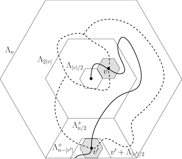
Figure 10: The event that $v$ and $v^{\prime}$ are pivotal for $A_{1}(n)$. The dotted line corresponds to a closed circuit.

Russo’s formula implies

$$\frac{d}{dp}\mathbb{P}_{p}\big{[}A_{1}(n)\big{]}~{}=~{}\sum_{v\in\Lambda_{n}}\mathbb{P}_{p}\big{[}v\text{~{}pivotal for~{}}A_{1}(n)\big{]}.$$ (26)

The site $v$ is pivotal for $A_{1}(n)$ if and only if there are four arms of alternating colors emanating from it, one of the open arms going to the origin, the other to the boundary of the box, and the two closed arms together with the site $v$ forming a circuit around the origin (see Fig 10). Let us treat two cases:

• If $|v|\leq n/2$, where $|v|$ is the graph distance to the origin, the pivotality of the site $v$ implies that the following events hold: $A_{1}(|v|/2)$, $A_{1}(2|v|,n)$ and the translation of $A_{1010}(|v|/2)$ by $v$ (see Fig 10 again). We deduce, using independence, that

  $$\mathbb{P}_{p}\big{[}v\text{~{}pivotal for~{}}A_{1}(n)\big{]} \leq\mathbb{P}_{p}\big{[}A_{1}(|v|/2)\big{]}\mathbb{P}_{p}\big{[}A_{1}(2|v|,n)\big{]}\mathbb{P}_{p}\big{[}A_{1010}(|v|/2)\big{]}$$

  $$\leq C_{1}\mathbb{P}_{p}\big{[}A_{1}(n)\big{]}\mathbb{P}_{p}\big{[}A_{1010}(|v|/2)\big{]},$$

  where in the second line we used (20) twice together with the fact that $\mathbb{P}_{p}\big{[}A_{1}(|v|/2,2|v|)\big{]}\geq C_{0}$ (the latter comes from the crossing estimates (19)). Equations (20) and (25) give

  $$\mathbb{P}_{p}\big{[}A_{1010}(|v|/2)\big{]}\leq C_{2}\left(\frac{2n}{|v|}\right)^{2-c}\mathbb{P}_{p}\big{[}A_{1010}(n)\big{]},$$

  which, when tuned into the previous displayed inequality, leads to

  $$\mathbb{P}_{p}\big{[}v\text{~{}pivotal for~{}}A_{1}(n)\big{]}\leq C_{3}\left(\frac{2n}{|v|}\right)^{2-c}\mathbb{P}_{p}\big{[}A_{1}(n)\big{]}\mathbb{P}_{p}\big{[}A_{1010}(n)\big{]}.$$ (27)

• If $|v|\geq n/2$, the site $v$ is pivotal if the following events hold: $A_{1}(n/2)$, the translation of $A_{1010}(n-|v|)$ by $v$ and the translation of $A^{+}_{010}(n-|v|,n/2)$ by $v$ (see Fig 10 again). We deduce, using independence, that

  $$\mathbb{P}_{p}\big{[}v \text{~{}pivotal for~{}}A_{1}(n)\big{]}$$

  $$\leq\mathbb{P}_{p}\big{[}A_{1}(n/2)\big{]}\mathbb{P}_{p}\big{[}A_{1010}(n-|v|)\big{]}\mathbb{P}_{p}\big{[}A^{+}_{010}(n-|v|,n/2)\big{]}$$

  $$\leq C_{4}\mathbb{P}_{p}\big{[}A_{1}(n)\big{]}\left(n-|v|\right)^{2-c}\mathbb{P}_{p}\big{[}A_{1010}(n)\big{]}\left(\frac{2(n-|v|)}{n}\right)^{2},$$ (28)

  where an argument similar to the previous case was used once again to relate $\mathbb{P}_{p}[A_{1}(n/2)]$ to $\mathbb{P}_{p}\big{[}A_{1}(n)]$ and $\mathbb{P}_{p}[A_{1010}(n-|v|)]$ to $\mathbb{P}_{p}[A_{1010}(n)]$. The bound (23) was used to bound $\mathbb{P}_{p}[A^{+}_{010}(n-|v|,n/2)]$.

Plugging the bounds (27) and (28) into (26), we easily find that for $n\leq L_{p}(\varepsilon)$,

$$\frac{d}{dp}\mathbb{P}_{p}\big{[}A_{1}(n)\big{]}\leq C_{5}\mathbb{P}_{p}\big{[}A_{1}(n)\big{]}\cdot n^{2}\mathbb{P}_{p}\big{[}A_{1010}(n)\big{]}.$$ (29)

We now relate $n^{2}\mathbb{P}_{p}\big{[}A_{1010}(n)\big{]}$ to the derivative of the probability of the event that $[0,n]^{2}$ is crossed horizontally by an open path. Denote this event by $E(n)$. We have

$$\frac{d}{dp}\mathbb{P}_{p}\big{[}E(n)\big{]}~{}=~{}\sum_{v\in\Lambda_{n}}\mathbb{P}_{p}\big{[}v\text{~{}pivotal for~{}}E(n)\big{]}.$$

The site $v$ is pivotal for $E(n)$ if and only if there are four arms of alternating colors emanating from it, the open arms going to the left and the right of the box, and the closed ones to the top and the bottom. Using (21), we find that the probability of $v\in[\frac{n}{3},\frac{2n}{3}]^{2}$ being pivotal for $E(n)$ is larger than a universal constant times the probability of having four arms of alternating colors going from $v$ to the boundary of $[0,n]^{2}$. Since $[0,n]^{2}\subset(v+\Lambda_{2n})$, this implies immediately that

$$\mathbb{P}_{p}\big{[}v\text{~{}pivotal for~{}}E(n)\big{]}\geq\frac{1}{C_{6}}\mathbb{P}_{p}\big{[}A_{1010}(2n)\big{]}\geq\frac{1}{C_{7}}\mathbb{P}_{p}\big{[}A_{1010}(n)\big{]}.$$

Once again, quasi-multiplicativity was used in a crucial way in order to obtain the last inequality. By summing on vertices $v$ in $[\frac{n}{3},\frac{2n}{3}]^{2}$, we get

$$\frac{d}{dp}\mathbb{P}_{p}\big{[}E(n)\big{]}~{}\geq~{}\frac{1}{9C_{7}}n^{2}\mathbb{P}_{p}\big{[}A_{1010}(n)\big{]}.$$ (30)

Altogether, we find that for $n\leq L_{p}(\varepsilon)$,

$$\frac{d}{dp}\mathbb{P}_{p}\big{[}A_{1}(n)\big{]}\leq C_{5}\mathbb{P}_{p}\big{[}A_{1}(n)\big{]}\cdot n^{2}\mathbb{P}_{p}\big{[}A_{1010}(n)\big{]}\leq 9C_{5}C_{7}\mathbb{P}_{p}\big{[}A_{1}(n)\big{]}\frac{d}{dp}\mathbb{P}_{p}\big{[}E(n)\big{]}.$$

Since for $p^{\prime}\in(\frac{1}{2},p)$, $L_{p^{\prime}}(\varepsilon)\geq L_{p}(\varepsilon)$, we deduce that

$$\log\mathbb{P}_{p}\big{[}A_{1}(n)\big{]}-\log\mathbb{P}_{\!\frac{1}{2}}\big{[}A_{1}(n)\big{]}~{} \leq~{}C_{8}\int_{1/2}^{p}\frac{d}{dp^{\prime}}\mathbb{P}_{p^{\prime}}\big{[}E(n)\big{]}~{}dp^{\prime}$$

$$=C_{8}(\mathbb{P}_{p}[E(n)]-\mathbb{P}_{\!\frac{1}{2}}[E(n)])\leq C_{8},$$

which is the claim.

The same reasoning can be applied when $p<\frac{1}{2}$ and for any sequence $\sigma$. The main step is to get (29) with $1$ replaced by $\sigma$, the end of the proof being the same. In order to obtain this inequality, one harnesses a generalization of Russo’s formula; we refer to [Nol08, Theorem 26] for a complete exposition. ∎

4.4 Near-critical exponents

It is now time to relate arm-exponents to near-critical ones. The goal of this section is to prove the following:

Theorem 4.8 (Kesten [Kes87]).

Let $p_{0}\in(0,1)$ and $\varepsilon>0$ small enough. There exist $c,C\in(0,\infty)$ such that for every $p\in(\frac{1}{2},p_{0})$,

$$c~{}\leq~{}(p-1/2)L_{p}(\varepsilon)^{2}\mathbb{P}_{\!\frac{1}{2}}\big{[}A_{1010}(L_{p}(\varepsilon))\big{]}~{}\leq~{}C,$$

$$c\mathbb{P}_{\!\frac{1}{2}}\big{[}A_{1}(L_{p}(\varepsilon))\big{]}~{}\leq~{}\theta(p)~{}\leq~{}C\mathbb{P}_{\!\frac{1}{2}}\big{[}A_{1}(L_{p}(\varepsilon))\big{]}.$$

Note that we reached our original goal since Theorem 1.5 follows readily from Theorems 3.4 and 4.8. Indeed, Theorem 3.4 gives that $\mathbb{P}_{\!\frac{1}{2}}[A_{1010}(n)]=n^{-5/4+o(1)}$ and $\mathbb{P}_{\!\frac{1}{2}}[A_{1}(n)]=n^{-5/48+o(1)}$. Theorem 4.8 implies that $\theta(p)=(p-1/2)^{5/36+o(1)}$, which is exactly the claim of Theorem 1.5.

More generally, if we only assume the existence of $\alpha_{1}$ and $\alpha_{4}$ such that $\mathbb{P}_{\!\frac{1}{2}}[A_{1010}(n)]=n^{-\alpha_{4}+o(1)}$ and $\mathbb{P}_{\!\frac{1}{2}}[A_{1}(n)]=n^{-\alpha_{1}+o(1)}$, the previous statement implies the existence of $\nu$ and $\beta$ such that $L_{p}(\varepsilon)=(p-1/2)^{-\nu+o(1)}$ and $\theta(p)=(p-1/2)^{\beta+o(1)}$. Furthermore, $(2-\alpha_{4})\nu=1$ and $\beta=\alpha_{1}\nu$. This connection between different critical exponents is called a scaling relation.

Proof of Theorem 4.8.

In the proof, $C_{1},C_{2},\dots$ are constants in $(0,\infty)$ depending on $p_{0}$ and $\varepsilon$ only. Let us deal with the second displayed equation first. Let $L_{p}=L_{p}(\varepsilon)$. On the one hand, it is straightforward that $\theta(p)=\mathbb{P}_{p}(0\leftrightarrow\infty)\leq\mathbb{P}_{p}[A_{1}(L_{p})]\leq C_{1}\mathbb{P}_{\!\frac{1}{2}}[A_{1}(L_{p})]$ thanks to Theorem 4.7.

Since a circuit surrounding $\Lambda_{L_{p}}$ has length at least $L_{p}=L_{1-p}$, Proposition 4.1 implies that $\mathbb{P}_{p}[A_{1}(L_{p},n)]\geq C_{2}$ for any $n\geq L_{p}$. Quasi-multiplicativity and Theorem 4.7 imply

$$\mathbb{P}_{p}[A_{1}(n)]\geq\mathbb{P}_{p}[A_{1}(L_{p})]\mathbb{P}_{p}[A_{1}(L_{p},n)]\geq C_{3}\mathbb{P}_{p}[A_{1}(L_{p})]\geq C_{4}\mathbb{P}_{\!\frac{1}{2}}[A_{1}(L_{p})].$$

The claim follows by letting $n$ go to infinity.

We now turn to the first displayed equation. The right-hand inequality is a fairly straightforward consequence of (30) and Theorem 4.7. Indeed, set $E(L_{p})$ be the event that $[0,L_{p}]^{2}$ is crossed horizontally by an open path. Since $L_{p^{\prime}}\geq L_{p}$ for $\frac{1}{2}<p^{\prime}\leq p$, we find that

$$1 \geq\mathbb{P}_{p}[E(L_{p})]-\mathbb{P}_{\!\frac{1}{2}}[E(L_{p})]=\int_{\frac{1}{2}}^{p}\frac{d}{dp^{\prime}}\mathbb{P}_{p^{\prime}}[E(L_{p})]dp^{\prime}$$

$$\geq C_{5}\int_{\frac{1}{2}}^{p}L_{p}^{2}\mathbb{P}_{p^{\prime}}[A_{1010}(L_{p})]dp^{\prime}\geq C_{6}\int_{\frac{1}{2}}^{p}L_{p}^{2}\mathbb{P}_{\!\frac{1}{2}}[A_{1010}(L_{p})]dp^{\prime}$$

$$=C_{7}(p-\textstyle\frac{1}{2})L_{p}^{2}\mathbb{P}_{\!\frac{1}{2}}[A_{1010}(L_{p})].$$

The first equality is due to Russo’s formula. The next two steps are due to (30) followed by Theorem 4.7.

Let us turn to the second inequality of the first displayed equation. Consider the torus $\mathbb{T}_{n}$ of size $n$, which can be seen as $\mathbb{R}^{2}$ quotiented by the following equivalence relation: $(x,y)\sim(x^{\prime},y^{\prime})$ iff $n$ divides $x-x^{\prime}$ and $y-y^{\prime}$. The first homology group of $\mathbb{T}_{n}$ is isomorphic to $\mathbb{Z}^{2}$. Let $[\gamma]\in\mathbb{Z}^{2}$ be the homology class of a circuit $\gamma$.

Let $\mathbb{T}_{n}$ be the image of $\mathbb{T}$ by the canonical projection. A circuit of vertices in $\mathbb{T}$ can be identified to the circuit in $\mathbb{T}_{n}$ created by joining neighboring vertices by a segment of length $1$. Let $F(n)$ be the event that there exists a circuit of open vertices on $\mathbb{T}_{n}$ whose homology class in $\mathbb{Z}^{2}$ has non-zero first coordinate, or in other words, which is winding around $\mathbb{T}_{n}$ “in the vertical direction”.

If $v$ is pivotal for $F(L_{p})$, there are necessarily four paths of alternating colors going to distance $L_{p}/2$ from $v$. Hence,

$$\frac{d}{dp^{\prime}}\mathbb{P}_{p^{\prime}}[F(L_{p})]\leq L_{p}^{2}\mathbb{P}_{p^{\prime}}[A_{1010}(L_{p}/2)]\leq C_{8}L_{p}^{2}\mathbb{P}_{\!\frac{1}{2}}[A_{1010}(L_{p})]$$

by quasi-multiplicativity and Theorem 4.7. By duality, one easily obtain that $\mathbb{P}_{\!\frac{1}{2}}[F(L_{p})]\leq 1/2$. Now, the definition of $L_{p}$ together with a RSW-type argument implies that $\mathbb{P}_{p}[F(L_{p})]$ is larger than $\frac{3}{4}$ if $\varepsilon$ is chosen small enough. Indeed, one can use a construction involving crossings in long rectangles. As a consequence,

$$\tfrac{1}{4}\leq\mathbb{P}_{p}(F(L_{p}))-\mathbb{P}_{\!\frac{1}{2}}(F(L_{p}))=\int_{\frac{1}{2}}^{p}\frac{d}{dp^{\prime}}\mathbb{P}_{p^{\prime}}[F(L_{p})]dp^{\prime}\leq C_{9}(p-\textstyle\frac{1}{2})L_{p}^{2}\mathbb{P}_{\!\frac{1}{2}}[A_{1010}(L_{p})]$$

hence finishing the proof.

∎

5 A few open questions

Percolation on the triangular lattice

Site percolation on the triangular lattice is now very well understood, yet several questions remain open. We select three of them.

We know the behavior of most thermodynamical quantities (the cluster density $\theta$, the truncated mean-cluster size $\chi(p)=(p-1/2)^{-\gamma+o(1)}$ as $p\rightarrow p_{c}$, the two-point functions $\mathbb{P}_{\!\frac{1}{2}}(0\leftrightarrow x)=|x|^{-\eta+o(1)}$ as $x\rightarrow\infty$ and many others). Nevertheless, the behavior of the following fundamental quantity remains unproved:

Question 1.

Prove that the mean number of clusters per site $\kappa(p)=\mathbb{E}_{p}(|C|^{-1})$ behaves like $|1/2-p|^{2+\alpha+o(1)}$, where $C$ is the cluster at the origin and $\alpha=-2/3$.

Interestingly, the critical exponent for $j\neq 1$ disjoint arms of the same color is not equal to the polychromatic arms exponent [BN10]. A natural open question is to compute these exponents:

Question 2.

Compute the monochromatic exponents.

Even the existence of the exponents in the discrete model is not completely understood, because we miss estimates up to constants:

Question 3.

Refine the error term in the arm probabilities from $(n/N)^{\alpha_{j}+o(1)}$ to $(n/N)^{\alpha_{j}}\Theta(1)$.

A result in this direction was obtained in [MNW12] for a half-plane arm-event as a byproduct of a quantitative Cardy’s formula (see also [BCL12] for another quantitative version of Cardy’s formula).

Percolation on other graphs

Conformal invariance has been proved only for site percolation on the triangular lattice. In physics, it is conjectured that the scaling limit of percolation should be universal, meaning that it should not depend on the lattice. For instance, interfaces of bond-percolation on the square lattice at criticality (when the bond-parameter is 1/2) should also converge to ${\mathrm{SLE}}(6)$.

Question 4.

Prove conformal invariance for critical percolation on another planar lattice.

Some progress has been made in [BCL10]. For general graphs, the question of embedding the graph becomes crucial. Indeed, if one embeds the square lattice by gluing long rectangles, then the model will not be rotationally invariant. We refer to [Bef08b] for further details on the subject.

Question 5.

For a general lattice, how may one construct a natural embedding on which percolation is conformally invariant in the scaling limit?

In order to understand universality, a natural class of lattices consists in those for which box crossings probabilities can be studied. Note that proofs of crossing estimates (Corollary 2.3) often invoke some symmetry (rotational invariance for instance) as well as strict planarity, but neither of these seem to be absolutely needed. A proof valid for lattices without one of these properties would be of great significance:

Question 6.

Prove crossing estimates for critical percolation on all planar (and possibly quasi-isometric to planar) lattices.

Let us mention that an important step towards the case of general lattices was accomplished in [GM11a, GM11b, GM12], where critical anisotropic percolation models on the hexagonal, triangular and square lattices is studied.

Percolation in high dimension is well understood (see e.g. [HS94] and references therein), thanks to the so-called triangle condition and the associated lace-expansion techniques. In particular, several critical exponents have been derived (including recently the arm exponents [KN09]) and $\theta(p_{c})$ has been proved to be equal to $0$. In intermediate dimensions, the critical phase is not understood. For instance, one of the main conjectures in probability is to prove that $\theta(p_{c})=0$ for bond percolation on $\mathbb{Z}^{3}$. Even weakening of this conjecture seems to be very hard. For instance, the same question on the graph $\mathbb{Z}^{2}\times\{0,\dots,k\}$ has only been solved very recently (see [DNS12] for site percolation in the case $k=1$, and [DCST13] for the general case).

Other two-dimensional models of statistical physics

Conformal invariance (for instance of crossing probabilities) is not restricted to percolation (see [Smi06, Smi10] and references therein). It should hold for a wide class of two-dimensional lattice models at criticality. Among natural generalizations of percolation, we mention the class of random-cluster models and of loop $O(n)$-models (including the Ising model and the self-avoiding walk). The only three models in this family for which conformal invariance has been proved are the Ising model (the $O(n)$-model with $n=1$), the $q\!=\!2$ random cluster model (which is a geometric representation of the Ising model), and the uniform spanning tree.

Question 7.

Prove conformal invariance of another two-dimensional critical lattice model of percolation type.

Acknowledgments

The authors were supported by the ANR grants BLAN06-3-134462 and MAC2 10-BLAN-0123, the EU Marie-Curie RTN CODY, the ERC AG CONFRA, as well as by the Swiss FNS.

References

- [AB99] M. Aizenman and A. Burchard, Hölder regularity and dimension bounds for random curves, Duke Math. J. 99 (1999), no. 3, 419–453.
- [BB07] N. Berger and M. Biskup, Quenched invariance principle for simple random walk on percolation clusters, Probab. Theory Related Fields 137 (2007), no. 1, 83–120.
- [BCL10] I. Binder, L. Chayes, and H. K. Lei, On convergence to I: conformal invariance for certain models of the bond-triangular type, J. Stat. Phys. 141 (2010), no. 2, 359–390.
- [BCL12] I. Binder, L. Chayes, and H. K. Lei, On the Rate of Convergence for Critical Crossing Probabilities, ArXiv e-prints 1210.1917 (2012).
- [BDC12] V. Beffara and H. Duminil-Copin, The self-dual point of the two-dimensional random-cluster model is critical for , PTRF 153 (2012), page 511.
- [Bef04] V. Beffara, Hausdorff dimensions for SLE6, Ann. Probab. 32 (2004), no. 3B, 2606–2629.
- [Bef07] , Cardy’s formula on the triangular lattice, the easy way, Universality and renormalization, Fields Inst. Commun., vol. 50, Amer. Math. Soc., 2007, pp. 39–45.
- [Bef08a] , The dimension of the SLE curves, Ann. Probab. 36 (2008), no. 4, 1421–1452.
- [Bef08b] , Is critical 2d percolation universal?, In and Out of Equilibrium 2 (2008), 31–58.
- [BH57] S. R. Broadbent and J.M. Hammersley, Percolation processes i. crystals and mazes, Math. Proceedings of the Cambridge Philosophical Society 53 (1957), no. 03, 629–641.
- [BKK+92] J. Bourgain, J. Kahn, G. Kalai, Y. Katznelson, and N. Linial, The influence of variables in product spaces, Israel J. Math. 77 (1992), no. 1-2, 55–64.
- [BN10] V. Beffara and P. Nolin, On monochromatic arm exponents for 2d critical percolation, To appear, 2010.
- [BPZ84a] A. A. Belavin, A. M. Polyakov, and A. B. Zamolodchikov, Infinite conformal symmetry in two-dimensional quantum field theory, Nuclear Phys. B 241 (1984), no. 2, 333–380.
- [BPZ84b] , Infinite conformal symmetry of critical fluctuations in two dimensions, J. Statist. Phys. 34 (1984), no. 5-6, 763–774.
- [BR06a] B. Bollobás and O. Riordan, The critical probability for random Voronoi percolation in the plane is 1/2, Probab. Theory Related Fields 136 (2006), no. 3, 417–468.
- [BR06b] , Percolation, Cambridge University Press, New York, 2006.
- [BR06c] , Percolation, Cambridge Univ Pr, 2006.
- [BR06d] , A short proof of the Harris–Kesten theorem, Bull. London Math. Society 38 (2006), no. 3, 470.
- [Car92] J. L. Cardy, Critical percolation in finite geometries, J. Phys. A 25 (1992), no. 4, L201–L206.
- [CN06] F. Camia and C. M. Newman, Two-dimensional critical percolation: the full scaling limit, Comm. Math. Phys. 268 (2006), no. 1, 1–38.
- [CN07] , Critical percolation exploration path and SLE6: a proof of convergence, Probab. Theory Related Fields 139 (2007), no. 3-4, 473–519.
- [DCST13] H. Duminil-Copin, V. Sidoravicius, and V. Tassion, Absence of percolation for critical bernoulli percolation on planar slabs, preprint, 2013.
- [DNS12] M. Damron, C. M. Newman, and V. Sidoravicius, Absence of site percolation at criticality in , ArXiv e-prints 1211.4138 (2012).
- [DSB03] A. Desolneux, B. Sapoval, and A. Baldassarri, Self-organized percolation power laws with and without fractal geometry in the etching of random solids, Arxiv preprint cond-mat/0302072, 2003.
- [FK96] E. Friedgut and G. Kalai, Every monotone graph property has a sharp threshold, Proceedings of the American Math. Society 124 (1996), no. 10, 2993–3002.
- [FKG71] C. M. Fortuin, P. W. Kasteleyn, and J. Ginibre, Correlation inequalities on some partially ordered sets, Comm. Math. Phys. 22 (1971), 89–103.
- [Fri04] E. Friedgut, Influences in product spaces: KKL and BKKKL revisited, Combinatorics, Probability and Computing 13 (2004), no. 01, 17–29.
- [Gar10] C. Garban, Oded Schramm’s contributions to noise sensitivity, 2010, To appear in the Ann. Probab. volume in honor of Oded Schramm.
- [Geo88] H.-O. Georgii, Gibbs measures and phase transitions, de Gruyter Studies in Mathematics, vol. 9, Walter de Gruyter & Co., Berlin, 1988.
- [GM11a] G. R. Grimmett and I. Manolescu, Inhomogeneous bond percolation on square, triangular, and hexagonal lattices, 2011, to appear in Ann. Probab.
- [GM11b] , Universality for bond percolation in two dimensions, 2011, preprint, arXiv:1108.2784.
- [GM12] , Bond percolation on isoradial graphs, arXiv preprint arXiv:1204.0505 (2012).
- [GPS10] C. Garban, G. Pete, and O. Schramm, The Fourier spectrum of critical percolation, Acta Math. 205 (2010), no. 1, 19–104.
- [Gri99] G. Grimmett, Percolation, Springer Verlag, 1999.
- [Gri06] G. R. Grimmett, The random-cluster model, Grundlehren der Mathematischen Wissenschaften [Fundamental Principles of Math. Sciences], vol. 333, Springer-Verlag, Berlin, 2006.
- [Gri10] , Probability on graphs, Institute of Math. Statistics Textbooks, vol. 1, Cambridge University Press, Cambridge, 2010.
- [Har60] T.E. Harris, A lower bound for the critical probability in a certain percolation process, Math. Proceedings of the Cambridge Philosophical Society 56 (1960), no. 01, 13–20.
- [HS94] T. Hara and G. Slade, Mean-field behaviour and the lace expansion, NATO ASI Series C Math. and Physical Sciences-Advanced Study Institute 420 (1994), 87–122.
- [Kes80] H. Kesten, The critical probability of bond percolation on the square lattice equals , Comm. Math. Phys. 74 (1980), no. 1, 41–59.
- [Kes82] , Percolation theory for mathematicians, Boston, 1982.
- [Kes86] , The incipient infinite cluster in two-dimensional percolation, Probab. Theory Related Fields 73 (1986), no. 3, 369–394.
- [Kes87] , Scaling relations for D-percolation, Comm. Math. Phys. 109 (1987), no. 1, 109–156.
- [KKL88] J. Kahn, G. Kalai, and N. Linial, The influence of variables on Boolean functions, Proceedings of 29th Symposium on the Foundations of Computer Science, Computer Science publisher, 1988.
- [KN09] G. Kozma and A. Nachmias, The Alexander-Orbach conjecture holds in high dimensions, Invent. Math. 178 (2009), no. 3, 635–654.
- [KS06] G. Kalai and S. Safra, Threshold phenomena and influence, Oxford University Press, 2006.
- [KS10] A. Kemppainen and S. Smirnov, Random curves, scaling limits and Loewner evolutions., in preparation, 2010.
- [Lan99] S. Lang, Complex analysis, vol. 103, Springer Verlag, 1999.
- [Law05] G. F. Lawler, Conformally invariant processes in the plane, Math. Surveys and Monographs, vol. 114, American Math. Society, Providence, RI, 2005.
- [LPSA94] R. Langlands, P. Pouliot, and Y. Saint-Aubin, Conformal invariance in two-dimensional percolation, Bull. Amer. Math. Soc. (N.S.) 30 (1994), no. 1, 1–61.
- [LSW01a] G. Lawler, O. Schramm, and W. Werner, Values of Brownian intersection exponents. I. Half-plane exponents, Acta Math. 187 (2001), no. 2, 237–273.
- [LSW01b] , Values of Brownian intersection exponents. II. Plane exponents, Acta Math. 187 (2001), no. 2, 275–308.
- [LSW02] , One-arm exponent for critical 2D percolation, Electron. J. Probab. 7 (2002), no. 2, 13 pp. (electronic).
- [LSW04] G. F. Lawler, O. Schramm, and W. Werner, Conformal invariance of planar loop-erased random walks and uniform spanning trees, Ann. Probab. 32 (2004), no. 1B, 939–995.
- [MNW12] D. Mendelson, A. Nachmias, and S. S. Watson, Rate of Convergence for Cardy’s Formula, ArXiv e-prints 1210.4201 (2012).
- [MP07] P. Mathieu and A. Piatnitski, Quenched invariance principles for random walks on percolation clusters, Proceedings of the Royal Society A: Math., Physical and Engineering Science 463 (2007), no. 2085, 2287.
- [Nol08] P. Nolin, Near-critical percolation in two dimensions, Electron. J. Probab. 13 (2008), no. 55, 1562–1623.
- [Rei00] D. Reimer, Proof of the van den Berg-Kesten conjecture, Combinatorics Probability and Computing 9 (2000), no. 1, 27–32.
- [RS05] S. Rohde and O. Schramm, Basic properties of SLE, Ann. of Math. (2) 161 (2005), no. 2, 883–924.
- [Rus78] L. Russo, A note on percolation, Z. Wahrscheinlichkeitstheorie und Verw. Gebiete 43 (1978), no. 1, 39–48.
- [Sch00] O. Schramm, Scaling limits of loop-erased random walks and uniform spanning trees, Israel J. Math. 118 (2000), 221–288.
- [Smi01] S. Smirnov, Critical percolation in the plane: conformal invariance, Cardy’s formula, scaling limits, C. R. Acad. Sci. Paris Sér. I Math. 333 (2001), no. 3, 239–244.
- [Smi06] , Towards conformal invariance of 2D lattice models, International Congress of Mathematicians. Vol. II, Eur. Math. Soc., Zürich, 2006, pp. 1421–1451.
- [Smi10] , Conformal invariance in random cluster models. I. Holomorphic fermions in the Ising model, Ann. of Math. (2) 172 (2010), no. 2, 1435–1467.
- [SRG85] B. Sapoval, M. Rosso, and J. F. Gouyet, The fractal nature of a diffusion front and the relation to percolation, Journal de Physique Lettres 46 (1985), no. 4, 149–156.
- [SS10] O. Schramm and J. Steif, Quantitative noise sensitivity and exceptional times for percolation, Ann. Math. 171 (2010), no. 2, 619–672.
- [Sun11] N. Sun, Conformally invariant scaling limits in planar critical percolation, Probability Surveys 8 (2011).
- [SW78] P. D. Seymour and D. J. A. Welsh, Percolation probabilities on the square lattice, Ann. Discrete Math. 3 (1978), 227–245, Advances in Graph Theory (Cambridge Combinatorial Conf., Trinity College, Cambridge, 1977).
- [SW01] S. Smirnov and W. Werner, Critical exponents for two-dimensional percolation, Math. Res. Lett. 8 (2001), no. 5-6, 729–744.
- [SW10a] S. Sheffield and W. Werner, Conformal loop ensembles: Construction via loop-soups, Arxiv preprint arXiv:1006.2373 (2010), 21.
- [SW10b] , Conformal loop ensembles: The Markovian characterization, Arxiv preprint arXiv:1006.2374 (2010), 60.
- [vdBK85] J. van den Berg and H. Kesten, Inequalities with applications to percolation and reliability, Journal of applied probability (1985), 556–569.
- [Wer04] W. Werner, Random planar curves and Schramm-Loewner evolutions, Lecture Notes in Mathematics 1840 (2004), 107–195.
- [Wer05] , Conformal restriction and related questions, Probability Surveys 2 (2005), 145–190.
- [Wer09a] , Percolation et modèle d’Ising, Cours Spécialisés [Specialized Courses], vol. 16, Société Mathématique de France, Paris, 2009.
- [Wer09b] Wendelin Werner, Lectures on two-dimensional critical percolation, Statistical mechanics, IAS/Park City Math. Ser., vol. 16, Amer. Math. Soc., 2009, pp. 297–360.