Holography at work for nuclear and hadron physics
Youngman Kim and Deokhyun Yi

Asia Pacific Center for Theoretical Physics and Department of Physics, Pohang University of Science and Technology, Pohang, Gyeongbuk 790-784, Korea

The purpose of this review is to provide basic ingredients of holographic QCD to non-experts in string theory and to summarize its interesting achievements in nuclear and hadron physics. We focus on results from a less stringy bottom-up approach and review a stringy top-down model with some calculational details.

1 Introduction

The approaches based on the Anti de Sitter/conformal field theory (AdS/CFT) correspondence [1, 2, 3] find many interesting possibilities to explore strongly interacting systems. The discovery of D-branes in string theory [4] was a crucial ingredient to put the correspondence on a firm footing. Typical examples of the strongly interacting systems are dense baryonic matter, stable/unstable nuclei, strongly interacting quark gluon plasma, and condensed matter systems. The morale is to introduce an additional space, which roughly corresponds to the energy scale of 4D boundary field theory, and try to construct a 5D holographic dual model that captures certain non-perturbative aspects of strongly coupled field theory, which are highly non-trivial to analyze in conventional quantum field theory based on perturbative techniques. There are in general two different routes to modeling holographic dual of quantum chromodynamics (QCD). One way is a top-down approach based on stringy D-brane configurations. The other way is so-called a bottom-up approach to a holographic, in which a 5D holographic dual is constructed from QCD. Despite the fact that this bottom-up approach is somewhat ad hoc, it reflects some important features of the gauge/gravity duality and is rather successful in describing properties of hadrons. However, we should keep in mind that a usual simple, tree-level analysis in the holographic dual model, both top-down and bottom-up, is capturing the leading $N_{c}$ contributions, and we are bound to suffer from sub-leading corrections.

The goal of this review is twofold. First, we will assemble results mostly from simple bottom-up models in nuclear and hadron physics. Surely we cannot have them all here. We will devote to selected physical quantities discussed in the bottom-up model. The selection of the topics is based on authors’ personal bias. Second, we present some basic materials that might be useful to understand some aspects of AdS/CFT and D-brane models. We will focus on the role of the AdS/CFT in low energy QCD. Although the correspondence between QCD and gravity theory is not known, we can obtain much insights on QCD by the gauge/gravity duality.

We organize this review as follows. Section 2 reviews the gauge/gravity. Section 3 briefly discuss developments of holographic QCD and demonstrates how to build up a bottom-up model using the AdS/CFT dictionary. After discussing the gauge/gravity duality and modeling in the bottom-up approach, we proceed with selected physical quantities. In each section, we show results mostly from the bottom-up approach and list some from the top-down model. Section 4 deals with vacuum condensates of QCD in holographic QCD. We will mainly discuss the gluon condensate and the quark-gluon mixed condensate. Section 5 collects some results on hadron spectroscopy and form factors from the bottom-up model. Contents are glueballs, light mesons, heavy quarkonium, and hadron form-factors. Section 6 is about QCD at finite temperature and density. We consider QCD phase transition and dense matter. Section 7 is devoted to some general remarks on holographic QCD and to list a few topics that are not discussed properly in this article. Due to our limited knowledge, we are not able to cover all interesting works done in holographic QCD. To compensate this defect partially, we will list some recent review articles on holographic QCD.

In Appendix, we look back on some basic materials that might be useful for non-experts in string theory to work in holographic QCD. A: we review the relation between the bulk mass and boundary operator dimension. B: we present a D3/D7 model and axial U(1) symmetry in the model. C: we discuss non-Abelian chiral symmetry based on D4/D8/$\overline{\rm D8}$ model. D&E: we describe how to calculate the Hawking temperature of an AdS black hole. F: we encapsulate the Hawking-Page transition and sketch how to calculate Polyakov loop expectation value in thermal AdS and AdS black hole.

We close this section with a cautionary remark. Though it is tempting to argue that holographic QCD is dual to real QCD, what we mean by QCD here might be mostly QCD-like or a cousin of QCD.

2 Introduction to the AdS/CFT correspondence

The AdS/CFT correspondence, first suggested by Maldacena [1], is a duality between gravity theory in anti de Sitter space (AdS) background and conformal field theory (CFT). The original conjecture states that there is a correspondence between a weakly coupled gravity theory (type IIB string theory) on $AdS_{5}\times S^{5}$ and the strongly coupled ${\cal N}=4$ supersymmetric Yang-Mills theory on the four-dimensional boundary of $AdS_{5}$. The strings reside in a higher-dimensional curved spacetime and there exists some well-defined mapping between the objects in the gravity side and and the dual objects in the four-dimensional gauge theory. Thus, the conjecture allows the use of non-perturbative methods for strongly coupled theory through its gravity dual.

2.1 D$p$ brane dynamics

The duality emerges from a careful consideration of the D-brane dynamics. A D$p$ brane sweeps out $(p+1)$ world-volume in spacetime. Introducing D branes gives open string modes whose endpoints lie on the D branes and the open string spectrum consists of a finite number of massless modes and also an infinite tower of massive modes. The open string end points can move only in the parallel $(p+1)$ directions of the brane, see Figure 1(a), and a D$p$ brane can be seen as a point along its transverse directions. The dynamics of the D$p$ brane is described by the Dirac-Born-Infeld (DBI) action [5] and Chern-Simons term,

$$S_{D_{p}}=-T_{p}\int d^{p+1}x\,e^{-\phi}\sqrt{-{\rm det}\left(P[g]_{ab}+2\pi\alpha^{\prime}F_{ab}\right)}+S_{CS}$$ (2.1)

with a dilaton $e^{-\phi}$. Here $g_{ab}$ is the induced metric on $D_{p}$. $P$ denotes the pullback and $F_{ab}$ is the world-volume field strength. $T_{p}$ is the tension of the brane which has the form

$$T_{p}=\frac{1}{(2\pi)^{p}g_{s}l_{s}^{p+1}}=\frac{1}{(2\pi)^{p}g_{s}\alpha^{\prime(p+1)/2}}$$ (2.2)

and it is the mass per unit spatial volume. Here $g_{s}$ is the string coupling and $l_{s}$ is the string length. $\alpha^{\prime}$ is the Regge slope parameter and related to the string length scale as $l_{s}=\sqrt{\alpha^{\prime}}$. In general, states in the closed string spectrum contain a finite number of massless modes and an infinite tower of massive modes with masses of order $m_{s}=l_{s}^{-1}=\alpha^{\prime-1/2}$. Thus, at low energies $E\ll m_{s}$, the higher order corrections come in powers of $\alpha^{\prime}E^{2}$ from integrating out the massive string modes. If there are a $N_{c}$ stack of multiple D branes, the open strings between different branes give a non-Abelian $U(N_{c})$ gauge group, see Figure 1(b). In the low energy limit, we can integrate out the massive modes to obtain non-Abelian gauge theory of the massless fields.

           

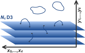
(a) D3 branes sweep $(3\!+\!1)$ dimensions in $(9\!+\!1)$ space time.

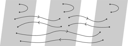
(b) $N_{c}\!=\!3$ stack of D3 branes and all the possible classes of open strings.

Figure 1: The configurations of $N_{c}$ stack of D3 branes in $10d$ spacetime.

Now, we take $p=3$ and consider $N_{c}$ D3 brane stacks in type IIB theory. The low energy effective action of this configuration gives a non-Abelian gauge theory with $U(N_{c})$ gauge group. In addition, this gauge group can be factorized into $U(N_{c})=SU(N_{c})\times U(1)$ and the $U(1)$ part, which describes the center of mass motion of the D3 branes, can be decoupled by the global translational invariance. The remaining subgroup $SU(N_{c})$ describes the dynamics of branes from each other. Therefore we see that in the low energy limit, the massless open string modes on $N_{c}$ stacks of D3-branes constitute ${\cal N}=4$ $SU(N_{c})$ Yang-Mills theory [6] with 16 supercharges in $(3+1)$ spacetime. From (2.1) for $p=3$, we obtain the effective Lagrangian at low energies up to the two derivative order

$${\cal L}=-\frac{1}{4\pi g_{s}}{\mbox{Tr}}\left(\frac{1}{4}F_{\mu\nu}F^{\mu\nu}+\frac{1}{2}D_{\mu}\phi^{i}D^{\mu}\phi^{i}-\frac{1}{4}\left[\phi^{i},\phi^{j}\right]^{2}+\frac{i}{2}\bar{\Psi}^{I}\Gamma^{\mu}D_{\mu}\Psi_{I}-\frac{i}{2}\bar{\Psi}^{I}\Gamma^{i}\left[\phi_{i},\Psi_{I}\right]\right)$$ (2.3)

with a gauge field $A_{\mu}$, six scalar fields $\phi^{i}$ and four Weyl fermions $\Psi^{I}$.

In fact, the original system also contains closed string states. The higher order derivative corrections for the Lagrangian (2.3) come both in powers of $\alpha^{\prime}E^{2}$ from the massive modes and powers of the string coupling $g_{s}N_{c}$ for loop corrections. It is known that the string coupling constant $g_{s}$ is related by the 10-dimensional gravity constant as $G^{(10)}\sim g_{s}^{2}l_{s}^{8}$ and thus the dimensionless string coupling is of order $G^{(10)}E^{8}$, which is negligible in the low energy limit. Therefore, at low energies closed strings are decoupled from open strings and the physics on the $N_{c}$ D3 branes is described by the massless ${\cal N}=4$ super Yang-Mills theory with gauge group $SU(N_{c})$.

2.2 $AdS_{5}\times S^{5}$ geometry

Now we view the same system from a different angle. Since D branes are massive and carry energy and Ramond-Ramond (RR) charge, $N_{c}$ D3 branes deforms the spacetime around them to make a curved geometry. Note that the total mass of a D3 brane is infinite because it occupies the infinite world-volume of its transverse directions, but the tension, or the mass per unit three-volume of the D3 brane

$$T_{3}=1/(2\pi)^{3}g_{s}l_{s}^{4}$$ (2.4)

is finite.

In the flat spacetime, the circumference of the circle surrounding an origin at a distance $r$ is $2\pi r$, and it simply shrinks to zero if one approaches the origin. But if there is a stack of D3 branes, it deforms the spacetime and makes throat geometry along its transverse directions. Thus, near the D3 branes, the radius of a circle around the stack approaches a constant $R$, an asymptotical infinite cylinder structure, or $AdS_{5}\times S^{5}$, see Figure 2(b). The $N_{c}$ D3 brane stack is located at the infinite end of the throat and this infinite end is called the “horizon”. In the near horizon geometry, a D3 brane is surrounded by a five-dimensional sphere $S^{5}$.

     

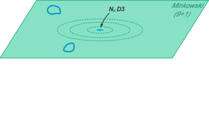
(a) Flat spacetime for $r\gg R$.

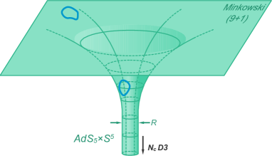
(b) $N_{c}$ D3 branes deform the spacetime.

Figure 2: The two descriptions of the $N_{c}$ D3 configuration.

To be more specific, let us start with type IIB string theory for $p=3$. We find a black hole type solution which is carrying charges with respect to the RR four-form potential. The theory has magnetically charged D3 branes, which are electrically charged under the potential $dA_{4}$ and it is self-dual $*F_{5}=F_{5}$. The low energy effective action is

$$S=\frac{1}{(2\pi)^{7}l_{s}^{8}}\int d^{10}x\sqrt{-g}\left(e^{-2\phi}(R+4(\nabla\varphi)^{2})-\frac{2}{5!}F^{2}_{5}\right)\,.$$ (2.5)

We assume that the metric is spherically symmetric in seven-dimensions with the RR source at the origin, then the $N_{c}$ parameter appears in terms of the five-form field RR-field strength on the five-sphere as

$$\int_{S^{5}}\,*F_{5}=N_{c}$$ (2.6)

where $S^{5}$ is the five-sphere surrounding the source for a four-form field $C_{4}$. Now by using the Euclidean symmetry we get the curved metric solution [7, 8, 9] for the D3 brane

$$ds^{2}=f(r)^{-1/2}\eta^{\mu\nu}dx_{\mu}dx_{\nu}+f(r)^{1/2}\left(dr^{2}+r^{2}\,d\Omega_{5}^{2}\right)\,,$$ (2.7)

where

$$f(r)=1+\frac{R^{4}}{r^{4}}$$ (2.8)

with the radius of the horizon $R$

$$R^{2}=\sqrt{4\pi g_{s}N_{c}}\alpha^{\prime}=\sqrt{4\pi g_{s}N_{c}}l_{s}^{2}\,.$$ (2.9)

$d\Omega_{5}$ is the five-sphere metric. For $r\gg R$ we have $f(r)\simeq 1$ and the spacetime becomes flat with a small correction $R^{4}/r^{4}=4\pi g_{s}N_{c}l_{s}^{4}/r^{4}$. This factor can be interpreted as a gravitational potential since $G^{(10)}\sim g_{s}^{2}l_{s}^{8}$ and $M_{D3}\sim N_{c}T_{3}\sim N_{c}/g_{s}l_{s}^{4}$ thus $R^{4}/r^{4}\sim GM_{D3}/r^{4}$. In the near horizon limit, this gravitational effect become strong and the metric changes into

$$ds^{2}=\frac{r^{2}}{R^{2}}\eta^{\mu\nu}dx_{\mu}dx_{\nu}+\frac{R^{2}}{r^{2}}\left(dr^{2}+r^{2}d\Omega_{5}^{2}\right).$$ (2.10)

This is $AdS_{5}\times S^{5}$.

The geometry by the D3 branes is sketched in Figure 2(b). Far away from the D3 brane stacks, the spacetime is flat $(9+1)$ dimensional Minkowski spacetime and the only modes which survive in the low energy limit are the massless closed string (graviton) multiplets, and they decouple from each other due to weak interactions. On the other hand, close to the D3 branes, the geometry takes the form $AdS_{5}\times S^{5}$ and the whole tower of massive modes exists there. This is because the excitations seen from an observer at infinity are close to the horizon and a closed string mode in a throat should go over a gravitational potential to meet the asymptotic flat region. Therefore, as we focus the lower energy limit, the excitation modes should be originated deeper in the throat, and then they decouple from the ones in the flat region. Thus in the low energy limit the interacting sector lives in $AdS_{5}\times S^{5}$ geometry.

2.3 The gauge/gravity duality

So far, we have considered two seemingly different descriptions of the $N_{c}$ D3 brane configuration. As we mentioned, each of the D3 branes carries the gravitational degrees of freedom in terms of its tension, or the string coupling $g_{s}$ as in (2.4). So the strength of the gravity effect due to $N_{c}$ stacks of D3 branes depends on the parameter $g_{s}N_{c}$.

If $g_{s}N_{c}\ll 1$, from (2.9) we see that $R\ll l_{s}$ and therefore the throat geometry effect is less than string length scale. Thus the spacetime is nearly flat and the fluctuations of the D3 branes are described by open string states. In this regime the string coupling $g_{s}$ is small and the closed strings are decoupled from the open strings. Here the closed string description is inapplicable since one needs to know about the geometry below the string length scale. If we take the low energy limit, the effective theory, which describes the open string modes, is ${\cal N}=4$ super Yang-Mills theory with $SU(N_{c})$ gauge group.

On the other hand, if $g_{s}N_{c}\gg 1$, then the back-reaction of the branes on the background becomes important and spacetime will be curved. In this limit the closed string description reduces to classical gravity which is supergravity theory in the near horizon geometry. Here the open string description is not feasible because $g_{s}N_{c}$ is related with the loop corrections and one has to deal with the strongly coupled open strings. Again, if we take the low energy limit, the interaction is described by the type IIB string theory in the near-horizon geometry, $AdS_{5}\times S^{5}$.

The gauge/gravity correspondence is nothing but the conjecture connecting these two descriptions of $N_{c}$ D3 branes in the low energy limit. It is a duality between the ${\cal N}=4$ super Yang-Mills theory with gauge group $SU(N_{c})$ and the type IIB closed string theory in $AdS_{5}\times S^{5}$, see Figure 3.

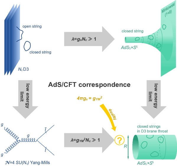
Figure 3: The sketch of the AdS/CFT correspondence.

The relation between the Yang-Mills coupling $g_{YM}$ and the string coupling strength $g_{s}$ is given by

$$g_{YM}^{2}=4\pi g_{s},\qquad(R/l_{s})^{4}=4\pi g_{s}N_{c}$$ (2.11)

Then, the ’t Hooft coupling $\lambda=g_{YM}^{2}N_{c}$ can be expressed in terms of the string length scale

$$\lambda=R^{4}/l_{s}^{4}.$$ (2.12)

Therefore, the dependence of $g_{s}N_{c}$ becomes the question of whether the ’t Hooft coupling is large or small, or the gauge theory is strongly or weakly coupled.

The two descriptions can be viewed as two extremes of $r$. For the sake of convenience, we use the coordinate $z=R^{2}/r$. Then, the $AdS_{5}\times S^{5}$ metric (2.10) becomes

$$ds^{2}=\frac{R^{2}}{z^{2}}\left(\eta^{\mu\nu}dx_{\mu}dx_{\nu}+dz^{2}\right)+R^{2}d\Omega_{5}^{2},$$ (2.13)

which shows the conformal equivalence between $AdS_{5}$ and flat spacetime more clearly. In (2.13), each $z$-slice of $AdS_{5}$ is isometric to four-dimensional Minkowski spacetime. In this coordinate, $z=0$ is the boundary of $AdS_{5}$, where Yang-Mills theory lives, with identifying $x^{\mu}$ as the coordinates of the gauge theory. If $z\rightarrow\infty$, the determinant of the metric goes to zero and it is the Poincaré horizon. Here the factor $R^{2}/z^{2}$ also has some relation with the energy scales. If the gauge theory side has a certain energy scale $E$, the corresponding energy in the gravity side is $(z/R)E$. In order words, a gauge theory object with an energy scale $E$ is involved with a bulk side one localized in the z-direction at $z\sim 1/E$ [1, 10, 11]. Therefore, the UV or high energy limit corresponds to $z\rightarrow 0$ (or $r\rightarrow\infty$) and the IR or low energy limit corresponds to $z\rightarrow\infty$ (or $r\rightarrow 0$).

The operator-field correspondence between operators in the four-dimensional gauge theory and corresponding dual fields in the gravity side was given in [2, 3]. Then the AdS/CFT correspondence can be stated as follows,

$$\left\langle Te^{\int\!d^{4}x\,\phi_{0}(x){\cal O}(x)}\right\rangle_{{\rm CFT}}=Z_{{\rm sugra}}$$ (2.14)

where $\phi_{0}(x)=\phi(x,u\rightarrow\infty)$ and the string theory partition function $Z_{{\rm sugra}}$ at the boundary specified by $\phi_{0}$ has the form

$$Z_{{\rm sugra}}=e^{-S_{{\rm sugra}}\left(\phi(x,u)\right)}\Big{|}_{u\rightarrow\infty}\,.$$ (2.15)

The relation (2.14) implies that the generating functional of gauge-invariant operators in CFT can be matched with the generating functional for tree diagrams in supergravity.

3 Holographic QCD

Ever since the advent of the AdS/CFT correspondence, there have been many efforts, based on the correspondence, to study non-perturbative physics of strongly coupled gauge theories in general and QCD in particular.

Witten proposed [12] that we can extend the correspondence to non-supersymmetric theories by considering the AdS black hole and showed that this supergravity treatment qualitatively well describes strong coupled QCD (or QCD-like) at finite temperature: for instance, the area law behavior of Wilson loops, confinement/deconfinement transition of pure gauge theory through the Hawking-Page transition, and the mass gap for glueball states. In [13] symmetry breaking by expectation values of scalar fields were analyzed in the context of the AdS/CFT correspondence, which is essential to encode the spontaneous breaking of chiral symmetry in a holographic QCD model. Regular supergravity backgrounds with less supersymmetries corresponding to dual confining ${\cal N}=1$ super Yang-Mills theories were proposed in [14, 15]. It has been shown by Polchinski and Strassler [16] that the scaling of high energy QCD scattering amplitudes can be obtained from a gravity dual description in a sliced AdS geometry whose IR cutoff is determined by the mass of the lightest glueball. Important progress towards flavor physics of QCD has been made by adding flavor degrees of freedom in the fundamental representation of a gauge group to the gravity dual description [17]. Chiral symmetry breaking and meson spectra were studied in a nonsupersymmetric gravity model dual to large $N_{c}$ nonsupersymmetric gauge theories [18], where flavor quarks are introduced by a D7-brane probe on deformed AdS backgrounds. Using a D4/D6 brane configuration, the authors of [19] explored the meson phenomenology of large $N_{c}$ QCD together with U(1)_A chiral symmetry breaking. They showed that the chiral condensate scales as $1/m_{q}$ for large $m_{q}$. A remarkable observation made in [19] is that in addition to the confinement/deconfinement phase transition the model exhibits a possibility that another transition set by $T_{fund}$ could happen in deconfined phase, $T>T_{deconf}$, where $T_{deconf}=M_{KK}/(2\pi)$. Since the value of $M_{KK}$ is around $1$ GeV, we can estimate $T_{deconf}\sim 160$ MeV. In this case for $T_{deconf}<T<T_{fund}$ there exist free unbound quarks and meson bound sates of heavy quarks and above $T_{fund}$ the meson states dissociate into free quarks, which in some sense mimics the dissociation of heavy quarkonium in quark-gluon plasma (QGP). However, we should note that meson bound states in Dp/Dq systems are deeply bound, while the heavy quarkonia in QCD are shallow bound states. In this sense the bound state that disappears above $T_{fund}$ could be that of strange quarks rather than charmonium or bottomonium [20].

To attain a realistic gravity dual description of (large $N_{c}$) QCD, non-Abelian chiral symmetry is an essential ingredient together with confinement. Holographic QCD models, which are equipped with the correct structure for the problem, namely, chiral symmetry and confinement, have suggested in top-down and bottom-up approaches. They found to be rather successful for various hadronic observables and for certain processes dominated by large $N_{c}$. Based on a D4/D8/$\overline{\rm D8}$ model, Sakai and Sugimoto studied hadron phenomenology in the chiral limit $m_{q}=0$, and the chiral symmetry breaking geometrically [21, 22]. More phenomenological holographic QCD models were proposed [23, 24, 25]. In [23, 24], chiral symmetry breaking is realized by a non-zero chiral condensate whose value is fitted to meson data from experiments. Hadronic spectra and light-front wave functions were studied in [26] based on the “Light-Front Holography” which maps amplitudes in extra dimension to a Lorentz invariant impact separation variable $\zeta$ in Minkowski space at fixed light-front time. Light-Front Holography has led to many successful applications in hadron physics including light-quark hadron spectra, meson and baryon form factors, the nonperturbative QCD coupling, light-front wave-functions, see [27, 28, 29] for a review on this topic. In [30], a relation between a bottom-up holographic QCD model and QCD sum rules was analyzed.

Now, we demonstrate how to construct a bottom-up holographic QCD model by looking at a low-energy QCD. For illustration purposes, we compare our approach with the (gauged) linear sigma model. The D3/D7 model is summarized in Appendix B with some calculational details. For a review of the linear sigma model, we refer to [31]. Some material in this section is taken from [32]. Suppose we are interested in two-flavor QCD at low energy, roughly below $1$ GeV. In this regime usually we resort to the effective models or theories of QCD for analytic studies since the QCD lagrangian does not help much.

To construct the holographic QCD model dual to two flavor low-energy QCD with chiral symmetry, we first choose relevant fields. To do this, we consider composites of quark fields that have the same quantum numbers with the hadrons of interest. For instance, in the linear sigma model we introduce pion-like and sigma-like fields: $\vec{\pi}\sim\bar{q}\vec{\tau}\gamma^{5}q$ and $\sigma\sim\bar{q}q$, where $\vec{\tau}$ is the Pauli matrix for isospin. In the AdS/CFT dictionary, this procedure may be dubbed operator/field correspondence: one-to-one mapping between gauge-invariant local operators in gauge theory and bulk fields in gravity sides. Then we introduce

$$\bar{q}_{L}\gamma^{\mu}t^{a}q_{L}\leftrightarrow A_{L\mu}^{a}(x,z)\,,$$

$$\bar{q}_{R}\gamma^{\mu}t^{a}q_{R}\leftrightarrow A_{R\mu}^{a}(x,z)\,,$$

$$\bar{q}_{R}^{\alpha}q_{L}^{\beta}\leftrightarrow(2/z)X^{\alpha\beta}(x,z)\,.$$ (3.1)

An interesting point here is that the 5D mass of the bulk field is not a free parameter of the model. This bulk mass is determined by the dimension $\Delta$ and spin $p$ of the dual 4D operator in AdS_d+1. For instance, consider a bulk field $X(x,z)$ dual to $\bar{q}(x)q(x)$. The bulk mass of $X(x,z)$ is given by $m_{X}^{2}=(\Delta-p)(\Delta+p-d)$ with $\Delta=3$, $p=0$ and $d=4$, and so $m_{X}^{2}=-3$. For more details, see Appendix A.

To write down the Lagrangian of the linear sigma model, we consider (global) chiral symmetry of QCD. Since the mass of light quark $\sim 10$ MeV is negligible compared to the QCD scale $\Lambda_{\rm QCD}\sim 200$ MeV, we may consider the exact chiral symmetry of QCD and treat quark mass effect in a perturbative way. Under the axial transformation, $q\rightarrow e^{-i\gamma_{5}\vec{\tau}\cdot\vec{\theta}/2}q$, the pion-like and sigma-like states transform as $\vec{\pi}\rightarrow\vec{\pi}+\vec{\theta}\sigma$ and $\sigma\rightarrow\sigma-\vec{\theta}\cdot\vec{\pi}$. From this, we can obtain terms that respect chiral symmetry such as $\vec{\pi}^{2}+\sigma^{2}$. Similarly we ask the holographic QCD model to respect chiral symmetry of QCD. In AdS/CFT, however, a global symmetry in gauge theory corresponds local symmetry in the bulk, and therefore the corresponding holographic QCD model should posses local chiral symmetry. This way vector and axial-vector fields naturally fit into chiral Lagrangian in the bulk as the gauge boson of the local chiral symmetry.

We keep the chiral symmetry in the Lagrangian since it will be spontaneously broken. Then we should ask how to realize the spontaneous chiral symmetry breaking. In the linear sigma model, we have a potential term like $((\vec{\pi}^{2}+\sigma^{2})-c^{2})^{2}$ that leads to spontaneous chiral symmetry breaking due to a nonzero vacuum expectation value of the scalar field $\sigma$, $\langle\sigma\rangle=c$. In this case the explicit chiral symmetry due to the small quark mass could be mimicked by adding a term $-\epsilon\sigma$ to the potential which induces a finite mass of the pion, $m_{\pi}^{2}\sim\epsilon/c$. In a holographic QCD model, the chiral symmetry breaking is encoded in the vacuum expectation value of a bulk scalar field dual to $\bar{q}q$. For instance in the hard wall model [23, 24], it is given by $\langle X\rangle=m_{q}z+\zeta z^{3}$, where $m_{q}$ and $\zeta$ are proportional to the quark mass and the chiral condensate in QCD. In the D3/D7 model, chiral symmetry breaking can be realized by the embedding solution as shown in Appendix B.

The last step to get to the gravity dual to two flavor low-energy QCD is to ensure the confinement to have discrete spectra for hadrons. The simplest way to realize it might be to truncate the extra dimension at $z=z_{m}$ such that the radial direction $z$ of dual gravity runs from zero to $z_{m}$. Since the radial direction corresponds to an energy scale of a boundary gauge theory, $1/z_{m}$ maps to $\Lambda_{QCD}$.

Putting things together, we could arrive at the following bulk Lagrangian with local SU(2)${}_{\rm L}\times$ SU(2)_R, the hard wall model [23, 24],

$$S_{\rm HW}=\int d^{4}x\int dz\sqrt{g}~{}{\rm Tr}\left[-\frac{1}{4g_{5}^{2}}(F_{L}^{2}+F_{R}^{2})+|DX|^{2}+3|X|^{2}~{}\right],$$ (3.2)

where $D_{\mu}X=\partial_{\mu}X-iA_{L\mu}\,X+iXA_{R\mu}$ and $A_{L,R}=A^{a}_{L,R}t^{a}$ with ${\rm Tr}(t^{a}t^{b})=\frac{1}{2}\delta^{ab}$. The bulk scalar field is defined by $X=X_{0}\,e^{2i\,\pi^{a}t^{a}}$, where $X_{0}\equiv\langle X\rangle$. Here $g_{5}$ is the five dimensional gauge coupling, $g_{5}^{2}=12\pi^{2}/N_{c}$. The background is given by

$$ds^{2}=\frac{1}{z^{2}}(dt^{2}-d{\vec{x}}^{2}-dz^{2})\,,~{}0\leq z\leq z_{m}\,.$$ (3.3)

Instead of the sharp IR cutoff in the hard wall mode, we may introduce a bulk potential that plays a role of a smooth cutoff. In [33], this smooth cutoff is introduced by a factor $e^{-\Phi}$ with $\Phi(z)=z^{2}$ in the bulk action, the soft wall model. The form $\Phi(z)=z^{2}$ in the AdS would ensure the Regge-like behavior of the mass spectrum $m_{n}^{2}\sim n$. The action is given by

$$S_{\rm SW}=\int d^{4}x\int dze^{-\Phi}\sqrt{g}~{}{\rm Tr}\left[-\frac{1}{4g_{5}^{2}}(F_{L}^{2}+F_{R}^{2})+|DX|^{2}+3|X|^{2}~{}\right]\,.$$ (3.4)

Here we briefly show how to obtain the 4D vector meson mass in the soft wall model. The vector field is defined by $V=A_{L}+A_{R}$. With the Kaluza-Klein decomposition $V_{\mu}^{a}(x,z)=g_{5}\sum_{n}v_{n}(z)\rho_{\mu}^{a}(x)$, we obtain

$$\partial_{z}(e^{-B}\partial_{z}v_{n})+m_{n}^{2}e^{-B}v_{n}=0,$$ (3.5)

where $B=\Phi(z)-A(z)=z^{2}+\log z$ in the AdS geometry (3.3). With $v_{n}=e^{B}\psi_{n}$, we transform the equation of motion into the form of a Schrödinger equation

$$\psi_{n}^{{}^{\prime\prime}}-V(z)\psi_{n}=-m_{n}^{2}\psi_{n}\,,$$ (3.6)

where $V(z)=z^{2}+3/(4z^{2})$. Here $m_{n}$ is the mass of the vector resonances, and $\rho$ meson corresponds to $n=0$. The solution is well-known in quantum mechanics and the eigenvalue $m_{n}^{2}$ is given by [33]

$$m_{n}^{2}=4c(n+1),$$ (3.7)

where $c$ is introduced to restore the energy dimension.

The finite temperature could be neatly introduced by a black hole in AdS_d+1, where $d$ is the dimension of the boundary gauge theory. The background is given by

$$ds^{2}=\frac{1}{z^{2}}\left(f(z)dt^{2}-d{\vec{x}}^{2}-\frac{dz^{2}}{f(z)}\right)\,,$$ (3.8)

where $f(z)=1-z^{d}/z_{h}^{d}$. The temperature of the boundary gauge theory is identified with the Hawking temperature of the black hole $T=d/(4\pi z_{h})$. In Appendix D and E, we try to explain in a comprehensive manner how to calculate the Hawking temperature of a black hole.

Now we move on to dense matter. According to the AdS/CFT dictionary, a chemical potential in boundary gauge theory is encoded in the boundary value of the time component of the bulk U(1) gauge field. To be more specific on this, we first consider the chemical potential term in gauge theory,

$${\cal L_{\mu}}=\mu_{q}q^{\dagger}q\,.$$ (3.9)

Then, we introduce a bulk U(1) gauge field $A_{\mu}$ which is dual to $\bar{q}\gamma_{\mu}q$. According to the dictionary, $A_{0}(z\rightarrow 0)\sim c_{1}z^{d-\Delta-p}+c_{2}z^{\Delta-p}$, we have $A_{0}(z\rightarrow 0)\sim\mu_{q}$. In the hard wall model, the solution of the bulk U(1) vector field is given by

$$A_{t}(z)=\mu+\rho z^{2}\,,$$ (3.10)

where $\mu$ and $\rho$ are related to quark chemical potential and quark (or baryon) number density in boundary gauge theory. It is interesting to notice that in chiral perturbation theory, a chemical potential is introduced as the time component of a gauge field by promoting the global chiral symmetry to a local gauge one [34].

4 Vacuum structures

At low energy or momentum scales roughly smaller than $1$ GeV, $r>1$ fm, QCD exhibits confinement and a non-trivial vacuum structure with condensates of quarks and gluons. In this section, we discuss the gluon condensate and quark-gluon mixed condensate.

The gluon condensate $\langle G_{\mu\nu}^{a}G_{a}^{\mu\nu}\rangle$ was first introduced, at zero temperature, in [35] as a measure for nonperturbative physics in QCD. The gluon condensate characterizes the scale symmetry breaking of massless QCD at quantum level. Under the infinitesimal scale transformation

$$x_{\mu}^{\prime}=(1+\delta\lambda)x_{\mu}\,,$$

$$A_{\mu}^{\prime}=(1-\delta\lambda)A_{\mu}\,,$$

$$q^{\prime}=(1-\frac{3}{2}\delta\lambda)q\,,$$ (4.1)

the trace of the energy momentum tensor reads schematically

$$\partial_{\mu}J_{\rm D}^{\mu}=T_{\mu}^{\mu}\simeq-\langle\frac{\alpha_{s}}{\pi}G_{\mu\nu}^{a}G_{a}^{\mu\nu}\rangle\,.$$ (4.2)

Here $J_{\rm D}^{\mu}$ is the dilatation current, $\alpha_{s}$ is the gauge coupling, $T_{\mu\nu}$ is the energy-momentum tensor of QCD. Due to Lorentz invariance, we can write $\langle T_{\mu\nu}\rangle=-\epsilon_{vac}\eta^{\mu\nu}$, where $\epsilon_{vac}$ is the energy of the QCD vacuum. Therefore, the value of the gluon condensate sets the scale of the QCD vacuum energy. In addition, the gluon condensate is important in the QCD sum rule analysis since it enters in the operator product expansion (OPE) of the hadronic correlators [35]. At high temperature, the gluon condensate is useful to study the nonperturbative nature of the QGP. For instance, lattice QCD results on the gluon condensate at finite temperature [36] indicate that the value of the gluon condensate shows a drastic change around $T_{c}$ regardless of the number of quark flavors. The change in the gluon condensate could lead to a dropping of the heavy quarkonium mass around $T_{c}$ [37].

In holographic QCD, the gluon condensate figures in a dilaton profile according to the AdS/CFT since the dilaton is dual to the scalar gluon operator Tr$(G_{\mu\nu}G^{\mu\nu})$. The 5D gravity action with the dilaton is given by

$$S=\gamma\frac{1}{2\kappa^{2}}\int d^{5}x\sqrt{g}\left[{\cal R}+\frac{12}{R^{2}}-\frac{1}{2}\partial_{M}\phi\partial^{M}\phi\right],$$ (4.3)

where $\gamma=+1$ for Minkowski metric, and $\gamma=-1$ for Euclidean signature. We work with Minkowski metric for most cases in this paper. The solution of this system is discovered in [38, 39] by solving the coupled dilaton equation of motion and the Einstein equation:

$$ds^{2}=\left(\frac{R}{z}\right)^{2}\left(\sqrt{1-c^{2}z^{8}}~{}\eta_{\mu\nu}dx^{\mu}dx^{\nu}+dz^{2}\right)\,,$$ (4.4)

and the corresponding dilaton profile is given by

$$\phi(z)=\sqrt{\frac{3}{2}}\log\left(\frac{1+cz^{4}}{1-cz^{4}}\right)+\phi_{0}\,,$$ (4.5)

where $\phi_{0}$ is a constant. At $z=1/c^{1/4}$ there exists a naked singularity that might be resolved in a full string theory consideration. Near the boundary $z\rightarrow 0$,

$$\phi(z)\sim cz^{4}\,.$$ (4.6)

Therefore, $c$ is nothing but the gluon condensate up to a constant. Unfortunately, however, $c$ is an integration constant of the coupled dilaton equation of motion and the Einstein equation and therefore, it will be determined by matching with physical observables. In [39], the value of the gluon condensate is estimated by the glueball mass. An interesting idea based on the circular Wilson loop calculation in gravity side is proposed to calculate the value of the gluon condensate $G_{2}$ $\equiv\langle\frac{\alpha_{s}}{\pi}G_{\mu\nu}^{a}G_{\mu\nu}^{a}\rangle$ [40]. The value is determined to be $G_{2}=0.010\pm 0.0023$ GeV at zero temperature [40]. A phenomenological estimation of the gluon condensate in QCD sum rules gives $\langle\frac{\alpha_{s}}{\pi}G_{\mu\nu}^{a}G_{a}^{\mu\nu}\rangle\simeq 0.012$ GeV⁴ [35].

Now we consider quark-gluon mixed condensate $\langle\bar{q}\sigma_{\mu\nu}G^{\mu\nu}q\rangle$, which can be regarded as an additional order parameter for the spontaneous chiral symmetry breaking since the quark chirality flips via the quark-gluon operator. Thus, it is naturally expressed in terms of the quark condensate as

$$\langle\bar{q}\sigma_{\mu\nu}G^{\mu\nu}q\rangle=m_{0}^{2}\langle\bar{q}q\rangle\,.$$ (4.7)

In [41], an extended hard wall model is proposed to calculate the value of $m_{0}^{2}$. The bulk action of the extended model is given by

$$S\;=\;\int\,d^{5}x\,\sqrt{g}\,\mathrm{Tr}\left[|DX|^{2}+3|X|^{2}-\frac{1}{4g_{5}^{2}}(F_{L}^{2}+F_{R}^{2})+|D\Phi|^{2}-5\Phi^{2}\right],$$ (4.8)

where $\Phi$ is a bulk scalar field dual to the 4D operator on the left-hand-side of Eq. (4.7). Then the chiral condensate and the mixed condensate are encoded in the vacuum expectation value of the two scalar fields.

$$\langle X(x,z)\rangle\;=\;\frac{1}{2}(\hat{m}z+\sigma z^{3}),$$ (4.9)

$$\langle\Phi(x,z)\rangle\;=\;\frac{1}{6}(c_{1}z^{-1}+\sigma_{M}z^{5}),$$ (4.10)

where $c_{1}$ is the source term for the mixed condensate and $\sigma_{M}$ represents the mixed condensate $\sigma_{M}\;=\;\langle\bar{q}_{R}\sigma_{\mu\nu}G^{\mu\nu}q_{L}\rangle$. Taking $c_{1}=0$, a source-free condition to study only spontaneous symmetry breaking, we determine the value of the mixed condensate or $m_{0}^{2}$ by considering various hadronic observables. In this sense the mixed condensate is not calculated but fitted to experimental data like the chiral condensate in the hard wall model. The favored value of the $m_{0}^{2}$ in [41] is $0.72$ GeV². A new method to estimate the value of $m_{0}^{2}$ in is suggested in [42], where a nonperturbative gauge invariant correlator (the nonlocal condensate) is calculated in dual gravity description to obtain $m_{0}^{2}$. With inputs from the slopes for the Regge trajectory of vector mesons and the linear term of the Cornell potential, they obtained $m_{0}^{2}=0.70$ GeV², which is comparable to that from the QCD sum rules, $0.8$ GeV² [43].

5 Spectroscopy and form factors

Any newly proposed models or theories in physics are bound to confront experimental data, for instance hadron masses, decay constants and form factors. In this section, we consider the spectroscopy of the glueball, light meson, heavy quarkonium, and hadron form factors in hard wall model, soft wall model, and their variants.

5.1 Glueballs

Glueballs are made up of gluons with no constituent quarks in them. The glueball states are in general mixed with conventional $\bar{q}q$ states, so in experiments we may observe these mixed states only. Their existence was expected from the early days of QCD [44, 45]. For theoretical and experimental status of glueballs, we refer to [46, 47].

The spectrum of glueballs is one of the earliest QCD quantities calculated based on the AdS/CFT duality. In [12], Witten confirmed that the existence of the mass gap in the dilaton equation of motion on a black hole background, implying a discrete glueball spectrum with a finite gap. Extensive studies on the glueball spectrum were done in [48, 49] and there also comparisons between the supergravity results and lattice gauge theory results were made.

Now we consider a scalar glueball ($0^{++}$) on ${\bf R}^{3}\times{\bf S}^{1}$ as an example [48]. When the radius of the circle ${\bf S}^{1}$ is very small $R\rightarrow 0$, only the gauge degrees of freedom remains and the gauge theory is effectively the same as pure QCD₃ [12, 48]. Using the operator/field correspondence, we first find operators that have the quantum numbers with glueball states of interest and then introduce a corresponding bulk field to obtain the glueball masses. In this case we are to solve an equation of motion for a bulk scalar field $\phi$, which is dual to tr$F^{2}$ in the AdS₅ Euclidean black hole background. The equation of motion for $\phi$ is given by

$$\partial_{\mu}\left(\sqrt{g}\partial_{\nu}\phi g^{\mu\nu}\right)=0\,,$$ (5.1)

and the metric is

$$ds^{2}=\left(\rho^{2}-\frac{b^{4}}{\rho^{2}}\right)^{-1}d\rho^{2}+\left(\rho^{2}-\frac{b^{4}}{\rho^{2}}\right)d\tau^{2}+\rho^{2}+(d\vec{x})^{2}+d\Omega_{5}^{2}\,,$$ (5.2)

where $\tau$ is for the compactified imaginary time direction. For simplicity, we assume that $\phi$ is independent of $\tau$ [12, 48] and seek a solution of the form $\phi(\rho,x)=f(\rho)e^{k\cdot x}$, where $\vec{k}$ is the momentum in ${\bf R}^{3}$. Then the equation of motion for $f(\rho)$ reads

$$\rho^{-1}\frac{d}{d\rho}\left((\rho^{4}-b^{4})\rho\frac{df}{d\rho}\right)+m^{2}=0\,,$$ (5.3)

where $m^{2}$ is the three-dimensional glueball mass, $m^{2}=-k^{2}$ [12, 48]. By solving this eigenvalue equation with suitable boundary conditions, regularity at the horizon ($\rho=b$) and normalizability $f\sim\rho^{-4}$ at the boundary ($\rho\rightarrow\infty$), we can obtain discrete eigenvalues, the three-dimensional glueball masses. In the context of a sliced AdS background of the Polchinski and Strassler set up [16] , which is dual to confining gauge theory, the mass ratios of glueballs are studied in [50].

More realistic or phenomenology-oriented approaches follow the earlier developments. In the soft wall model the mass spectra of scalar and vector glueballs, and their dependence on the bulk geometry and the shape of the soft wall are studied in [51]. The exact glueball correlators are calculated in [52], where the decay constants as well as the mass spectrum of the glueball are also obtained in both hard wall and soft wall models. Here we briefly summarize the scalar glueball properties in the soft wall model [51, 52]. Following a standard path to construct a bottom-up mode, we introduce a massless bulk scalar field $\phi$ dual to the scalar gluon operator Tr$(F_{\mu\nu}F^{\mu\nu})$ to write down the bulk action as [51]

$$S\sim\int d^{5}\sqrt{g}e^{-\Phi}g_{MN}(\partial_{M}\phi)(\partial^{N}\phi)\,,$$ (5.4)

where $\Phi=z^{2}$ as in the soft wall model. The equation of motion for $\phi(q,z)$ can be transformed to a one dimensional Schrödinger form

$$\psi^{\prime\prime}-V(z)\psi=q^{2}\psi\,,$$ (5.5)

where $\psi=e^{-(\Phi+3\ln z)/2}\phi$ with $q^{2}=m^{2}$ [51]. The glueball mass spectrum is then given as the eigenvalue of the Schrödinger type equation with regular eigenfunction at $z=0$ and $z=\infty$

$$m_{n}^{2}=4(n+2)\tilde{c}\,,$$ (5.6)

where $n$ is an integer, $n=0,1,2,\cdots$. $\tilde{c}$ is introduced to make the exponent $\Phi$ dimensionless, $\Phi=\tilde{c}z^{2}$, and it will be fit to hadronic data. Since the vector meson mass in the soft wall model is $m_{n}^{2}=4(n+1)\tilde{c}$, we calculate the ratio of the lightest (n=0) scalar glueball mass $m_{G0}^{2}$ to the $\rho$ meson mass to obtain $m_{G0}^{2}/m_{\rho}^{2}=2$ [51]. The properties of the glueball at finite temperature is studied in the hard wall model [53] and also in the soft wall model [53, 54] by calculating the spectral function of the glueball in the AdS black hole backgroudn. The spectral function is related to various Green functions, and it can be defined by the two-point retarded Green function as $\rho(\omega,\vec{q})=-2{\rm Im}G^{R}(\omega,\vec{q})$. The retarded function can be computed in the real-time AdS/CFT, following the prescription proposed in [55]. Both studies using the soft wall model predicted that the dissociation temperature of scalar glueballs is far below the deconfinement (Hawking-Page) transition temperature of the soft wall model. See Section 6.1 and in Appendix F for more on the Hawking-Page transition. Note that below the Hawking-Page transition temperature, the AdS black hole is unstable. In [53], the melting temperature of the scalar glueball from the spectral functions is about $40-60$ MeV, while the deconfinement temperature of the soft wall model is about $190$ MeV  [56]. This implies that we have to build a more refined holographic QCD model to have a realistic melting temperature [53, 54].

5.2 Light mesons

There have been an armful of works in holographic QCD that studied light meson spectroscopy. Here we will try to summarize results from the hard wall model, soft wall model and their variants.

In Table 1, we list some hadronic observables from hard wall models to see if the results are stable against some deformation of the model. In the table, where ^∗ means input data and the model with no ^∗ is a fit to all seven observables: Model A and Model B from the hard wall model [23], Model I from a hard wall model in a deformed AdS geometry [57], and Model II from a hard wall model with the quark-gluon mixed condensate [41]. In [24], the following deformed AdS background is considered

$$ds^{2}=\frac{\pi}{2z_{m}\sin[\pi z/(2z_{m})]}(dt^{2}-dx_{i}dx^{i}-dz^{2})\,,~{}0\leq z\leq z_{m}\,,$$ (5.7)

and it is stated that the correction from the deformation is less than $10\%$. The backreaction on the AdS metric due to quark mass and chiral condensate is investigated in [57]. One of the deformed backgrounds obtained in [57] phenomenologically reads

$$ds^{2}=\frac{1}{z^{2}}e^{-2B(z)}(dt^{2}-dx_{i}dx^{i}-dz^{2})\,,0\leq z\leq z_{m}\,~{},$$ (5.8)

where $B(z)=\frac{m_{q}^{2}}{24}z^{2}+\frac{m_{q}\sigma}{16}z^{4}+\frac{\sigma^{2}}{24}z^{6}$. In Table 1, we quote some results from this deformed background. Dynamical (back-reacted) holographic QCD model with area-law confinement and linear Regge trajectories was developed in [58].

	Model I	Model II	Model A	Model B	Experiment
$m_{\rho}$	$775.8^{*}$	$775.8$	$775.8^{*}$	$832$	$775.49\pm 0.34$
$m_{a_{1}}$	$1348$	$1244$	$1363$	$1220$	$1230\pm 40$
$f_{\pi}$	$92.4^{*}$	$80.5$	$92.4^{*}$	$84.0$	$92.4\pm 0.35$
$F_{\rho}^{1/2}$	$334$	$330$	$329$	$353$	$345\pm 8$
$F_{a_{1}}^{1/2}$	$481$	$459$	$486$	$440$	$433\pm 13$
$m_{\pi}$	$139.6^{*}$	$139.3$	$139.6^{*}$	$141$	$139.57\pm 0.00035$
$g_{\rho\pi\pi}$	$4.46$	$4.87$	$4.48$	$5.29$	$6.03\pm 0.07$

Table 1: Meson spectroscopy from the hard-wall model and from its variations: Model I [57], Model II [41], Model A [23], Model B [23]. The experimental data listed in the last column are taken from the particle data group [59]. All results are given in units of MeV except for the condensate and the ratio of two condensates.

We remark that the sensitivity of calculated hadronic observables to the details of the hard wall model was studied in [60] by varying the infrared boundary conditions, the 5D gauge coupling, scaling dimension of $\bar{q}q$ operator. It turns out that predicted hadronic observables are not sensitive to varying scaling dimension of $\bar{q}q$ operator, while they are rather sensitive to the IR boundary conditions and the 5D gauge coupling [60].

In addition to mesons, baryons were also studied in the hard wall model [61, 62, 63, 64]. It is pointed out in [62, 63] that one has to use the same IR cutoff of the hard wall model $z_{m}$ for both meson and baryon sectors.

Now we collect some results from the soft wall model [33]. There were two non-trivial issues to be resolved in the original soft wall model. Firstly, so called, the dilaton factor $\Phi\sim z^{2}$ is introduced phenomenologically to explain $m_{n}^{2}\sim n$. The dilaton factor is supposed to be a solution of gravity-dilaton equations of motion. Secondly, the chiral symmetry breaking in the model is a bit different from QCD since the chiral condensate is proportional to the quark mass in the soft wall model. In QCD, in the chiral limit, where the quark mass is zero, the chiral condensate is finite that characterizes spontaneous chiral symmetry breaking. Several attempts have made to improve these aspects and to fit experimental values better [65, 66, 67, 68]. In [66], a quartic term in the potential for the bulk scalar $X$ dual to $\bar{q}q$ is introduced to the soft wall model to incorporate chiral symmetry breaking with independent sources for spontaneous and explicit breaking; thereby the chiral condensate remains finite in the chiral limit. Then, the authors of [66] parameterized the vev of the bulk scalar $X_{0}$ such that it satisfies constraints from the AdS/CFT at UV and from phenomenology at IR: $X_{0}\sim m_{q}z+\sigma z^{3}$ as $z\to 0$ and $X_{0}\sim z$ as $z\to\infty$. The constraint at IR is due to the observation [69] that chiral symmetry is not restored in the highly excited mesons. Note that $X_{0}\sim z$ keeps the mass difference between vector and axial-vector mesons a constant as $z\to\infty$. With the parameterized $X_{0}$, they obtained a dilaton factor $\Phi(z)$ [66]. We list some of results of [66] in Table 2. An extended soft wall model with a finite UV cutoff was discussed in [70, 71]. In [72], the authors studied how a dominant tetra-quark component of the lightest scalar mesons in the soft wall model, where a rather generic lower bound on the tetra-quark mass was derived.

n	$\rho$-meson	$\rho$ experiment	$a_{1}$-meson	$a_{1}$ experiment
$1$	$475$	775.5	$1185$	1230
$2$	$1129$	$1282$	$1591$	$1647$
$3$	$1429$	$1465$	$1900$	$1930$
$4$	$1674$	$1720$	$2101$	$2096$
$5$	$1884$	$1909$	$2279$	$2270$
$6$	$2072$	$2149$	.	.
$7$	$2243$	$2265$	.	.

Table 2: Meson spectroscopy from the modified soft wall model [66]. We show the center values of experimental data. In [66] the experimental data are mostly taken from the particle data group [59], while $\rho$(1282) is from [73]. All results are given in units of MeV.

As long as confinement and non-Abelian chiral symmetry are concerned, the Sakai-Sugimoto model [21, 22] based on a D4/D8/$\overline{\rm D8}$ brane configuration (see Appendix C) is the only available stringy model. In this model, properties of light mesons and baryons have been greatly studied [21, 22, 74, 75, 76, 77, 78, 79, 80, 81].

In a simple bottom-up model with the Chern-Simons term, it was also shown that baryons arise as stable solitons which are the 5D analogs of 4D skyrmions and the properties of the baryons are studied [82].

5.3 Heavy quarkonium

The properties of heavy quark system both at zero and at finite temperature have been the subject of intense investigation for many years. This is so because, at zero temperature, the charmonium spectrum reflects detailed information about confinement and interquark potentials in QCD. At finite temperature, due to the small interaction cross section of the charmonium in hadronic matter, the charmonium spectrum is expected to carry information about the early hot and dense stages of relativistic heavy ion collisions. In addition, the charmonium states may remain bound even above the critical temperature $T_{c}$. This suggests that analyzing the charmonium data from heavy ion collision inevitably requires more detailed information about the properties of charmonium states in QGP. Therefore, it is very important to develop a consistent non-perturbative QCD picture for the heavy quark system both below and above the phase transition temperature. For a recent review on heavy quarkonium see, for example, [83].

Now we start with the hard wall model to discuss the heavy quarkonium in a bottom-up approach. A simple way to deal with the heavy quarkonium in the hard wall model was proposed in [84]. Since the typical energy scale involved for light mesons and heavy quarkonia are quite different, we may introduce an IR cutoffs $z_{m}^{H}$ for heavy quarkonia in the hard wall model which is different from the IR cutoff for light mesons, $1/z_{m}^{L}\sim 300$ MeV. Note that in the hard wall model there is a one-to-one correspondence between the IR cutoff and the vector meson mass $1/z_{m}\sim m_{V}$. In [84], the lowest vector $c\bar{c}$ ($J/\psi$) mass, $\sim 3~{}{\rm GeV}$ is used as an input to fix the IR cutoff for the charmonium, $1/z_{m}^{H}\simeq 1.32{\rm GeV}$. With this, the mass of the second resonance is predicted to be $\sim 7.2~{}{\rm GeV}$, which is quite different from the experiment $m_{\psi}^{\prime}\sim 3.7~{}{\rm GeV}$. This is in a sense generic limitation of the hard wall model whose predicted higher resonances are quite different from experiments. Moreover, having two different IR cutoffs in the hard wall model may cause a problem when we treat light quark and heavy quark systems at the same time. In the soft wall model, the mass spectrum of the vector meson is given by [33]

$$m_{n}^{2}=4(n+1)c\,.$$ (5.9)

For charmonium system, again the lowest mode ($J/\psi$) is used to fix $c$, $\sqrt{c}\simeq 1.55~{}{\rm GeV}$. Then the mass of the second resonance $\psi^{\prime}$ is $m_{\psi^{\prime}}\simeq 4.38~{}{\rm GeV}$, which is  $20\%$ away from the experimental value of $3.686~{}{\rm GeV}$ [84]. Additionally, the mass of heavy quarkonium such as $J/\psi$ at finite temperature is calculated to predict that the mass decreases suddenly at $T_{c}$ and above $T_{c}$ it increases with temperature. Furthermore, the dissociation temperature is determined to be around $494~{}{\rm MeV}$ in the soft wall model [84].

To compare heavy quarkonium properties obtained in a holographic QCD study with lattice QCD, the finite-temperature spectral function in the vector channel within the soft wall model was explored in [85]. The spectral function is related to the two-point retarded Green function by $\rho(\omega,\vec{q})=-2{\rm Im}G^{R}(\omega,\vec{q})$. The retarded function can be computed following the prescription [55]. Thermal spectral functions in a stringy set-up, D3/D7 model, were extensively studied in [86]. To deal with the heavy quarkonium in the soft wall model, two different scales ($c_{\rho}$ and $c_{J/\psi}$) are introduced. It is observed in [85] that a peak in the spectral function melts with increasing temperature and eventually is flattened at $T\simeq 1.2T_{c}$. It is also shown numerically that the mass shift squared is approximately proportional to the width broadening [85]. Another interesting finding in [85] is that the spectral peak diminishes at high momentum, which could be interpreted as the $J/\psi$ suppression under the hot wind [87, 88]. A generalized soft wall mode of charmonium is constructed by considering not only the masses but also the decay constants of the charmonium, $J/\psi$ and $\psi^{\prime}$ [89]. They calculated the spectral function as well as the position of the complex singularities (quasinormal frequencies) of the retarded correlator of the charm current at finite temperatures. A predicted dissociation temperature is $T\approx 540$ MeV, or $2.8T_{c}$ [89].

Alternatively, heavy quarkonium properties can be studied in terms of holographic heavy-quark potentials. Since the mass of heavy quarks are much larger than the QCD scale parameter $\Lambda_{\rm QCD}\sim 200$ MeV, the non-relativistic Schrödinger equation could be a useful tool to study heavy quark bound states.

$$\left(-\frac{{\mathbf{\bigtriangledown}}^{2}}{2m_{r}}+V(r)\right)\Psi(r)=E\Psi(r)\,,$$ (5.10)

where $m_{r}$ is the reduced mass, $m_{r}=m_{Q}/2$. A tricky point with potential models for quarkonia is which potential is to be used in the Schrödinger equation: the free energy or the internal energy. In the context of the AdS/CFT, there have been a lot of works on holographic heavy quark potentials [90]. Hou and  Ren calculated the dissociation temperature of heavy quarkonia by solving the Schrödinger equation with holographic potentials [91]. They used two ansätze of the potential model: the F-ansatz (U-ansatz) which identifies the potential in the Schrödinger equation with the free energy (the internal energy), respectively. With the F-ansatz, $J/\psi$ does not survive above $T_{c}$, while the dissociation temperature of $\Upsilon$ is $(1.3-2.1)T_{c}$. For the U-ansatz, $J/\psi$ dissolves into open charm quarks around $(1.2-1.7)T_{c}$ and $\Upsilon$ dissociates at about $(2.5-4.2)T_{c}$.

We finish this subsection with a summary of the discussion in [20] on the usefulness of Dq/Dp systems in studying heavy quark bound states. A Dq/Dp system may be good for $s\bar{s}$ bound states at high temperature since the mesons in the Dq/Dp system are deeply bounded, while heavy quarkonia are shallow bound states. However, there exist certain properties of heavy quarkonia in the quark-gluon plasma that could be understood in the D4/D6 model such as dissociation temperature.

5.4 Form-factors

Form factors are a source of information about the internal structure of hadrons such as the distribution of charge. We take the pion electromagnetic form factor as an example. Consider a pion-electron scattering process $\pi^{\pm}+e^{-}\rightarrow\pi^{\pm}+e^{-}$ through photon exchange. The cross section of this process measured in experiments is different from that of Mott scattering which is for the Coulomb scattering of an electron with a point charge. This deviation is parameterized into the pion form factor $F_{\pi}(q^{2})$, where $q^{2}$ is given by the energy and momentum of the photon $q^{2}=\omega^{2}-{\vec{q}}^{2}$. If the pion is a structureless point particle, we have $F_{\pi}=1$. The pion electromagnetic form factor is expressed by, with the use of Lorentz invariance, charge conjugation, and electromagnetic gauge invariance,

$$(p_{1}+p_{2})_{\mu}F_{\pi}(q^{2})=\langle\pi(p_{2})|J_{\mu}|\pi(p_{1})\rangle\,,$$ (5.11)

where $q^{2}=(p_{2}-p_{1})^{2}$ and $J_{\mu}$ is the electromagnetic current, $J_{\mu}=\sum_{f}e_{f}\bar{q}_{f}\gamma_{\mu}q_{f}$. The pion charge radius is determined by

$$\langle r_{\pi}^{2}\rangle=6\frac{\partial F_{\pi}(q^{2})}{\partial q^{2}}|_{q^{2}=0}\,.$$ (5.12)

In a vector meson dominance model, where the photon interacts with the pion only via vector mesons, especially $\rho$ meson, the pion form factor is given by

$$F_{\pi}(q^{2})=\frac{m_{\rho}^{2}}{m_{\rho}^{2}-q^{2}-im_{\rho}\Gamma_{\rho}(q^{2})}\,.$$ (5.13)

Then we obtain the pion charge radius $\sqrt{\langle r_{\pi}^{2}\rangle}=\sqrt{6}/m_{\rho}\simeq 0.63$ fm. The experimental value is $\sqrt{\langle r_{\pi}^{2}\rangle}=0.672$ fm [92]. To evaluate the form factor, we consider the three-point correlation function of two axial vector currents which contains nonzero projection onto a one pion state and the external electromagnetic current,

$$\Gamma_{\mu\alpha\beta}(p_{1},p_{2})=-\int dx\int dye^{(-ip_{1}x+ip_{2}y)}\langle 0|T\{J_{\alpha 5}^{\dagger}(x)J_{\mu}(0)J_{\beta 5}(y)\}|0\rangle\,.$$ (5.14)

Alternatively, we can consider two pseudoscalar currents instead of the axial vector currents. The three-point correlation function can be decomposed into several independent Lorentz structures. Among them we pick up the Lorentz structure corresponding to the pion form factor,

$$\langle 0|J_{\beta 5}|p_{2}\rangle\langle p_{2}|J_{\mu}|p_{1}\rangle\langle p_{1}|J_{\alpha 5}^{\dagger}|0\rangle\simeq f_{\pi}^{2}F_{\pi}(q^{2})p_{1}^{\alpha}p_{2}^{\beta}(p_{1}^{\mu}+p_{2}^{\mu}).$$ (5.15)

Note that $\langle 0|J_{\alpha 5}|p\rangle=if_{\pi}p_{\alpha}$, where $|p\rangle$ is a one pion state. For more details on the form factor, we refer to [93].

In a holographic QCD approach, we can easily evaluate the three-point correlation function of two axial vector currents (or two pseudoscalar currents) and the external electromagnetic current. In [94], the form factors of vector mesons were calculated in the hard wall model and the electric charge radius of the $\rho$-meson was evaluated to be $\langle r_{\rho}^{2}\rangle=0.53$ fm². The number from the soft wall model is $\langle r_{\rho}^{2}\rangle=0.655$ fm² [95]. The approach based on the Dyson-Schwinger equations predicted $\langle r_{\rho}^{2}\rangle=0.37$ fm² [96] and $\langle r_{\rho}^{2}\rangle=0.54$ fm² [97]. The quark mass (or pion mass) dependence of the charge radius of the $\rho$-meson was calculated in lattice QCD: for instance, with $m_{\pi}\simeq 300$ MeV, $\langle r_{\rho}^{2}\rangle=0.55$ fm² [98]. The pion form factor were studied in the hard wall model [99] and in a model that interpolates between the hard wall and soft wall models [100]. The results obtained are $\sqrt{\langle r_{\pi}^{2}\rangle}=0.58$ fm [99] and in [100] $\sqrt{\langle r_{\pi}^{2}\rangle}=0.500$ fm, $\sqrt{\langle r_{\pi}^{2}\rangle}=0.576$ fm, depending on their parameter choice. The gravitational form factors of mesons were calculated in the hard wall model [101, 102]. The gravitational form factor of the pion is defined by,

$$\langle\pi^{b}(p^{\prime})|\Theta^{\mu\nu}(0)|\pi^{a}(p)\rangle=\frac{1}{2}\delta^{ab}[(g^{\mu\nu}q^{2}-q^{\mu}q^{\nu})\Theta_{1}(q^{2})+4P^{\mu}P^{\nu}\Theta_{2}(q^{2})]\,,$$ (5.16)

where $\Theta_{\mu\nu}$ is the energy momentum tensor, $q=p^{\prime}-p$, and $P=(p^{\prime}+p)/2$. There are also interesting works that studied various form factors in holographic QCD [103, 104, 105, 106]. Form factors of vector and axial-vector mesons were calculated in the Sakai-Sugimoto model [107].

6 Phases of QCD

Understanding the QCD phase structure is one of the important problems in modern theoretical physics, see [108] for some recent reviews. However, a quantitative calculation of the phase diagram from the first principle is extraordinarily difficult.

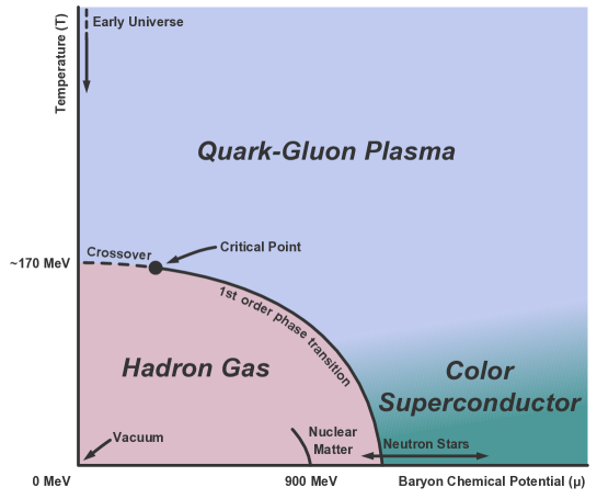
Figure 4: QCD phase diagram.

Basic order parameters for the QCD phase transitions are the Polyakov loop which characterizes the deconfinement transition in the limit of infinitely large quark mass and the chiral condensate for chiral symmetry in the limit of zero quark mass. The expectation value of the Polyakov loop is loosely given by

$$\langle L\rangle\approx\lim_{r\rightarrow\infty}e^{-\beta V(r)}\,,$$

where $V(r)$ is the potential between a static quark-antiquark pair at a distance r, and $\beta\sim 1/T$. The expectation value of the Polyakov loop is zero in confined phase, and it is finite in deconfined phase. While the chiral condensate, which is the simplest order parameter for the chiral symmetry, is non-zero with broken chiral symmetry, vanishing with a restored chiral symmetry. Apart from these order parameters, there are thermodynamic quantities that are relevant to study the QCD phase transition. The equation of state is one of them. The energy density, for instance, has been found to rise rapidly at some critical temperature. This is usually interpreted as deconfinement; liberation of many new degrees of freedom. The fluctuations of conserved charges such as baryon number or electric charge [109, 110] is also an important signal of the quark-hadron phase transition. The quark (or baryon) number susceptibility, which measures the response of QCD to a change of the quark chemical potential is one of such fluctuations [109, 111].

The nature of the chiral transition of QCD depends on the number of quark flavors and the value of the quark mass. For pure $SU(3)$ gauge theory with no quarks, it is first order. In the case of two massless and one massive quarks, the transition is the second order at zero or small quark chemical potentials, and it becomes the first order as we increase the chemical potential. The point where the second order transition becomes the first order is called tricritical point. With physical quark masses of up, down, and strange, the second order at zero or low chemical potential becomes the crossover, and the tricritical point turns into the critical end point.

6.1 Confinement/deconfinement transition

We first discuss the deconfinement transition. In holographic QCD, the confinement to deconfinement phase transition is described by the Hawking-Page transition [112], a phase transition between the Schwarzschild-AdS black hole and thermal AdS backgrounds. This identification was made in [12]. One simple reasoning for this identification is from the observation that the Polyakov expectation value is zero on the thermal AdS geometry, while it is finite on the AdS black hole. See Appendix F for some more description of the Hawking-Page transition and the Polyakov expectation in thermal AdS and AdS black hole. In low-temperature confined phase, thermal AdS, which is nothing but the AdS metric in Euclidean space, dominates the partition function, while at high temperature, AdS-black hole geometry does. This was first discovered in the finite volume boundary case in [12]. In the bottom-up model, it is shown that the same phenomena happen also for infinite boundary volume if there is a finite scale associated with the fifth direction [56].

Here we briefly summarize the Hawking-Page analysis of  [56] done in the hard wall model. The Euclidean gravitational action given by

$$S_{grav}~{}=~{}-\frac{1}{2\kappa^{2}}\int d^{5}x\sqrt{g}\left(\textrm{R}+\frac{12}{L^{2}}\right)\,,$$ (6.1)

where $\kappa^{2}=8\pi G_{5}$ and $L$ is the length scale of the $AdS_{5}$, there are two solutions for the equations of motion derived from the gravitational action. The one is the sliced thermal AdS (tAdS)

$$ds^{2}=\frac{L^{2}}{z^{2}}\left(d\tau^{2}+dz^{2}+d\vec{x}^{2}_{3}\right)\,,$$ (6.2)

where the radial coordinate runs from the boundary of tAdS space $z=0$ to the cut-off $z_{m}$. Here $\tau$ is for the compactified Euclidean time-direction with periodicity $\beta^{\prime}$. The other solution is the AdS black hole (AdSBH) with the horizon $z_{h}$

$$ds^{2}=\frac{L^{2}}{z^{2}}\left(f(z)d\tau^{2}+\frac{dz^{2}}{f(z)}+d\vec{x}^{2}_{3}\right)\,,$$ (6.3)

where $f(z)=1-(z/z_{h})^{4}$. The Hawking temperature of the black hole solution is $T=1/(\pi z_{h})$, which is given by regularizing the metric near the horizon. At the boundary $z=\epsilon$ the periodicity of the time-direction in both backgrounds is the same and so the time periodicity of the tAdS is given by

$$\beta=\pi z_{h}\sqrt{f(\epsilon)}.$$ (6.4)

Now we calculate the action density $V$, which is defined by the action divided by the common volume factor of $R^{3}$. The regularized action density of the tAdS is given by

$$V_{1}(\epsilon)=\frac{4L^{3}}{\kappa^{2}}\int^{\beta^{\prime}}_{0}d\tau\int^{z_{IR}}_{\epsilon}\frac{dz}{z^{5}}\,,$$ (6.5)

and that of the AdSBH is given by

$$V_{2}(\epsilon)=\frac{4L^{3}}{\kappa^{2}}\int^{\pi z_{h}}_{0}d\tau\int^{\bar{z}}_{\epsilon}\frac{dz}{z^{5}}$$ (6.6)

where $\bar{z}={\rm min}(z_{m},z_{h})$. Then, the difference of the regularized actions is given by

$$\Delta V_{g}=\lim_{\epsilon\rightarrow 0}\left[V_{2}(\epsilon)-V_{1}(\epsilon)\right]=\left\{\begin{array}[]{ll}\frac{L^{3}\pi z_{h}}{\kappa^{2}}\frac{1}{2z_{h}^{4}}&z_{m}<z_{h}\\ \\ \frac{L^{3}\pi z_{h}}{\kappa^{2}}\left(\frac{1}{z_{m}^{4}}-\frac{1}{2z_{h}^{4}}\right)&z_{m}>z_{h}.\end{array}\right.$$ (6.7)

When $\Delta V_{g}$ is positive (negative), tAdS (AdSBH) is stable. Thus, at $\Delta V_{g}=0$ there exists a Hawking-Page transition. In the first case $z_{m}<z_{h}$, there is no Hawking-Page transition and the tAdS is always stable. In the second case $z_{m}>z_{h}$, the Hawking-Page transition occurs at

$$T_{c}=2^{1/4}/(\pi z_{m})\,,$$ (6.8)

and at low temperature $T<T_{c}$ (at high temperature $T>T_{c}$) the thermal AdS (the AdS black hole) geometry becomes a dominant background. When we fix the IR cutoff by the $\rho$ meson mass, we obtain $1/z_{m}=323$ MeV and $T_{c}=122$ MeV. In the soft wall model, $T_{c}=191$ MeV [56].

This work has been extended in various directions. The authors of [113] revisited the thermodynamics of the hard wall and soft wall model. They used holographic renormalization to compute the finite actions of the relevant supergravity backgrounds and verify the presence of a Hawking-page type phase transition. They also showed that the entropy, in the gauge theory side, jumps from $N^{0}$ to $N^{2}$ at the transition point [113]. In [114], the extension was done by studying the thermodynamics of AdS black holes with spherical or negative constant curvature horizon, dual to a non-supersymmetric Yang-Mills theory on a sphere or hyperboloid respectively. They also studied charged AdS black holes [115] in the grand canonical ensemble, corresponding to a Yang-Mills theory at finite chemical potential, and found that there is always a gap for the infrared cutoff due to the existence of a minimal horizon for the charged AdS black holes with any horizon topology [114]. With an assumption that the gluon condensate melts out at finite temperature, a Hawking-Page type transition between the dilaton AdS geometry in Eq. (4.4) and the usual AdS black hole has studied in [116].

The effect of the number of quark flavors $N_{f}$ and baryon number density on the critical temperature was investigated by considering a bulk meson action together with the gravity action in [117]. It is shown that the critical temperature decreases with increasing $N_{f}$. As the number density was raised, the critical temperature begins to drop, but it saturates to a constant value even at very large density. This is mostly due to the absence of the back-reaction from number density  [117]. The back-reaction due to the number density has included in [118]. In [119], deconfinement transition of AdS/QCD with $\mathcal{O}({\alpha^{\prime}}^{3})$ corrections were investigated. In [120], thermodynamics of the asymptotically-logarithmically-AdS black-hole solutions of 5D dilaton gravity with a monotonic dilaton potential are analyzed in great detail, where it is shown that in a special case, where the asymptotic geometry in the string frame reduces to flat space with a linear dilaton, the phase transition could be second order. The renormalized Polyakov loop in the deconfined phase of a pure SU(3) gauge theory was computed in [121] based on a soft wall metric model. The result obtained in this work is in good agreement with the one from lattice QCD simulations.

Due to this Hawking-Page transition, we are not to use the black hole in the confined phase, and so we are not to obtain the temperature dependence of any hadronic observables. This is consistent with large $N_{c}$ QCD at leading order. For instance it was shown in [122, 123] that the Wilson loops, both time-like and space-like, and the chiral condensate are independent of the temperature in confining phase to leading order in $1/N_{c}$. This means that the chiral and deconfinement transitions are first order. The deconfinement and chiral phase transitions of an SU(N) gauge theory at large $N_{c}$ were also discussed in [124]. However, in reality we observe temperature dependence of hadronic quantities, and therefore we have to include large $N_{c}$ corrections in holographic QCD in a consistent way. A quick fix-up for this might be to use the temperature dependent chiral condensate as an input in a holographic QCD model and study how this temperature dependence conveys into other hadronic quantities [125].

6.2 Chiral transition

Now we turn to the chiral transition of QCD based on the chiral condensate. In the hard wall model, the chiral symmetry is broken, in a sense, by the IR boundary condition. In case we have a well-defined IR boundary condition at the wall $z=z_{m}$, we could calculate the value of chiral condensate by solving the equation of motion for the bulk scalar $X$. In the case of the AdS black hole we could have a well defined IR boundary condition at the black hole horizon, which allows us to calculate the chiral condensate. For instance in [126], it is shown that with the AdS black hole background the chiral condensate together with the current quark mass is zero both in the hard wall and soft wall models. This is easy to see from the solution of $X_{0}$ in the AdS black hole background [126, 127]

$$X_{0}(z)=z\biggl{(}m_{q}~{}{}_{2}F_{1}(\frac{1}{4},\frac{1}{4},\frac{1}{2},\frac{z^{4}}{z_{h}^{4}})+\sigma_{q}z^{2}~{}{}_{2}F_{1}(\frac{3}{4},\frac{3}{4},\frac{3}{2},\frac{z^{4}}{z_{h}^{4}})\biggr{)}\,.$$ (6.9)

At $z=z_{h}$, both terms in $X_{0}(z)$ diverges logarithmically, which requires to set both of them zero: $m_{q}=0$, $\sigma=0$. This is different from real QCD, where current quark mass can be non-zero in the regime $T>T_{c}$.

The finite temperature phase structure of the Sakai-Sugimoto model was analyzed in [128] to explore deconfinement and chiral symmetry restoration. Depending on a value of the model parameter, it is predicted that deconfinement and chiral symmetry restoration happens at the same temperature or the presence of a deconfined phase with broken chiral symmetry [128]. Phase structure of a stringy D3/D7 model has extensively studied in [129, 130].

6.3 Equation of state and susceptibility

Apart from the chiral condensate, various thermodynamic quantities could serve as an indicator for a transition from hadron to quark-gluon phase. Energy density, entropy, pressure, and susceptibilities are such examples. We first consider energy density and pressure. Schematically, based on the ideal gas picture we discuss how the energy density and pressure tell hadronic matter to quark-gluon plasma. At low temperature thermodynamics of hadron gas will be dominated by pions which are almost massless, while in QGP quarks and gluons are the relevant degrees of freedom. Energy density and pressure of massless pions are

$$\epsilon=\gamma\frac{\pi^{2}}{30}T^{4},~{}~{}~{}p=\gamma\frac{\pi^{2}}{90}T^{4}\,,$$ (6.10)

where the number of degrees of freedom $\gamma$ is three. In the QGP, they are given by

$$\epsilon=\gamma\frac{\pi^{2}}{30}T^{4}+B,~{}~{}~{}p=\gamma\frac{\pi^{2}}{90}T^{4}-B\,,$$ (6.11)

where $\gamma=37$, and $B$ is the bag constant. Apart from the bag constant, the degeneracy factor $\gamma$ changes from $3$ to $37$, and therefore we can expect that the energy density and pressure will increase rapidly at the transition point. Since the dual of the boundary energy-momentum tensor $T_{\mu\nu}$ is the metric, we can obtain the energy density and pressure of a boundary gauge theory from the near-boundary behavior of the gravity solution. To demonstrate how-to, we follow [131, 132]. We first rewrite the gravity solution in the Fefferman-Graham coordinate [133]

$$ds^{2}=\frac{1}{z^{2}}\left(g_{\mu\nu}dx^{\mu}dx^{\nu}-dz^{2}\right)\,.$$ (6.12)

Next, we expand the metric $g_{\mu\nu}$ at the boundary $z\to 0$,

$$g_{\mu\nu}=g_{\mu\nu}^{(0)}+z^{2}g_{\mu\nu}^{(2)}+g_{\mu\nu}^{(4)}+\dots\,.$$ (6.13)

Now we consider flat 4D metric such that $g_{\mu\nu}^{(0)}=\eta_{\mu\nu}$. Then $g_{\mu\nu}^{(2)}=0$ and the vacuum expectation value of the energy momentum tensor is given by

$$\langle T_{\mu\nu}\rangle={\rm const}\cdot g_{\mu\nu}^{(4)}\,.$$ (6.14)

For example, we consider an AdS black hole in the Fefferman-Graham coordinate

$$ds^{2}=\frac{1}{z^{2}}\left(\frac{(1-z^{4}/z_{h}^{4})}{(1+z^{4}/z_{h}^{4})}dt^{2}-(1+z^{4}/z_{h}^{4})d\vec{x}^{2}-dz^{2}\right)\,.$$ (6.15)

Here the temperature is defined by $T=\sqrt{2}/(\pi z_{h})$. Then, we read off

$$\langle T_{\mu\nu}\rangle\approx{\rm diag}(3/z_{h}^{4},1/z_{h}^{4},1/z_{h}^{4},1/z_{h}^{4})\,,$$ (6.16)

which satisfies $\epsilon=3p$. There have been many works on the equations of state for a holographic matter at finite temperature [134]. In [135], the energy density, pressure, and entropy of a deconfined pure Yang-Mills matter were evaluated in the improved holographic QCD model [136]. The energy density and pressure vanish at low temperature, and at the critical temperature, $T_{c}\sim 235$ MeV, they jump up to a finite value, showing the first order phase transition. It is interesting to note that in [137] some high-precision lattice QCD simulations were performed with increasing $N_{c}$ at finite temperature, and the results were compared with those from holographic QCD studies.

Various susceptibilities are also useful quantities to characterize phases of QCD. For instance, the quark number susceptibility has been calculated in holographic QCD in a series of works [126, 138, 139]. The quark number susceptibility was originally proposed as a probe of the QCD chiral phase transition at zero chemical potential [109, 111],

$$\chi_{q}=\frac{\partial n_{q}}{\partial\mu_{q}}.$$ (6.17)

In terms of the retarded Green function $G_{\mu\nu}^{R}(\omega,k)$, the quark number susceptibility can be written as [140],

$$\chi_{q}(T,\mu)=-\lim_{k\to 0}{\mbox{Re}}\Big{(}G_{tt}^{R}(\omega=0,k)\Big{)}.$$ (6.18)

In [138], it is claimed that quark number susceptibility will show a sudden jump at $T_{c}$ in high density regime, and so QCD phase transition in low temperature and high density regime will be always first order. Thermodynamics of a charged dilatonic black hole, which is asymptotically RN-AdS black hole in the UV and AdS${}_{2}\times\mathbf{R}^{3}$ in the IR, including the quark number susceptibility was extensively studied in [141]. The critical end point of the QCD phase diagram was studied in [142] by considering the critical exponents of the specific heat, number density, quark number susceptibility, and the relation between the number density and chemical potential at finite chemical potential and temperature. It is shown that the critical end point located at $T=143$ MeV and $\mu=783$ MeV in the QCD phase diagram [142].

6.4 Dense baryonic matter

Understanding the properties of dense QCD is of key importance for laboratory physics such as heavy ion collision and for our understanding of the physics of stable/unstable nuclei, and of various astrophysical objects such as neutron stars.

To expose an essential physics of dense nuclear matter, we take the Walecka model [143], which describes nuclear matter properties rather well, as an example. The simplest version of the model contains the nucleon $\psi$, omega meson $\omega$, and an isospin singlet, Lorentz scalar meson $\sigma$ whose minimal Lagrangian is

$${\mathcal{L}}=\bar{\psi}(i\not\!\partial+g_{\sigma}\sigma-g_{\omega}\not\!\omega)\psi+\frac{1}{2}(\partial_{\mu}\sigma\partial^{\mu}\sigma-m_{\sigma}^{2}\sigma^{2})-\frac{1}{4}F_{\mu\nu}F^{\mu\nu}+\frac{1}{2}m_{\omega}^{2}\omega_{\mu}\omega_{\mu}\,.$$ (6.19)

Within the mean field approximation, the properties of nuclear matter are mostly determined by the scalar mean field $\bar{\sigma}=(g_{\sigma}/m_{\sigma}^{2})n_{s}$ and the mean field of the time component of the $\omega$ field $\bar{\omega}_{0}=(g_{\omega}/m_{\omega}^{2})n$, where $n$ is the baryon number density and $n_{s}$ is the scalar density. For instance, the pressure of the nuclear matter described by the Walecka is

$$P = \frac{1}{4\pi^{2}}\biggl{[}\frac{2}{3}E_{F}^{*}p_{F}^{3}-{m_{N}^{*}}^{2}E_{F}^{*}p_{F}+{m_{N}^{*}}^{4}\ln(\frac{E_{F}^{*}+p_{F}}{m_{N}^{*}})\biggr{]}$$ (6.21)

$$+\frac{1}{2}\frac{g_{\omega}^{2}}{m_{\omega}^{2}}n^{2}-\frac{1}{2}\frac{g_{\sigma}^{2}}{m_{\sigma}^{2}}n_{s}^{2}\,,$$

where

$$E_{F}^{*}=\sqrt{p_{F}^{2}+{m_{N}^{*}}^{2}},~{}~{}~{}m_{N}^{*}=m_{N}-\frac{g_{\sigma}^{2}}{m_{\sigma}^{2}}n_{s}\,.$$ (6.22)

Further, many successful predictions based on the Walecka model and its generalized versions, Quantum Hadrodynamics, require large scalar and vector fields in nuclei. This implies that to gain a successful description of nuclear matter or nuclei, having both scalar and vector mean fields in the model seem crucial. The importance of the interplay between the scalar and vector fields can be also seen in the static non-relativistic potential between two nucleons. The nucleon-nucleon potential from single $\sigma$-exchange and single $\omega$-exchange is given by

$$V(r)=\frac{g_{\omega}^{2}}{4\pi}\frac{1}{r}e^{-m_{\omega}r}-\frac{g_{\sigma}^{2}}{4\pi}\frac{1}{r}e^{-m_{\sigma}r}\,.$$ (6.23)

Note that single $\sigma$-exchange can be replaced by two pion exchange. If $g_{\omega}>g_{\sigma}$ and $m_{\omega}>m_{\sigma}$, then the potential in Eq. (6.23) captures some essential features of the two nucleon potential to form stable nuclear matter: repulsive at short distance and attraction at intermediate and long distance. We remark here that the scalar field in the Walecka model may not be the scalar associated with a linear realization of usual chiral symmetry breaking in QCD, see for instance [144].

The hard wall model or soft wall model in its original form does not do much in dense matter. This is primarily due to its simple structure and chiral symmetry. Suppose we turn on the time component of a U(1) bulk vector field dual to a boundary number operator, $V_{t}(z)=\mu+\rho z^{2}$. To incorporate this U(1) bulk field into the hard wall mode, we consider U(2) chiral symmetry. The covariant derivative with U(1) vector and axial-vector is given by $D_{\mu}X=\partial_{\mu}X-iA_{L\mu}\,X+iXA_{R\mu}$ and it becomes $D_{\mu}X=\partial_{\mu}X-iX(A_{L\mu}-A_{R\mu})$. Therefore, the U(1) bulk field $V_{\mu}=A_{L\mu}+A_{R\mu}$ does not couple to the scalar $X$, meaning that the physical properties of $X$ are not affected by the chemical potential or number density. Note, however, that the vacuum energy of the hard wall or soft wall model should depend on the chemical potential and number density by the AdS/CFT. One simple way to study the physics of dense matter in the hard or soft wall model is to work with higher dimensional terms in the action. For instance, the role of dimension six terms in the hard wall model was studied in free space [145]. If we turn on the number density through the U(1) bulk field, we have a term like $X_{0}^{2}F_{V}^{2}$, where $F_{V}$ is the field strength of the bulk U(1) gauge field [146]. Then we may see interplay between number density and chiral condensate encoded in $X_{0}$. In [147], based on the hard wall model with the Chern-Simons term it is shown that there exists a Chern-Simons coupling between vector and axial-vector mesons at finite baryon density. This mixes transverse $\rho$ and $a_{1}$ mesons and leads to the condensation of the vector and axial-vector mesons. The role of the scalar density or the scalar field in the hard wall model was explored in [148]. In [149], a back-reaction due to the density is studied in the hard wall model.

Physics of dense matter in Sakai-Sugimoto model has been developed with/without the source term for baryon charge [150]. For instance, in [151] localized and smeared source terms are introduced and a Fermi sea has been observed, though there are no explicit fermionic modes in the model. A deficit with the Sakai-Sugimoto model for nuclear matter might be the absence of the scalar field which is quite important together with U(1) vector field. The phase structure of the D3/D7 model at finite density is studied in [152]. The nucleon-nucleon potential is playing very important role in understanding the properties of nuclear matter. For example, one of the conventional methods to study nuclear matter is to work with the independent-pair approximation, Brueckner’s theory, where two-nucleon potentials are essential inputs. Holographic nuclear forces were studied in [153, 154, 155, 156].

7 Closing remarks

The holographic QCD model has proven to be a successful and promising analytic tool to study non-perturbative nature of low energy QCD. However, its success should always come with “qualitative” since it is capturing only large $N_{c}$ leading physics. To have any transitions from “qualitative” to “quantitative”, we have to invent a way to calculate subleading corrections in a consistent manner. A bit biased, but the most serious defect of the approach based on the gauge/gravity duality might be that it offers inherently macroscopic descriptions of a physical system. For instance, we may understand the QCD confinemnt/deconfinement transition through the Hawking-Page transition, qualitatively. Even though we accept generously the word “qualitatively”, we are not to be satisfied completely since we don’t know how gluons and quarks bound together to form a color singlet hadron or how hadrons dissolve themselves into quark and gluon degrees of freedom. In this sense, the holographic QCD can not be stand-alone. Therefore, the holographic QCD should go together with conventional QCD-based models or theories to guide them qualitatively and to gain microscopic pictures revealed by the conventional approaches.

Finally, we collect some interesting works done in bottom-up models that are not yet properly discussed in this review. Due to our limited knowledge, we could not list all of the interesting works and most results from top-down models will not be quoted. To excuse this defect we refer to recent review articles on holographic QCD  [157].

Deep inelastic scattering has been studied in gauge/gravity duality [158, 159, 160, 161, 162, 163, 164, 165, 166, 167, 168, 169]. Light and heavy mesons were studied in the soft-wall holographic approach [170].

Unusual bound states of quarks are also interesting subjects to work in holographic QCD. In [171], the multi-quark potential was calculated and tetra-quarks were discussed in AdS/QCD. Based on holographic quark-antiquark potential in the static limit, the masses of the states X(3872) or Y(3940) were predicted and also tetra-quark masses with open charm and strangeness were computed in [172]. A hybrid exotic meson, $\pi_{1}$(1400), in [173]. The spectrum of baryons with two heavy quarks was predicted in [174].

Low-energy theorems of QCD and spectral density of the Dirac operator were studied in the soft wall model [175]. A holographic model of hadronization was suggested in [176].

The equation of state for a cold quark matter was calculated in the soft wall metric model with a U(1) gauge field. The result is in agreement with phenomenology [177].

Acknowledgments

We thank Jihun Kim, Yumi Ko, Ik Jae Shin, and Takuya Tsukioka for useful comments on the manuscript. We are slso grateful to Sergey Afonin, Oleg Andreev, Stanley J. Brodsky, Miguel Costa, Guy F. de Teramond, Hilmar Forkel, Jian-Hua Gao, Marco Panero for their comments on the the manuscript. YK expresses his gratitude to Hyun-Chul Kim, Kyung-il Kim, Yumi Ko, Bum-Hoon Lee , Hyun Kyu Lee, Sangmin Lee, Chanyong Park, Ik Jae Shin, Sang-Jin Sin, Takuya Tsukioka, Xiao-Hong Wu, Ulugbek Yakhshiev, Piljin Yi, and Ho-Ung Yee for collaborations in hQCD. We acknowledge the Max Planck Society(MPG), the Korea Ministry of Education, Science and Technology(MEST), Gyeongsangbuk-Do and Pohang City for the support of the Independent Junior Research Group at APCTP.

Appendix A Bulk mass and the conformal dimension of boundary operator

In this Appendix, we summarize the relation between the conformal dimension of a boundary operator and the bulk mass of dual bulk field. We work in the Euclidean version of $AdS_{d+1}$,

$$ds^{2}=\frac{1}{(x^{0})^{2}}\sum_{\mu=0}^{d}(dx^{\mu})^{2}.$$ (A.1)

A.1 Massive scalar case

We first consider a free massive scalar field whose action is given by

$$S=\frac{1}{2}\int d^{d+1}x\sqrt{g}\left(\partial_{\mu}\phi\partial^{\mu}\phi+m^{2}\phi^{2}\right).$$ (A.2)

Let the propagator of $\phi$ be $K(x^{0},\vec{x};\vec{x}^{\prime})$. To solve for $\phi$ in terms of its boundary function $\phi_{0}$, we look for a propagator of $\phi$, a solution $K(x^{0},\vec{x};\vec{x}^{\prime})$ of the Laplace equation on $B_{d+1}$ whose boundary value is a delta function at a point $P$ on the boundary. We take $P$ to be the point at $x_{0}\rightarrow\infty$. The boundary conditions and metric are invariant under translations of the $x_{i}$, then we can consider $K$ as a function of only $x_{0}$, thus $K(x^{0},\vec{x};P)=K(x^{0})$. Then, the equation of motion is

$$\left(-(x^{0})^{d+1}\frac{d}{dx^{0}}(x^{0})^{-d+1}\frac{d}{dx^{0}}+m^{2}\right)K(x^{0})=0\,,$$ (A.3)

where we used

$$\frac{1}{\sqrt{g}}\partial_{\mu}\sqrt{g}\partial^{\mu}=(x^{0})^{d+1}\frac{d}{dx^{0}}(x^{0})^{-d+1}\frac{d}{dx^{0}}.$$ (A.4)

We analyze the equation of motion near the boundary, $x^{0}\rightarrow 0$, and take $K(x^{0})\propto(x^{0})^{\lambda+d}$. From the equation of motion, we have

$$-(\lambda+d)\lambda+m^{2}=0\,,$$ (A.5)

where $\lambda$ is the larger root $\lambda=\lambda_{+}$. The conformal dimension $\Delta$ of the boundary operator is related to the mass m on $AdS_{d+1}$ space by $\Delta=d+\lambda_{+}$. Thus, we obtain

$$(\Delta-d)\Delta=m^{2}\,,$$ (A.6)

or

$$\Delta=\frac{1}{2}\left(d+\sqrt{d^{2}+4m^{2}}\right).$$ (A.7)

A.2 Massive p-form field case

Consider a massive $p$-form potential [178]

$${\cal A}={1\over p!}{\cal A}_{\mu_{1}\ldots\mu_{p}}dx^{\mu_{1}}\cdots dx^{\mu_{p}}\,.$$ (A.8)

The free action of ${\cal A}$ is

$$S={1\over 2}\int_{AdS_{d+1}}\left({\cal F}\wedge{}^{*}{\cal F}+m^{2}{\cal A}\wedge{}^{*}{\cal A}\right),$$ (A.9)

where ${\cal F}=d{\cal A}$ is the field strength $p+1$ form. The variation of this action is

$$\delta S=\int_{AdS_{d+1}}\left(-(-1)^{p}\delta{\cal A}\wedge{}d^{*}{\cal F}+m^{2}\delta{\cal A}\wedge{}^{*}{\cal A}\right)\,,$$

and then the classical equation of motion for ${\cal A}$ from (A.9) is

$$(-1)^{p}d^{*}d{\cal A}-m^{2}\;{}^{*}{\cal A}=0.$$ (A.10)

In addition, ${\cal A}$ satisfies $d^{*}{\cal A}=0$. By using the metric (A.1), the equation of motion (A.10) can be written as

$$\left[(x^{0})^{2}\partial_{\mu}^{2}-(d+1-2p)x^{0}\partial_{0}+(d+1-2p-m^{2})\right]{\cal A}_{0{i_{2}}\ldots{i_{p}}}=0,$$ (A.11)

$$\left[(x^{0})^{2}\partial_{\mu}^{2}-(d-1-2p)x^{0}\partial_{0}-m^{2}\right]{\cal A}_{{i_{1}}\ldots{i_{p}}}$$ (A.12)

$$\hskip 42.67912pt=2x^{0}\left(\partial_{i_{1}}\omega_{0i_{2}\ldots i_{p}}+(-1)^{p-1}\partial_{i_{2}}\omega_{0i_{3}\ldots i_{p}i_{1}}+\cdots\right).$$

Now from the vielbein $e_{a}^{\mu}=x^{0}\delta_{a}^{\mu}$, we introduce fields with flat indices

$$A_{0i_{2}\ldots i_{p}}=(x^{0})^{p-1}{\cal A}_{0i_{2}\ldots i_{p}},\quad A_{i_{1}\ldots i_{p}}=(x^{0})^{p}{\cal A}_{i_{1}\ldots i_{p}}.$$ (A.13)

Then the equations of motion (A.11) of $A_{0i_{2}\ldots i_{p}}$ becomes

$$\left[(x^{0})^{2}\partial_{\mu}^{2}-(d-1)x^{0}\partial_{0}-(m^{2}+p^{2}-pd)\right]A_{0{i_{2}}\ldots{i_{p}}}=0.$$ (A.14)

We consider

$$A_{0i_{2}\ldots i_{p}}\sim(x^{0})^{-\lambda}$$ (A.15)

as $x^{0}\rightarrow 0$. Then substituting this in (A.14) gives

$$0 \!=\! \left[(x^{0})^{2}\partial_{0}^{2}-(d-1)x^{0}\partial_{0}-(m^{2}+p^{2}-pd)\right](x^{0})^{-\lambda}$$

$$\!=\! \left[(x^{0})^{2}\partial_{0}(-\lambda(x^{0})^{-\lambda-1})-(d-1)x^{0}(-\lambda(x^{0})^{-\lambda-1})-(m^{2}+p^{2}-pd)(x^{0})^{-\lambda}\right]$$

$$\!=\! \left[\lambda(\lambda+1)+\lambda(d-1)-(m^{2}+p^{2}-pd)\right](x^{0})^{-\lambda}$$

$$\!=\! \left[\lambda(\lambda+d)-(m^{2}+p^{2}-pd)\right](x^{0})^{-\lambda}$$

and therefore we obtain the relation

$$\lambda(\lambda+d)=m^{2}+p^{2}-pd.$$ (A.16)

With $\Delta=d+\lambda$, we have

$$\quad(\Delta-d)\Delta=m^{2}+p^{2}-pd$$

$$\Rightarrow(\Delta-p)p+(\Delta-p)(\Delta-d)=m^{2}$$

and we finally arrive at

$$(\Delta-d+p)(\Delta-p)=m^{2},$$ (A.17)

or

$$\Delta=\frac{1}{2}\left(d+\sqrt{(d-2p)^{2}+4m^{2}}\right).$$ (A.18)

A.3 General cases

Now for completeness, we list the relations between the conformal dimension $\Delta$ and the mass for the various bulk fields in $AdS_{d+1}$.

1. scalars [3]: $\Delta_{\pm}=\frac{1}{2}(d\pm\sqrt{d^{2}+4m^{2}})$,

2. spinors [179]: $\Delta=\frac{1}{2}(d+2|m|)$,

3. vectors: $\Delta_{\pm}={1\over 2}(d\pm\sqrt{(d-2)^{2}+4m^{2}})$,

4. $p$-forms [178]: $\Delta_{\pm}={1\over 2}(d\pm\sqrt{(d-2p)^{2}+4m^{2}})$,

5. first-order $(d/2)$-forms ($d$ even): $\Delta={1\over 2}(d+2|m|)$,

6. spin-3/2 [181][182]: $\Delta=\frac{1}{2}(d+2|m|)$,

7. massless spin-2 [183]: $\Delta=d$.

Appendix B D3/D7 model and U(1) axial symmetry

In the original AdS/CFT, the duality between type IIB superstring theory on $AdS_{5}\times S^{5}$ and ${\cal N}=4$ super Yang-Mills theory with gauge group $SU(N_{c})$ can be embodied by the low-energy dynamics of a stack of $N_{c}$ D3 branes in Minkowski space. All matter fields in the gauge theory produced by the D3 branes are in the adjoint representation of the gauge group. To introduce the quark degrees of freedom in the fundamental representation, we introduce some other branes in this supersymmetry theory on top of the D3 branes.

B.1 Adding flavour

It was shown in [17] that by introducing $N_{f}$ D7 branes into $AdS_{5}\times S^{5}$, $N_{f}$ dynamical quarks can be added to the gauge theory, breaking the supersymmetry to ${\cal N}=2$. The simplest way to treat D3/D7 system is to work in the limit where the D7 is a probe brane, which means that only a small number of D7 branes are added, while the number of D3 branes $N_{c}$ goes to infinity. In this limit $N_{f}\ll N_{c}$ we may neglect the back-reaction of the D7 branes on $AdS_{5}\times S^{5}$ geometry. In field theory side, this corresponds to ignoring the quark loops, quenching the gauge theory.

	0	1	2	3	4	5	6	7	8	9
D3	$\circ$	$\circ$	$\circ$	$\circ$
D7	$\circ$	$\circ$	$\circ$	$\circ$	$\circ$	$\circ$	$\circ$	$\circ$

Table 3: The D3/D7-brane intersection in $9+1$ dimensional flat space.

The D7 branes are added in such a way that they extend parallel in Minkowski space and extend in spacetime as given in Table 3. The massless modes of open strings both ends on the $N_{c}$ D3 branes give rise to ${\cal N}=4$ degrees of freedom of supergravity on $AdS_{5}\times S^{5}$ consisting of the $SU(N_{c})$ vector bosons, four fermions and six scalars. In the limit of large $N_{c}$ at fixed but large ’t Hooft coupling $\lambda=g_{YM}^{2}N_{c}=g_{s}N_{c}\gg 1$ , the D3 branes can be replace with near horizon geometry that is given by

$$ds^{2} =\frac{r^{2}}{R^{2}}(-dt^{2}+dx_{1}^{2}+dx_{2}^{2}+dx_{3}^{2})+\frac{R^{2}}{r^{2}}d\vec{y}^{2}$$

$$=\frac{r^{2}}{R^{2}}(-dt^{2}+dx_{1}^{2}+dx_{2}^{2}+dx_{3}^{2})+\frac{R^{2}}{r^{2}}\left(d\rho^{2}+\rho^{2}d\Omega_{3}^{2}+dy_{5}^{2}+dy_{6}^{2}\right)$$ (B.1)

where $\vec{y}=(y_{1},\ldots,y_{6})$ parameterize the 456789 space and $r^{2}\equiv\vec{y}^{2}$. $R$ is the radius of curvature $R^{2}=\sqrt{4\pi g_{s}N_{c}}\alpha^{\prime}$ and $d\Omega_{3}^{2}$ is the three-sphere metric. The dynamics of the probe D7 brane is described by the combined DBI and Chern-Simons actions [5, 184],

$$S_{D7}=-T_{7}\int d^{8}x\sqrt{-{\rm det}\left(P[g]_{ab}+2\pi\alpha^{\prime}F_{ab}\right)}+\frac{(2\pi\alpha^{\prime})^{2}}{2}T_{7}\int P[C^{(4)}]\wedge F\wedge F\,.$$ (B.2)

where $g$ is the bulk metric (B.1) and $C^{(4)}$ is the four form potential. $T_{7}=1/((2\pi)^{7}g_{s}\alpha^{\prime}4)$ is the D7 brane tension and $P$ denotes the pullback. $F_{ab}$ is the world-volume field strength.

The addition of D7 branes to this system as in Table 3 breaks the supersymmetry to ${\cal N}=2$. The lightest modes of the 3-7 and 7-3 open strings corresponds the quark supermultiplets in the field theory. If the D7 brane and the D3 brane overlap then SO(6) symmetry is broken into $SO(4)\times SO(2)\sim SO(2)_{R}\times SO(2)_{L}\times U(1)_{R}$ in the transverse directions to D3 and so preserves 1/4 of the supersymmetry. The $SO(4)$ rotates in 4567, while the $SO(2)$ group acts on 89 in 3. The induced metric on D7 takes the form, in general, as

$$ds_{D7}^{2}=\frac{r^{2}}{R^{2}}\eta_{\mu\nu}dx^{\mu}dx^{\nu}+\frac{R^{2}}{r^{2}}\left((1+y_{5}^{\prime 2}+y_{6}^{\prime 2})d\rho^{2}+\rho^{2}d\Omega_{3}^{2}\right)$$ (B.3)

where $y_{5}^{\prime}=dy_{5}/d\rho$ and $y_{6}^{\prime}=dy_{6}/d\rho$. When the D7 brane and the D3 brane overlap, the embedding is

$$y_{5}=0,\qquad y_{6}=0$$ (B.4)

and the induced metric on the D7 brane is replaced by

$$ds_{D7}^{2}=\frac{\rho^{2}}{R^{2}}\eta_{\mu\nu}dx^{\mu}dx^{\nu}+\frac{R^{2}}{\rho^{2}}\left(d\rho^{2}+\rho^{2}d\Omega_{3}^{2}\right)\,.$$ (B.5)

The D7 brane fills $AdS_{5}$ and is wrapping a three sphere of $S^{5}$. In this case the quarks are massless and the R-symmetry of the theory is $SU(2)_{R}\times U(1)_{R}$ and we have an extra $U(1)_{R}$ chiral symmetry.

If the D7 brane is separated from the D3 branes in the 89-plane direction by distance $L$, then the minimum length string has non-zero energy and the quark gains a finite mass, $m_{q}=L/2\pi\alpha^{\prime}$. It is known that the R-symmetry is then only $SU(2)_{R}$ and separation of D7 and D3 breaks the $SO(2)\sim U(1)_{R}$ that acts on the 89-plane. In this case, we can set for the embedding as

$$y_{5}=0,\qquad y_{6}=y_{6}(\rho)\,.$$ (B.6)

Then, the action for a static D7 embedding (with $F_{ab}$ zero on its world volume) becomes

$$S_{D7} =-T_{7}\int d^{8}x\sqrt{-{\rm det}\left(P[g]_{ab}\right)}=-T_{7}\int d^{8}x\sqrt{-{\rm det}g_{ab}}\sqrt{1+g^{ab}\partial_{a}y_{i}\partial_{b}y_{j}g_{ij}}$$

$$=-T_{7}\int d^{8}x\epsilon_{3}\rho^{3}\sqrt{1+(\partial_{\rho}y_{5})^{2}+(\partial_{\rho}y_{6})^{2}}\,,$$ (B.7)

where $i,j=5,6$ and $\epsilon_{3}$ is the determinant from the three sphere. The ground state configuration of the D7 brane is given by the equation of motion with $y_{5}=0$

$$\frac{d}{d\rho}\left[\frac{\rho^{3}\partial_{\rho}y_{6}}{\sqrt{1+(\partial_{\rho}y_{6})^{2}}}\right]=0\,.$$ (B.8)

The solution of this equation has an asymptotic behavior at UV ($\rho\rightarrow\infty$) as

$$y_{6}\simeq m+\frac{c}{\rho^{2}}+\ldots\,.$$ (B.9)

Now we can identify [158] that $m$ corresponds to the quark mass and $c$ is for the quark condensate $\langle\bar{\psi}\psi\rangle$ in agreement with the AdS/CFT dictionary.

B.2 Chiral symmetry breaking

One of the significant feature of QCD is chiral symmetry breaking by a quark condensate $\bar{\psi}\psi$. The $U(1)$ symmetry under which $\psi$ and $\bar{\psi}$ transform as $\psi\rightarrow e^{-i\alpha}\psi$, $\bar{\psi}\rightarrow e^{i\alpha}\bar{\psi}$ in the gauge theory corresponds to a $U(1)$ isometry in the $y_{5}y_{6}$ plane transverse to the D7 brane. This $U(1)$ symmetry can be explicitly broken by a non-vanishing quark mass due to the separation of the D7 brane from the stack of D3 branes in the $y_{5}+iy_{6}$ direction. Assume the embedding as $y_{5}=0$ and $y_{6}\sim c/\rho^{2}$, then by a small rotation $e^{-i\epsilon}$ on $y_{5}+iy_{6}$ generates $y_{5}^{\prime}\simeq\epsilon c/\rho^{2}$ and $y_{6}^{\prime}\simeq y_{6}$ up to the ${\cal O}(\epsilon^{2})$ order.

In [18] the embedding of a D7 probe brane is embodied in the Constable-Myers background and the regular solution $y_{6}\sim m+c/\rho^{2}$ of the embedding $y_{5}=0$, $y_{6}=y_{6}(\rho)$ shows the behavior $c\neq 0$ as $m\rightarrow 0$ which corresponds to the spontaneous chiral symmetry breaking by a quark condensate. In [185], the chiral symmetry breaking comes from a cosmological constant with a constant dilaton configuration which is dual to the ${\cal N}=4$ gauge theory in a four-dimensional AdS space.

B.3 Meson mass spectrum

The open string modes with both ends on the flavour D7 branes are in the adjoint of the $U(N_{f})$ flavour symmetry of the quarks and hence can be interpreted as the mesonic degrees of freedom. As an example, we discuss the fluctuation modes for the scalar fields (with spin 0) following the argument of [186]. The directions transverse to the D7 branes are chosen to be $y_{5}$ and $y_{6}$ and the embedding is

$$y_{5}=0+\chi,\qquad y_{6}=L+\varphi$$ (B.10)

where $\delta y_{5}=\chi$ and $\delta y_{6}=\varphi$ are the scalar fluctuations of the transverse direction. To calculate the spectra of the world-volume fields it is sufficient to work to quadratic order. For the scalars, we can write the relevant Lagrangian density as

$${\cal L}_{D7} =-T_{7}\sqrt{-{\rm det}P[g]_{ab}}$$

$$=-T_{7}\sqrt{-{\rm det}g_{ab}}\sqrt{1+g^{ab}\left(\partial_{a}\chi\partial_{b}\chi g_{55}+\partial_{a}\varphi\partial_{b}\varphi g_{66}\right)}$$

$$=-T_{7}\sqrt{-{\rm det}g_{ab}}\sqrt{1+g^{ab}\frac{R^{2}}{r^{2}}\left(\partial_{a}\chi\partial_{b}\chi+\partial_{a}\varphi\partial_{b}\varphi\right)}$$

$$\simeq-T_{7}\sqrt{-{\rm det}g_{ab}}\left(1+\frac{1}{2}\frac{R^{2}}{r^{2}}{g^{ab}}\left(\partial_{a}\chi\partial_{b}\chi+\partial_{a}\varphi\partial_{b}\varphi\right)\right)$$ (B.11)

where $P[g]_{ab}$ is the induced metric on the D7 world-volume. In spherical coordinates with $r^{2}=\rho^{2}+L^{2}$, this can be written as

$${\cal L}_{D7}\simeq-T_{7}\rho^{3}\epsilon_{3}\left(1+\frac{1}{2}\frac{R^{2}}{\rho^{2}+L^{2}}{g^{ab}}\left(\partial_{a}\chi\partial_{b}\chi+\partial_{a}\varphi\partial_{b}\varphi\right)\right)$$ (B.12)

where $\epsilon_{3}$ is the determinant of the metric on the three sphere. Then the equations of motion becomes

$$\partial_{a}\left(\frac{\rho^{3}\epsilon_{3}}{\rho^{2}+L^{2}}g^{ab}\partial_{b}\Phi\right)=0\,,$$ (B.13)

where $\Phi$ is used to denote the real fluctuation either $\chi$ or $\varphi$. Evaluating a bit more, we have

$$\frac{R^{4}}{(\rho^{2}+L^{2})^{2}}\partial_{\mu}\partial^{\mu}\Phi+\frac{1}{\rho^{3}}\partial_{\rho}(\rho^{3}\partial_{\rho}\Phi)+\frac{1}{\rho^{2}}\nabla_{i}\nabla^{i}\Phi=0\ ,$$ (B.14)

where $\nabla_{i}$ is the covariant derivative on the three-sphere. We apply the separation of variables to write the modes as

$$\Phi=\phi(\rho)e^{ik\cdot x}{\cal Y}^{\ell}(S^{3})\ ,$$ (B.15)

where ${\cal Y}^{\ell}(S^{3})$ are the scalar spherical harmonics on $S^{3}$, which transform in the $(\ell/2,\ell/2)$ representation of $SO(4)$ and satisfy

$$\nabla^{i}\nabla_{i}{\cal Y}^{\ell}=-\ell(\ell+2){\cal Y}^{\ell}\ .$$ (B.16)

The meson mass is defined by

$$M^{2}\equiv-k^{2}\,.$$ (B.17)

Now we define $\varrho=\rho/L$ and $\bar{M}^{2}=-k^{2}R^{4}/L^{2}$, and then the equation for $\phi(\rho)$ is

$$\partial_{\varrho}^{2}\phi+\frac{3}{\varrho}\partial_{\varrho}\phi+\left(\frac{\bar{M}^{2}}{(1+\varrho^{2})^{2}}-\frac{\ell(\ell+2)}{\varrho^{2}}\right)\phi=0\ .$$ (B.18)

This equation was solved in [186] in terms of the hypergeometric function. To solve the equation, we first set

$$\phi(\varrho)=\varrho^{\ell}(1+\varrho^{2})^{-\alpha}P(\varrho),$$ (B.19)

where

$$2\alpha=-1+\sqrt{1+\bar{M}^{2}}\geq 0\,.$$ (B.20)

With a new variable $y=-\varrho^{2}$, (B.18) becomes

$$y(1-y)P^{\prime\prime}(y)+[c-(a+b+1)y]P^{\prime}(y)-abP(y)=0$$ (B.21)

where $a=-\alpha$, $b=-\alpha+\ell+1$ and $c=\ell+2$. The general solution is taken by $\alpha\geq 0$ and by noting that the scalar fluctuations are real for $-\infty<y\leq 0$, one finds, up to a normalization constant, the solution of $\phi$

$$\phi(\rho)=\frac{\rho^{\ell}}{(\rho^{2}+L^{2})^{\alpha}}F\left(-\alpha,\ -\alpha+\ell+1;\ \ell+2\ ;\ -\rho^{2}/L^{2}\right).$$ (B.22)

Imposing the nomalizability at $\rho\to\infty$, we obtain

$$-\alpha+\ell+1=-n,\qquad n=0,1,2,\ldots\,.$$ (B.23)

The solution is then

$$\phi(\rho)=\frac{\rho^{\ell}}{(\rho^{2}+L^{2})^{n+\ell+1}}\ F\left(-(n+\ell+1)\ ,\ -n\ ;\ \ell+2\ ;\ -\rho^{2}/L^{2}\right)\$$ (B.24)

and from the condition (B.23) we get

$$\bar{M}^{2}=4(n+\ell+1)(n+\ell+2)\ .$$ (B.25)

Then by the definition of meson mass (B.17), we derive the four-dimensional mass spectrum of the scalar meson

$$M_{s}(n,\ell)=\frac{2L}{R^{2}}\sqrt{(n+\ell+1)(n+\ell+2)}\ .$$ (B.26)

B.4 Mesons at finite temperature

In previous sections, we have focused on gauge theories and their gravity dual at zero temperature. To understand the thermal properties of gauge theories using the holography, we work with the AdS-Schwarzschild black hole which is dual to ${\cal N}=4$ gauge theory is at finite temperature [3, 12]. The Euclidean AdS-Schwarzschild solution is given by

$$ds^{2}=\frac{K(r)}{R^{2}}d\tau^{2}+R^{2}{\frac{dr^{2}}{K(r)}}+\frac{r^{2}}{R^{2}}d\vec{x}^{2}+R^{2}d\Omega_{5}^{2}\,,$$ (B.27)

where

$$K(r)=r^{2}\left(1-{\frac{r_{H}^{4}}{r^{4}}}\right)\,.$$ (B.28)

For $r\gg r_{H}$, this approaches $AdS_{5}\times S^{5}$ and the AdS radius $R$ is related to the ’t Hooft coupling by $R^{2}=\sqrt{4\pi\lambda}\alpha^{\prime}$. Note that the $S^{1}$ parameterized by $\tau$ collapses at $r=r_{H}$, which is responsible for the existence of an area law of the Wilson loop and a mass gap in the dual field theory. This geometry is smooth and complete if the imaginary time $\tau$ is periodic with the period $\beta=R^{2}\pi/r_{H}$. The temperature of the field theory corresponds to the Hawking temperature is given by $T=1/\beta=r_{H}/(R^{2}\pi)$. At finite temperature, the fermions have anti-periodic boundary conditions in $\tau$ direction [12] and the supersymmetry is broken. In addition, the adjoint scalars also become massive at one loop. Thus, fermions and scalars decouple.

We now introduce D7 branes in this background. It is convenient to change the variable in the metric (B.27) such that the it possesses an explicit flat 6-plane. To this end, we change the variable from $r$ to $w$ as

$$\frac{dr^{2}}{K(r)}=\frac{r^{2}dr^{2}}{r^{4}-r_{H}^{4}}\equiv\frac{dw^{2}}{w^{2}}\,,$$ (B.29)

and take $R\equiv 1$. One of the solutions is

$$2w^{2}=r^{2}+\sqrt{r^{4}-r_{H}^{4}}\quad\textrm{ or }\quad r^{2}=\frac{w^{4}+w_{H}^{4}}{w^{2}}$$ (B.30)

and $w_{H}=r_{H}/\sqrt{2}$. Then the metric (B.27) becomes

$$ds^{2} =\frac{(w^{4}-w_{H}^{4})^{2}}{w^{2}(w^{4}+w_{H}^{4})}dt^{2}+\left(w^{2}+\frac{w_{H}^{4}}{w^{2}}\right)d\vec{x}^{2}+\frac{1}{w^{2}}(dw^{2}+w^{2}d\Omega_{5}^{2})$$

$$=\frac{(w^{4}-w_{H}^{4})^{2}}{w^{2}(w^{4}+w_{H}^{4})}dt^{2}+\left(w^{2}+\frac{w_{H}^{4}}{w^{2}}\right)d\vec{x}^{2}+\frac{1}{w^{2}}(d\rho^{2}+\rho^{2}d\Omega_{3}^{2}+dw_{5}^{2}+dw_{6}^{2})\,,$$ (B.31)

where $d\Omega_{3}^{2}$ is the three-sphere metric. The D7 brane is embedded in the static gauge, which worldvolume coordinates are now identified with $x_{0,1,2,3}$ and $w_{1,2,3,4}$ and the transverse fluctuations will be parameterized by $w_{5}$ and $w_{6}$. The radial coordinate is given by

$$w^{2}=\sum_{i=1}^{6}w_{i}^{2}=\rho^{2}+w_{5}^{2}+w_{6}^{2}.$$ (B.32)

At large $w$, this geometry asymptotically approaches $AdS_{5}\times S^{5}$ and the D7 embedding should approach the constant solutions $w_{5}=0,w_{6}=const$ which is the same as the exact solution in section B.1. To consider the deformation, we take the following ansatz for the embedding

$$w_{5}=0,\qquad w_{6}=w_{6}(\rho)$$ (B.33)

Then, the action of D7 becomes

$$S_{D7} =-T_{7}\int d^{8}x\sqrt{-{\rm det}P[g]_{ab}}=-T_{7}\int d^{8}x\sqrt{-{\rm det}g_{ab}}\sqrt{1+g^{ab}\left(\partial_{a}w_{5}\partial_{b}w_{5}g_{55}+\partial_{a}w_{6}\partial_{b}w_{6}g_{66}\right)}$$

$$=-T_{7}\int d^{8}x~{}\epsilon_{3}~{}{\cal G}(\rho,w_{5},w_{6})\sqrt{1+(\partial_{\rho}w_{5})^{2}+(\partial_{\rho}w_{6})^{2}}\,,$$ (B.34)

where $\epsilon_{3}$ is the determinant of the three-sphere metric and the function ${\cal G}(\rho,w_{5},w_{6})$ is given by

$${\cal G}(\rho,w_{5},w_{6})=\sqrt{\frac{(w^{4}-w_{H}^{4})^{2}(w^{4}+w_{H}^{4})^{2}\rho^{6}}{w^{16}}}=\rho^{3}\left(1-\frac{w_{H}^{8}}{(\rho^{2}+w_{5}^{2}+w_{6}^{2})^{4}}\right).$$ (B.35)

With the assumption $w_{5}=0$, the equation of motion takes the form

$$\frac{d}{d\rho}\left[\rho^{3}\left(1-\frac{w_{H}^{8}}{(\rho^{2}+w_{6}^{2})^{4}}\right)\frac{\partial_{\rho}w_{6}}{\sqrt{1+(\partial_{\rho}w_{6})^{2}}}\right]-\frac{8w_{H}^{8}\rho^{3}w_{6}}{(\rho^{2}+w_{6}^{2})^{5}}\sqrt{1+(\partial_{\rho}w_{6})^{2}}=0\,.$$ (B.36)

With the solution of this equation, the induced metric on the D7 brane is given by

$$ds_{D7}^{2}=\frac{(\tilde{w}^{4}-w_{H}^{4})^{2}}{\tilde{w}^{2}(\tilde{w}^{4}+w_{H}^{4})}dt^{2}+\left(\tilde{w}^{2}+\frac{w_{H}^{4}}{\tilde{w}^{2}}\right)d\vec{x}^{2}+\frac{1+(\partial_{\rho}w_{6})^{2}}{\tilde{w}^{2}}d\rho^{2}+\frac{\rho^{2}}{\tilde{w}^{2}}d\Omega_{3}^{2}\,,$$ (B.37)

with $\tilde{w}^{2}=\rho^{2}+w_{6}^{2}(\rho)$ and the D7-brane metric becomes $AdS_{5}\times S^{3}$ for $\rho\gg w_{H},w_{6}$.

The asymptotic solution at large $\rho$ is of the form

$$w_{6}(\rho)\sim m+\frac{c}{\rho^{2}}\,.$$ (B.38)

As discussed in section B.1, the parameters $m$ and $c$ are interpreted as a quark mass and bilinear quark condensate $\langle\bar{\psi}\psi\rangle$, respectively. With suitable boundary conditions for the second order equation (B.36), one can solve it numerically by the shooting method. The results are shown in Figure 5.

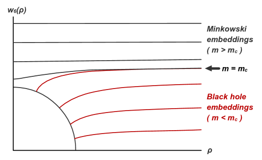
Figure 5: Two classes of regular solutions in the AdS black hole background.

We see that there can be two different classifications for the D7 brane embeddings. First, for large quark masses the D7 brane ends outside the horizon. It can be interpreted that the D7 brane tension is stronger than the attractive force of the black hole. Such a D7 brane solution is called a Minkowski embedding. They behave similarly to the supersymmetric solutions in $AdS_{5}\times S^{5}$. Second, for small masses the D7 brane ends at the horizon $w=w_{H}$ at which the $S^{1}$ of the black hole geometry collapses. This is called a black hole embedding. These two classes of embeddings also differ by their topology. The D7 brane topology is $R^{3}\times B^{4}\times S^{1}$ for Minkowski embedding and $R^{3}\times S^{3}\times B^{2}$ for black hole embedding. The change in the topology is related to a phase transition in the dual field theory.

Appendix C D4/D8/$\overline{\rm D8}$ model and non-Abelian chiral symmetry

The D3/D7 system is a supersymmetric configuration which gives gauge theories in the ultra-violet and only has a $U(1)_{A}$ symmetry. To realize more realistic non-Abelian chiral symmetry, Sakai and Sugimoto proposed D4/D8/$\overline{\rm D8}$ brane configuration [21, 22] which is intrinsically non-supersymmetric. They placed probe D8 and $\overline{\rm D8}$ branes into the $N_{c}$ D4 background of the fundamental representation of the $SU(N_{c})$ gauge group. The D4/D8/$\overline{\rm D8}$ intersection in 9+1 dimensional flat space is given in Table 4.

	0	1	2	3	(4)	5	6	7	8	9
D4	$\circ$	$\circ$	$\circ$	$\circ$	$\circ$
D8-$\overline{\rm D8}$	$\circ$	$\circ$	$\circ$	$\circ$		$\circ$	$\circ$	$\circ$	$\circ$	$\circ$

Table 4: The D4/D8/$\overline{\rm D8}$ brane intersection in $9+1$ dimensional flat space.

In this configuration, $N_{c}$ D4-branes are compactified on a direction ($x^{4}$) wrapped on $S^{1}$. We impose anti-periodic boundary conditions on this $S^{1}$ in order to break the supersymmetry. $N_{f}$ D8 and $\overline{\rm D8}$ pairs are put in the transverse to the $S^{1}$. Then, from the D4-D8 and D4-$\overline{\rm D8}$ open strings we obtain $N_{f}$ flavors of massless chiral and anti-chiral quark fields of the $U(N_{c})$ gauge group. If we take the strong coupling limit to take the large $N_{c}$ dual, the D8 and $\overline{\rm D8}$ will overlap into a single curved D8 brane, which is interpreted as non-Abelian chiral symmetry breaking. The $U(N_{f})_{D8}\times U(N_{f})_{\overline{D8}}$ gauge symmetry of the D8 and $\overline{\rm D8}$ branes is interpreted as the $U(N_{f})_{L}\times U(N_{f})_{R}$ chiral symmetry. These configurations are sketched in Figure 6.

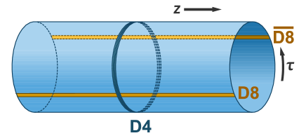
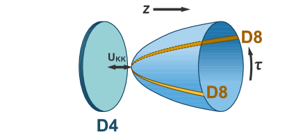
Figure 6: Sketch of the D4/D8/$\overline{\rm D8}$ configuration.

C.1 Background D4 and probe D8 branes

In order to obtain a holographic dual of the the large $N_{c}$ gauge theory with non-Abelian chiral symmetry, we consider the SUGRA description of the D4/D8/$\overline{\rm D8}$ system as discussed above. Assuming $N_{f}\ll N_{c}$, we treat D8-$\overline{\rm D8}$ pairs as probe D8 branes embedded in the D4 background. By taking the near horizon limit of the geometry of $N_{c}$ stack of D4 branes wrapped on a circle, we obtain the D4 brane solution geometry

$$ds^{2}=\left(\frac{U}{R}\right)^{3/2}\left(\eta_{\mu\nu}dx^{\mu}dx^{\nu}+f(U)d\tau^{2}\right)+\left(\frac{R}{U}\right)^{3/2}\left(\frac{dU^{2}}{f(U)}+U^{2}d\Omega_{4}^{2}\right)$$ (C.1)

with $f(U)\equiv 1-U_{KK}^{3}/U^{3}$. Here $x^{\mu}$ ($\mu=0,1,2,3$) and $\tau$ are the directions along which the D4-brane is extended and $R$ is the radius of curvature related to the string coupling $g_{s}$ and string length $l_{s}$ as $R^{3}=\pi g_{s}N_{c}l_{s}^{3}$. There is a nonzero four-form flux $F_{4}=dC_{3}=2\pi N_{c}\epsilon_{4}/V_{4}$ with the volume form $\epsilon_{4}$ and a dilaton $e^{-\phi}=g_{s}\left(U/R\right)^{-3/4}$. $U$ is the holographic direction and bounded from below by the condition $U\geq U_{KK}$. As $U\rightarrow U_{KK}$ the radius of $S^{1}$ parameterized by $\tau$ shrinks into zero and then the D8 and $\overline{\rm D8}$ branes are connected at some point $U=U_{0}$. In this case the gauge symmetry is $U(N_{f})$. The configuration is then interpreted as a theory with massless quarks with chiral symmetry breaking, which is sketched on the right hand side of Figure 6. In order to avoid a singularity at $U=U_{KK}$, $\tau$ must be periodic with period $\delta\tau\equiv=4\pi R^{3/2}/3U_{KK}^{1/2}$, which defines the Kaluza-Klein mass, $M_{KK}=2\pi/\delta\tau=3U_{KK}^{1/2}/2R^{3/2}$.

Next, we consider the induced metric on the D8 probe brane in the D4 background with an ansatz $U=U(\tau)$. Then, $dU^{2}=(dU/d\tau)^{2}\tau^{2}=U^{\prime}(\tau)^{2}d\tau^{2}$ and the induced metric is given by

$$ds^{2}_{D8}=\left(\frac{U}{R}\right)^{3/2}\eta_{\mu\nu}dx^{\mu}dx^{\nu}+\left(\left(\frac{U}{R}\right)^{3/2}f(U)+\left(\frac{R}{U}\right)^{3/2}\frac{U^{\prime 2}}{f(U)}\right)d\tau^{2}+\left(\frac{R}{U}\right)^{3/2}U^{2}d\Omega_{4}^{2}\,,$$ (C.2)

The D8 brane DBI action now becomes

$$S_{D8}\sim\int d^{4}xd\tau\epsilon_{4}e^{-\phi}\sqrt{-{\rm det}(g_{D8})}\sim\int d^{4}xd\tau U^{4}\sqrt{f(U)+\left(\frac{R}{U}\right)^{3}\frac{U^{\prime 2}}{f(U)}}$$ (C.3)

Since the integrand of (C.3) does not explicitly depend on $\tau$, we obtain the energy conservation

$$\frac{d}{d\tau}\left(\frac{\partial{\cal L}}{\partial U^{\prime}}\partial U^{\prime}-{\cal L}\right)=\frac{d}{d\tau}\left(\frac{U^{4}f(U)}{f(U)+R^{3}U^{\prime 2}/U^{3}f(U)}\right)=0.$$ (C.4)

Let $U(0)=U_{0}$ and assume $U^{\prime}(0)=0$ at $\tau=0$, then the solution of (C.4) will be

$$\tau(U)=U_{0}^{4}f(U_{0})^{1/2}\int_{U_{0}}^{U}\frac{dU}{(U/R)^{3/2}f(U)\sqrt{U^{8}f(U)-U_{0}^{8}f(U_{0})}}.$$ (C.5)

It can be shown that $\tau(U\rightarrow\infty)$ is a monotonically decreasing function of $U_{0}$, roughly $\tau(\infty)\sim U_{0}^{-9/2}$, that is varying from $\tau(\infty)|_{U=U_{KK}}=\delta/4$ to $\tau(\infty)|_{U\rightarrow\infty}=0$. In the limit $U_{0}=U_{KK}$, the D8 and $\overline{\rm D8}$ branes are at antipodal points on the $S^{1}$ parameterized by $\tau$. And when $U_{0}\rightarrow\infty$, the D8 and $\overline{\rm D8}$ separate far away from each other. Here we concentrate on the case $U_{0}=U_{KK}$. For the sake of convenience, we perform the change of variables

$$U^{3}=U_{KK}^{3}+U_{KK}r^{2},\qquad\theta=\frac{2\pi}{\delta\tau}\tau=\frac{3U_{KK}^{1/2}}{2R^{3/2}}\tau\,.$$ (C.6)

Now, the induced metric (C.2) on a D8 brane becomes

$$ds^{2}_{D8}=\left(\frac{U}{R}\right)^{3/2}\eta_{\mu\nu}dx^{\mu}dx^{\nu}+\frac{4}{9}\left(\frac{U}{R}\right)^{3/2}\left(\frac{U_{KK}}{U}dr^{2}+r^{2}d\theta\right)+\left(\frac{R}{U}\right)^{3/2}U^{2}d\Omega_{4}^{2}.$$ (C.7)

We change the variables once more as

$$y=r\cos\theta,\qquad z=r\sin\theta\,,$$ (C.8)

accordingly, the $dr$ and $d\theta$ part of (C.7) read

$$\frac{U_{KK}}{U}dr^{2}+r^{2}d\theta=(1-h(r)z^{2})dz^{2}+(1-h(r)y^{2})dy^{2}-2h(r)zydzdy$$ (C.9)

with $h(r)=1/r^{2}(1-U_{KK}/U)$. Near $U=U_{KK}$, (C.7) approaches a flat two-dimensional plane and $h(r)$ is a regular function in the neighborhood of $r=0$. Then, $y(x^{\mu},z)=0$ can be a solution of the equation of motion of the probe D8 brane’s world-volume theory and the stability of the solution can be shown by examination of small fluctuations around it [21]. Thus, from (C.6) we have

$$U^{3}=U_{KK}^{3}+U_{KK}z^{2}$$ (C.10)

and the induced metric on the D8 brane

$$ds^{2}_{D8}=\left(\frac{U}{R}\right)^{3/2}\eta_{\mu\nu}dx^{\mu}dx^{\nu}+\frac{4}{9}\left(\frac{U}{R}\right)^{3/2}\frac{U_{KK}}{U}dz^{2}+\left(\frac{R}{U}\right)^{3/2}U^{2}d\Omega_{4}^{2}.$$ (C.11)

C.2 Gauge field and meson spectrum

Now, we consider the gauge field on the probe D8 brane configuration. The gauge field on the D8 brane $A_{M}$ ($M=0,1,2,3,5,6,7,8,z$) has nine components, and among them we are interested in the $SO(5)$ singlet states, so we can set $A_{\alpha}=0$ for $\alpha=5,6,7,8$. We assume that $A_{\mu}$ and $A_{z}$ are independent of the coordinates on the $S^{4}$. Then the DBI action for $D8$ branes becomes

$$S_{D8} =-T_{8}\int d^{9}x\sqrt{-{\rm det}\left(g_{ab}+2\pi\alpha^{\prime}F_{ab}\right)}+S_{CS}$$

$$=-\tilde{T}(2\pi\alpha^{\prime})^{2}\int d^{4}xdz\left[\frac{R^{3}}{4U}\eta^{\mu\nu}\eta^{\rho\sigma}F_{\mu\nu}F_{\rho\sigma}+\frac{9}{8}\frac{U^{3}}{U_{KK}}\eta^{\mu\nu}F_{\mu z}F_{\nu z}\right]+{\cal O}(F^{3})\,,$$ (C.12)

where $\tilde{T}=(2/3)R^{3/2}U_{KK}^{1/2}T_{8}V_{4}g_{s}^{-1}$. We expand the gauge fields $A_{\mu}$ and $A_{z}$ in terms of the complete sets of the Kaluza-Klein (KK) modes profile functions $\{\psi_{n}(z)\}$ and $\{\phi_{n}(z)\}$, respectively,

$$A_{\mu}(x,z) =\sum_{n\geq 0}v_{\nu}^{(n)}(x)\psi_{n}(z),$$ (C.13)

$$A_{z}(x,z) =\sum_{n\geq 0}\varphi^{(n)}(x)\phi_{n}(z).$$ (C.14)

and consequently, the field strengths read

$$F_{\mu\nu}(x,z) =\sum_{n\geq 0}\left(\partial_{\mu}v_{\nu}^{(n)}(x)\psi_{n}(z)\right)\equiv\sum_{n\geq 0}F_{\mu\nu}^{(n)}(x)\psi_{n}(z),$$ (C.15)

$$F_{\mu z}(x,z) =\sum_{n\geq 0}\left(\partial_{\mu}\varphi^{(n)}(x)\phi_{n}(z)-v_{\mu}^{(n)}(x)\partial_{z}\psi_{n}(z)\right).$$ (C.16)

Then, the action (C.2) becomes

$$S_{D8}= -\tilde{T}(2\pi\alpha^{\prime})^{2}\int d^{4}xdz\sum_{n,m\geq 0}\Bigg{[}\frac{R^{3}}{4U}F_{\mu\nu}^{(n)}F^{\mu\nu(n)}\psi_{n}\psi_{m}$$

$$+\frac{9}{8}\frac{U^{3}}{U_{KK}}\left(v_{\mu}^{(n)}v^{\mu(n)}\partial_{z}\psi_{n}\partial_{z}\psi_{m}+\partial_{\mu}\varphi^{(n)}\partial^{\mu}\varphi^{(m)}\phi_{n}\phi_{m}-2\partial_{\mu}\varphi^{(n)}v^{\mu(m)}\phi_{n}\partial_{z}\psi_{m}\right)\Bigg{]}$$ (C.17)

For convenience, we introduce a new variable $Z$ and the function $K(Z)$ as

$$Z\equiv z/U_{KK}\,,\quad\textrm{ and }\quad\,K(Z)\equiv 1+Z^{2}$$ (C.18)

With these, (C.2) changes into

$$S_{D8}= -\tilde{T}(2\pi\alpha^{\prime})^{2}R^{3}\int d^{4}x\,dZ$$

$$\qquad\times\sum_{n,m\geq 0}\left[\frac{1}{4}K^{-1/3}(Z)F_{\mu\nu}^{(n)}F^{\mu\nu(n)}\psi_{n}\psi_{m}+\frac{1}{2}M_{KK}^{2}K(Z)v_{\mu}^{(n)}v^{\mu(n)}\partial_{Z}\psi_{n}\partial_{Z}\psi_{m}\right]$$

$$-\tilde{T}(2\pi\alpha^{\prime})^{2}R^{3}\int d^{4}x\,dZ\,\frac{1}{2}M_{KK}^{2}K(Z)$$

$$\qquad\times\sum_{n,m\geq 0}\left(U_{KK}^{3}\partial_{\mu}\varphi^{(n)}\partial^{\mu}\varphi^{(m)}\phi_{n}\phi_{m}-2U_{KK}^{2}\partial_{\mu}\varphi^{(n)}v^{\mu(m)}\phi_{n}\partial_{Z}\psi_{m}\right).$$ (C.19)

Now we choose $\psi_{n}(z)$ ($n\geq 1$) as the eigenfunctions

$$-K^{1/3}\partial_{Z}(K\partial_{Z}\psi_{n})=\lambda_{n}\psi_{n}$$ (C.20)

with the normalization condition

$$\tilde{T}(2\pi\alpha^{\prime})^{2}R^{3}\int dZK^{-1/3}\psi_{m}\psi_{n}=\delta_{mn},$$ (C.21)

to arrive at

$$\tilde{T}(2\pi\alpha^{\prime})^{2}R^{3}\int dZK\partial_{Z}\psi_{m}\partial_{Z}\psi_{n}=\lambda_{n}\delta_{mn}.$$ (C.22)

Then, the action (C.2) becomes

$$S_{D8}=\int d^{4}x\sum_{n\geq 0}\left[-\frac{1}{4}F_{\mu\nu}^{(n)}F^{\mu\nu(n)}-\frac{1}{2}M_{KK}^{2}\lambda_{n}v_{\mu}^{(n)}v^{\mu(n)}\right]+\left(\,\varphi^{(n)}\textrm{ parts}\,\right).$$ (C.23)

Similarly, we can normalize the profile functions $\{\phi_{n}\}$ of $\varphi^{(n)}$. By observation (C.22), we can choose

$$\phi_{n}=\frac{1}{\lambda_{n}^{1/2}M_{KK}}\partial_{Z}\psi_{n}\quad(n\geq 1)\,,\quad\textrm{ and }\quad\phi_{0}=\frac{C}{K(Z)}.$$ (C.24)

for some constant $C$. Then from (C.22) the orthonormal condition for $\{\phi_{n}\}$ becomes

$$\tilde{T}(2\pi\alpha^{\prime})^{2}M_{KK}^{2}R^{3}\int dZ\,K\phi_{m}\phi_{n}=\delta_{mn}.$$ (C.25)

The definitions in (C.24) imply that $\phi_{0}$ is orthogonal to $\phi_{n}$ for $n\geq 1$ since $\int dZ\,K(Z)\phi_{0}\phi_{n}\sim\int dZ\,\partial_{Z}\psi_{n}=0$ from (C.25). Taking $n=m=0$ in (C.25), we determine $C$ as $C^{-2}=\tilde{T}(2\pi\alpha^{\prime})^{2}M_{KK}^{2}R^{3}\pi$ since $\int dZ\,K(Z)^{-1}=\int dZ\,(1+Z^{2})^{-1}=\pi$. Note that $\psi_{0}$ can be determined as

$$\psi_{0}(z)=\int_{0}^{z}d\hat{z}\frac{\hat{C}}{1+\hat{z}^{2}}=\hat{C}\tan^{-1}z$$ (C.26)

which is not normalizable. However, the field strength is normalizable and $\psi_{0}$ can be considered as the zero mode of the eigenfunction equation (C.20). Now from (C.24), $F_{\mu z}$ becomes

$$F_{\mu z}(x,z) =\sum_{n\geq 0}\left(\partial_{\mu}\varphi^{(n)}\phi_{n}-v_{\mu}^{(n)}\partial_{z}\psi_{n}\right)$$

$$=\partial_{\mu}\varphi^{(0)}\phi_{0}+\sum_{n\geq 1}\left(\lambda_{n}^{-1/2}M_{KK}^{-1}\partial_{\mu}\varphi^{(n)}-v_{\mu}^{(n)}\right)\partial_{z}\psi_{n}.$$ (C.27)

We can absorb $\lambda_{n}^{-1/2}M_{KK}^{-1}\partial_{\mu}\varphi^{(n)}$ into $v_{\mu}^{(n)}$, and then we obtain

$$F_{\mu z}(x,z)=\partial_{\mu}\varphi^{(0)}\phi_{0}-\sum_{n\geq 1}v_{\mu}^{(n)}\partial_{z}\psi_{n}.$$ (C.28)

Then again with the change of variable (C.18), the action (C.2) can be written as

$$S_{D8}= -\tilde{T}(2\pi\alpha^{\prime})^{2}R^{3}\int d^{4}x\,dZ$$

$$\qquad\times\sum_{n,m\geq 0}\left[\frac{1}{4}K^{-1/3}(Z)F_{\mu\nu}^{(n)}F^{\mu\nu(n)}\psi_{n}\psi_{m}+\frac{1}{2}M_{KK}^{2}K(Z)v_{\mu}^{(n)}v^{\mu(n)}\partial_{Z}\psi_{n}\partial_{Z}\psi_{m}\right]$$

$$-\tilde{T}(2\pi\alpha^{\prime})^{2}R^{3}\int d^{4}x\,dZ\,\frac{1}{2}M_{KK}^{2}K(Z)U_{KK}^{2}\partial_{\mu}\varphi^{(0)}\partial^{\mu}\varphi^{(0)}\phi_{0}^{2}.$$ (C.29)

With the normalization conditions (C.21), (C.22), and $C\rightarrow C/U_{KK}$, the action (C.2) becomes

$$S_{D8}= \int d^{4}x\left[-\frac{1}{2}\partial_{\mu}\varphi^{(0)}\partial^{\mu}\varphi^{(0)}+\sum_{n\geq 1}\left(-\frac{1}{4}F_{\mu\nu}^{(n)}F^{\mu\nu(n)}-\frac{1}{2}m_{n}^{2}v_{\mu}^{(n)}v^{\mu(n)}\right)\right],$$ (C.30)

where

$$m_{n}^{2}\equiv M_{KK}^{2}\lambda_{n}\,.$$ (C.31)

The KK modes of $A_{\mu}$ are $v_{\mu}^{(n)}$ ($n\geq 1$) and they are regarded as the massive vector meson field. Also, we interpret $\varphi^{(0)}$, which is the KK mode of $A_{z}$, as the pion field or the Nambu-Goldstone boson of the chiral symmetry breaking.

By solving (C.20) numerically, we find the eigenvalues corresponding to the masses of vector mesons

$$\lambda_{n}=0.67,\quad 1.6,\quad 2.9,\quad 4.5,\quad\ldots\,,$$ (C.32)

and we compare the meson mass ratio obtained in this model with the experimental data

$$\frac{\lambda_{2}}{\lambda_{1}}=2.4 \longleftrightarrow\frac{m_{a_{1}}^{2}}{m_{\rho}^{2}}=2.51,$$

$$\frac{\lambda_{3}}{\lambda_{1}}=4.3 \longleftrightarrow\frac{m_{\rho(1450)}^{2}}{m_{\rho}^{2}}=3.56.$$ (C.33)

Appendix D Surface gravity of a Schwarzschild black hole

The surface gravity is the gravitational acceleration experienced by a test body (with negligible mass) close to the surface of an object. For a black hole, the surface gravity is defined as the acceleration of gravity at the horizon. The acceleration of a test body at a black hole event horizon is infinite in relativity, therefore one defines the surface gravity in a different way, corresponding to the Newtonian surface gravity in the non-relativistic limit. Thus for a black hole, the surface gravity is defined in terms of the Killing vector which is orthogonal to the horizon and here its event horizon is a Killing horizon. For the Schwarzschild case this value is well defined. Alternatively, one can derive the same value as a period of the imaginary time in the Euclidean signature. we will discuss both points of view.

D.1 Orthogonal Killing Vector

The horizon of a black hole is a null surface. It means that any vector normal to the surface is a null vector. Let us consider the Killing vector that generates time translations, $\mathbf{\xi}=\xi^{\mu}{\bf e}_{\mu}$. In the Schwarzschild spacetime this vector is simply $\mathbf{\xi}=e_{t}$. This Killing vector is normal to the horizon, so that $\xi^{\mu}\xi_{\mu}=0$ and this is why the event horizon is called a Killing horizon. More specifically, $\xi^{\mu}\xi_{\mu}$ is constant on the horizon thus the gradient $\nabla^{\alpha}(\xi^{\mu}\xi_{\mu})$ is also normal to the horizon. Hence, there exists a function $\kappa$ such that

$$\nabla^{\alpha}(\xi^{\mu}\xi_{\mu})=-2\kappa\xi^{\alpha}.$$ (D.1)

Since the field $\xi$ is a Killing vector it satisfies $\nabla_{\mu}\xi_{\nu}+\nabla_{\nu}\xi_{\mu}=0$, then the above equation can be rewritten as

$$\xi^{\nu}\nabla_{\mu}\xi_{\nu}=-\kappa\xi_{\mu}.$$ (D.2)

By using the hypersurface orthogonal vector property $\xi_{[\mu}\nabla_{\nu}\xi_{\rho]}=0$, one can find the relation

$$\kappa^{2}=-\frac{1}{2}(\nabla_{\mu}\xi_{\nu})(\nabla^{\mu}\xi^{\nu})$$ (D.3)

evaluated at the horizon. The Schwarzschild metric is diagonal so we have $\xi^{\mu}=\delta^{\mu}_{t}$ and $\xi_{\mu}=\delta_{\mu t}g_{tt}$ and for evaluating the covariant derivative, the only nonzero $\xi_{\nu,\mu}$ is $\xi_{t,r}=g_{tt,r}$ since the metric components dependent only on r. Thus we get [187]

$$\kappa=\sqrt{-\frac{1}{4}g^{rr}g^{tt}(g_{tt,r})^{2}}=\frac{1}{2}\frac{|\partial_{r}g_{tt}|}{\sqrt{-g_{tt}g_{rr}}}.$$ (D.4)

D.2 Conical Singularity

The expression (D.4) can be obtained from another method. Notice that the horizon property implies that near $r=r_{H}$, the matric takes the following form

$$ds^{2}\sim-A(r-r_{H})dt^{2}+\frac{dr^{2}}{B(r-r_{H})}+r^{2}d\Omega_{n-1}^{2}$$ (D.5)

This metric has a coordinate singularity at the horizon, but only if the Euclidean time $\tau=it$ is periodic with a particular period $\tau\sim\tau+\beta$, which one then define the inverse temperature $\beta=1/T$. The metric read in Euclidean signiture

$$ds^{2}\sim A(r-r_{H})d\tau^{2}+\frac{dr^{2}}{B(r-r_{H})}+r^{2}d\Omega_{n-1}^{2}\,.$$ (D.6)

With

$$d\rho^{2}=\frac{dr^{2}}{B(r-r_{H})},\qquad\rho=\frac{2}{\sqrt{B}}\sqrt{r-r_{H}}\,.$$ (D.7)

the metric (D.6) becomes

$$ds^{2}\sim\rho^{2}\kappa^{2}d\tau^{2}+d\rho^{2}+r^{2}d\Omega_{n-1}^{2},$$ (D.8)

where $\kappa=\sqrt{AB}/2$. This geometry is regular if the Euclidean time $\tau$ is periodic with a period

$$\beta=\frac{2\pi}{\kappa}.$$ (D.9)

Here we have defined $\kappa$ and by the first law of the (stationary) black hole thermodynamics, this $\kappa$ corresponds to the surface gravity and the black hole temperature is given by

$$T=\frac{1}{\beta}=\frac{\kappa}{2\pi}.$$ (D.10)

This will give the same result as the one obtained by direct calculation of the surface gravity (D.4), but this Euclidean signature formulation has the advantage of showing subtleties for the noncanonical horizon cases, and verifying the relation between Hawking temperature and surface gravity.

Appendix E Black hole temperature and entropy

E.1 AdS black holes

The $AdS_{5}$ black hole is

$$ds^{2}=\frac{L^{2}}{z^{2}}\left(-fdt^{2}+d{\vec{x}}^{2}+\frac{dz^{2}}{f}\right)$$ (E.1)

where $f(z)=1-z^{4}/z_{m}^{4}$. We expand the denominator of $g_{zz}$ near $z\simeq z_{m}$ as

$$z^{2}f(z) \simeq z_{m}^{2}f(z_{m})+\left(2z_{m}f(z_{m})+z_{m}^{2}f^{\prime}(z_{m})\right)(z-z_{m})$$ (E.2)

$$= z_{m}^{2}f^{\prime}(z_{m})(z-z_{m})\,,$$

and for $g_{tt}$ part, we have

$$\frac{f}{z^{2}} \simeq \frac{f(z_{m})}{z_{m}^{2}}+\frac{f^{\prime}(z_{m})z_{m}^{2}-2f(z_{m})z_{m}}{z_{m}^{4}}(z-z_{m})$$ (E.3)

$$= \frac{f^{\prime}(z_{m})}{z_{m}^{2}}(z-z_{m}).$$

Thus the near horizon (Euclidean) metric is

$$ds^{2}\sim L^{2}\frac{f^{\prime}(z_{m})}{z_{m}^{2}}(z-z_{m})d\tau^{2}+\frac{L^{2}}{z_{m}^{2}}d{\vec{x}}^{2}+\frac{L^{2}}{z_{m}^{2}f^{\prime}(z_{m})(z-z_{m})}dz^{2}.$$ (E.4)

If we take

$$d\rho=\frac{L}{z_{m}\sqrt{f^{\prime}(z_{m})}}\frac{dz}{\sqrt{z-z_{m}}}=\frac{2L}{z_{m}\sqrt{f^{\prime}(z_{m})}}d\left(\sqrt{z-z_{m}}\right),$$ (E.5)

then, the near horizon metric becomes

$$ds^{2}\sim\kappa^{2}\rho^{2}d\tau^{2}+d\rho^{2}+\frac{L^{2}}{z_{m}^{2}}d{\vec{x}}^{2}$$ (E.6)

where

$$\kappa=\frac{|f^{\prime}(z_{m})|}{2}=\frac{4}{z_{m}}.$$ (E.7)

This also can be calculated by the relation (D.4) directly from (E.1) as

$$\kappa=\lim_{z\rightarrow z_{m}}\frac{1}{2}\frac{|\partial_{z}g_{tt}|}{\sqrt{-g_{tt}g_{zz}}}=\lim_{z\rightarrow z_{m}}\frac{|2zf-z^{2}f^{\prime}|}{2z^{2}}=\frac{|f^{\prime}(z_{m})|}{2}.$$ (E.8)

Now, the temperature is given by

$$T=\frac{\kappa}{2\pi}=\frac{1}{\pi z_{m}}.$$ (E.9)

The area of the horizon is

$$A=\int_{z=z_{m}\textrm{, t fixed}}d^{3}{\vec{x}}\sqrt{g_{\bot}}=\frac{L^{3}}{z_{m}^{3}}V_{3}$$ (E.10)

where $g_{\bot}$ is the determinant of the transverse part of the metric and $V_{3}$ is the volume. Then by the first law of the black hole thermodynamics, the entropy is

$$S=\frac{A}{4G_{5}}=\frac{L^{3}V_{3}}{4G_{5}z_{m}^{3}}.$$ (E.11)

E.2 Another ansatz

Now, we consider the following metric ansatz [188]

$$ds^{2}=e^{2A}\left(-hdt^{2}+d{\vec{x}}^{2}\right)+e^{2B}\frac{dr^{2}}{h},$$ (E.12)

where $A$, $B$ and $h$ are some functions of $r$. We assume that the geometry is asymptotically $AdS$. A regular horizon $r=r_{H}$ arises when $h$ has a simple zero. It is also assumed that $A(r)$ and $B(r)$ are finite and regular functions at $r=r_{H}$. We consider the metric near the horizon. For $1/g_{rr}$,

$$\frac{h(r)}{e^{2B(r)}}\simeq\frac{h(r_{H})}{e^{2B(r_{H})}}+\left(\frac{h^{\prime}(r_{H})}{e^{2B(r_{H})}}-\frac{2h(r_{H})B^{\prime}(r_{H})}{e^{2B(r_{H})}}\right)(r-r_{H}).$$ (E.13)

Since $B$ is finite and $h(r_{H})=0$, we obtain

$$\frac{h(r)}{e^{2B(r)}}\simeq\frac{h^{\prime}(r_{H})}{e^{2B(r_{H})}}(r-r_{H}).$$ (E.14)

Similarly, for $g_{tt}$ part we get

$$h(r)e^{2A(r)}\simeq h^{\prime}(r_{H})e^{2A(r_{H})}(r-r_{H}).$$ (E.15)

Then, the near horizon geometry with Euclidean time $\tau=it$ becomes

$$ds^{2}\simeq h^{\prime}(r_{H})e^{2A(r_{H})}(r-r_{H})d\tau^{2}+e^{2A(r_{H})}d{\vec{x}}^{2}+\frac{e^{2B(r_{H})}}{h^{\prime}(r_{H})(r-r_{H})}dr^{2}.$$ (E.16)

With

$$d\rho=\frac{e^{B(r_{H})}dr}{\sqrt{h^{\prime}(r_{H})}\sqrt{r-r_{H}}}=\frac{2e^{B(r_{H})}}{\sqrt{h^{\prime}(r_{H})}}d\left(\sqrt{r-r_{H}}\right)\,,$$ (E.17)

we arrive at

$$ds^{2}\simeq\rho^{2}\frac{|h^{\prime}(r_{H})|^{2}e^{2A(r_{H})}}{4e^{2B(r_{H})}}d\tau^{2}+d\rho^{2}+e^{2A(r_{H})}d{\vec{x}}^{2}.$$ (E.18)

Thus, we obtain the surface gravity

$$\kappa=\frac{|h^{\prime}(r_{H})|}{2}e^{A(r_{H})-B(r_{H})}.$$ (E.19)

Again, using (D.4), this process also can be done directly from (E.12) as

$$\kappa=\lim_{r\rightarrow r_{H}}\frac{1}{2}\frac{|\partial_{r}g_{tt}|}{\sqrt{-g_{tt}g_{rr}}}=\lim_{r\rightarrow r_{H}}\frac{1}{2}\left|\frac{d}{dr}he^{2A}\right|\frac{1}{\sqrt{e^{2A}e^{2B}}}=\frac{|h^{\prime}(r_{H})|}{2}e^{A(r_{H})-B(r_{H})}.$$ (E.20)

Now we define the temperature

$$T=\frac{e^{A(r_{H})-B(r_{H})}|h^{\prime}(r_{H})|}{4\pi}.$$ (E.21)

Now, the area is $A=e^{3A(r_{H})}$ for unit volume and $G_{N}=\kappa_{5}^{2}/8\pi$. Thus the entropy density takes the form

$$S=\frac{A}{4G_{N}}=\frac{2\pi}{\kappa_{5}^{2}}e^{3A(r_{H})}.$$ (E.22)

Appendix F Hawking-Page transition and deconfinement

The partition function for canonical ensemble is given by

$$Z\simeq e^{-I(\phi_{cl})},$$ (F.1)

where $\phi_{cl}$ is a classical solution of the equation of motion with suitable boundary conditions. When there are multiple classical configurations, we should sum over the all contributions or may take the absolute minimum which globally minimizes $I_{SUGRA}$ and dominates the path integral for the leading contribution. If there are two or more solutions to minimize $I_{SUGRA}$, there may be a phase transition between them. This is the Hawking-Page transition [112], a thermal phase transition to a black hole geometry in asymptotically AdS space. Through the AdS/CFT correspondence, it was generalized in [3, 12] that the corresponding dual of this transition is confinement-deconfinement transition in boundary gauge theories.

F.1 Hawking-Page phase transition

The gravity action we study here is

$$I=-\frac{1}{16\pi G_{5}}\int d^{5}x\sqrt{g}\left({\cal R}+\frac{12}{R^{2}}\right)\,,$$ (F.2)

where $G_{5}$ is the five-dimensional Newton’s constant and $R$ is the radius of $AdS_{5}$. For a solution of the equation of motion,

$${\cal R}_{\mu\nu}-\frac{1}{2}{\cal R}g_{\mu\nu}-\frac{6}{R^{2}}g_{\mu\nu}=0,$$ (F.3)

the action (F.2) becomes

$$I=\frac{1}{2\pi G_{5}R^{2}}\int d^{5}x\sqrt{g}=\frac{1}{2\pi G_{5}R^{2}}V(\epsilon)$$ (F.4)

where $V(\epsilon)$ is the volume of the space time.

There is a solution into AdS space which minimize (F.4). In this case, the $AdS_{5}$ metric is given by

$$ds^{2}=\left(1+\frac{r^{2}}{R^{2}}\right)d\tau^{2}+\left(1+\frac{r^{2}}{R^{2}}\right)^{-1}dr^{2}+r^{2}d\Omega_{3}^{2},$$ (F.5)

where $d\Omega_{3}^{2}$ is a metric on the three sphere $S^{3}$. We call this solution as $X_{1}$. The Euclidean time direction is chosen that the asymptotic boundary at $r\rightarrow\infty$ becomes $R^{3}\times S^{1}$. Thus the dual gauge theory lives on the spatial manifold $S^{3}$.

There is another solution, $X_{2}$, on a space with a certain temperature. The geometry is now the AdS-Schwarzschild black hole and the metric is given by

$$ds^{2}=\left(1+\frac{r^{2}}{R^{2}}-\frac{\mu}{r^{2}}\right)d\tau^{2}+\left(1+\frac{r^{2}}{R^{2}}-\frac{\mu}{r^{2}}\right)^{-1}dr^{2}+r^{2}d\Omega_{3}^{2},$$ (F.6)

where $\mu=16\pi G_{5}M/3V(S^{3})$. The radial direction is restricted to $r\geq r_{+}$, where $r_{+}$ is the largest root of the equation

$$1+\frac{r^{2}}{R^{2}}-\frac{\mu}{r^{2}}=0.$$ (F.7)

The metric is smooth and complete if $\tau$ is periodic with the period

$$\beta_{0}=\frac{2\pi R^{2}r_{+}}{2r_{+}^{2}+R^{2}}.$$ (F.8)

The topology of $X_{2}$ $R^{2}\times S^{3}$ and the boundary is $R^{3}\times S^{1}$.

The geometry $S^{3}\times S^{1}$ for at large $r$ from both $X_{1}$ and $X_{2}$ configurations are explained. Let the $S^{1}$ radius be $\beta=(r/R)\beta_{0}$ and the $S^{3}$ radius be $\tilde{\beta}=r/R$. If we wish to make the topology $S^{3}\times S^{1}$, we should take $\beta/\tilde{\beta}=\beta_{0}\rightarrow 0$ and this is the limit of large temperatures. From (F.8) it seems that this can be done with either $r_{+}\rightarrow 0$ or $r_{+}\rightarrow\infty$, but the $r_{+}\rightarrow 0$ branch is thermodynamically excluded [112] and we have the large $r_{+}$ branch, corresponding to large $M$. Therefore for either $X_{1}$ or $X_{2}$, the topology becomes $S^{3}\times S^{1}$ at large $r$.

Actually, both $I(X_{1})$ and $I(X_{2})$ are infinite, so we compute $I(X_{2})-I(X_{1})$ to get a finite result. We put a cut-off $R_{0}$ in the radial direction $r$. Then, the regularized volume of the AdS spacetime for $X_{1}$ is given by

$$V_{1}(R_{0})=\int_{0}^{\beta^{\prime}}d\tau\int_{0}^{R_{0}}dr\int_{S^{3}}\,d\Omega r^{3}.$$ (F.9)

And for $X_{2}$ case of the AdS-Schwarzschild black hole, it is

$$V_{2}(R_{0})=\int_{0}^{\beta_{0}}d\tau\int_{r_{+}}^{R_{0}}dr\int_{S^{3}}\,d\Omega r^{3}.$$ (F.10)

In order to compare the $I(X_{1})$ and $I(X_{2})$, we match period of $\tau$ so that the proper circumference of the Euclidean time direction at $r=R_{0}$ is the same each other. This can be done by setting

$$\beta^{\prime}\sqrt{\frac{r^{2}}{R^{2}}+1}=\beta_{0}\sqrt{\frac{r^{2}}{R^{2}}+1-\frac{\mu}{r^{2}}}$$ (F.11)

at $r=R_{0}$ and we determine $\beta^{\prime}$. Then the difference $I(X_{2})-I(X_{1})$ becomes

$$I=\frac{1}{2\pi G_{5}R^{2}}\lim_{R_{0}\rightarrow\infty}(V_{2}-V_{1})=\frac{V(S^{3})r_{+}^{3}(R^{2}-r_{+}^{2})}{4G_{5}(4r_{+}^{2}+2R^{2})}.$$ (F.12)

Then (F.12) changes its sign at $r_{+}=R$ and the phase transition to the AdS-Schwarzschild black hole geometry takes place.

F.2 Confinement and deconfinement

Deconfinement at high temperature can be understood by the spontaneous breaking of the center of the gauge group. The corresponding order parameter is the Polyakov loop that is defined by a Wilson loop wrapping around $\tau$ direction as

$${\cal P}=\frac{1}{N_{c}}\mbox{tr}Pe^{i\int_{0}^{\beta}d\tau A_{0}},$$ (F.13)

where $P$ denotes the path ordered configuration. In our case the gauge group is $SU(N_{c})$ and its center is $\mathbb{Z}_{N_{c}}$.

The gravity dual calculation for the expectation value $\langle{\cal P}\rangle$ was performed in [189, 190] from the regularized area of the minimal surface ending on the loop,

$$\langle{\cal P}\rangle\sim e^{-\mu{\cal A}}$$ (F.14)

where $\mu$ is the fundamental string tension, and ${\cal A}$ is the area of the minimal surface ending on the loop. The boundary of the spaces $X_{1}$ and $X_{2}$ is $S^{3}\times S^{1}$ and $\tau$ direction wraps around the loop $C$. To compute $\langle{\cal P}(C)\rangle$, we should evaluate the partition function of strings with its worldsheet $D$ which is bounded by the loop $C$.

             

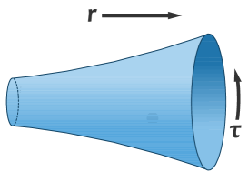
(a) thermal AdS

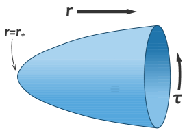
(b) AdS-Schwarzschild

Figure 7: The topology of the thermal AdS geometry and the AdS-Schwarzschild geometry.

For the low-temperature phase, the space is $X_{1}$ and the geometry is the thermal AdS with topology $S^{1}\times B^{4}$. Then the loop $C$ is never contracted to zero in $X_{1}$ and $C$ is not a boundary of any string worldsheet $D$, see Figure 7(a). This immediately implies that

$$\langle{\cal P}\rangle=0$$ (F.15)

in the large $N_{c}$ limit. Thus at the low-temperature, the thermal AdS geometry is stable and the configuration $X_{1}$ corresponds to the confined phase.

On the other hand, for the high-temperature phase, the relevant space is $X_{2}$ and the geometry is the AdS-Schwarzschild black hole with topology $R^{2}\times S^{3}$. In this case, the loop $C$ can be a boundary of a string worldsheet $D=B^{2}$, see Figure 7(b). Then the (regularized) area of the surface gives the non-zero Polyakov loop expectation value,

$$\langle{\cal P}\rangle\neq 0.$$ (F.16)

Therefore, at the high-temperature, the the AdS-Schwarzschild black hole geometry is more stable and the configuration $X_{2}$ corresponds to the deconfined phase.

References

- [1] J. M. Maldacena, “The Large N limit of superconformal field theories and supergravity,” Adv. Theor. Math. Phys. 2, 231-252 (1998). [arXiv:hep-th/9711200].
- [2] S. S. Gubser, I. R. Klebanov, A. M. Polyakov, “Gauge theory correlators from noncritical string theory,” Phys. Lett. B428, 105-114 (1998). [arXiv:hep-th/9802109].
- [3] E. Witten, “Anti-de Sitter space and holography,” Adv. Theor. Math. Phys. 2, 253-291 (1998). [arXiv:hep-th/9802150].
- [4] J. Polchinski, “Dirichlet Branes and Ramond-Ramond charges,” Phys. Rev. Lett. 75, 4724-4727 (1995). [arXiv:hep-th/9510017].
- [5] R. G. Leigh, “Dirac-Born-Infeld Action from Dirichlet Sigma Model,” Mod. Phys. Lett. A4, 2767 (1989).
- [6] E. Witten, “Bound states of strings and p-branes,” Nucl. Phys. B460, 335-350 (1996). [arXiv:hep-th/9510135].
- [7] G. W. Gibbons, K. -i. Maeda, “Black Holes and Membranes in Higher Dimensional Theories with Dilaton Fields,” Nucl. Phys. B298, 741 (1988).
- [8] D. Garfinkle, G. T. Horowitz, A. Strominger, “Charged black holes in string theory,” Phys. Rev. D43, 3140 (1991).
- [9] G. T. Horowitz, A. Strominger, “Black strings and P-branes,” Nucl. Phys. B360, 197-209 (1991).
- [10] L. Susskind, E. Witten, “The Holographic bound in anti-de Sitter space,” [arXiv:hep-th/9805114].
- [11] A. W. Peet, J. Polchinski, “UV / IR relations in AdS dynamics,” Phys. Rev. D59, 065011 (1999). [arXiv:hep-th/9809022].
- [12] E. Witten, “Anti-de Sitter space, thermal phase transition, and confinement in gauge theories,” Adv. Theor. Math. Phys. 2, 505 (1998) [arXiv:hep-th/9803131].
- [13] I. R. Klebanov and E. Witten, “AdS/CFT correspondence and symmetry breaking,” Nucl. Phys. B 556, 89 (1999) [arXiv:hep-th/9905104].
- [14] I. R. Klebanov and M. J. Strassler, “Supergravity and a confining gauge theory: Duality cascades and chi SB resolution of naked singularities,” JHEP 0008, 052 (2000) [arXiv:hep-th/0007191].
- [15] J. M. Maldacena and C. Nunez, “Towards the large N limit of pure N=1 superYang-Mills,” Phys. Rev. Lett. 86, 588 (2001) [arXiv:hep-th/0008001].
- [16] J. Polchinski and M. J. Strassler, “Hard scattering and gauge/string duality,” Phys. Rev. Lett. 88, 031601 (2002) [arXiv:hep-th/0109174].
- [17] A. Karch and E. Katz, “Adding flavor to AdS/CFT,” JHEP 0206, 043 (2002) [arXiv:hep-th/0205236].
- [18] J. Babington, J. Erdmenger, N. J. Evans, Z. Guralnik and I. Kirsch, “Chiral symmetry breaking and pions in nonsupersymmetric gauge/gravity duals,” Phys. Rev. D 69, 066007 (2004) [arXiv:hep-th/0306018].
- [19] M. Kruczenski, D. Mateos, R. C. Myers and D. J. Winters, “Towards a holographic dual of large N(c) QCD,” JHEP 0405, 041 (2004) [arXiv:hep-th/0311270].
- [20] D. Mateos, R. C. Myers and R. M. Thomson, “Thermodynamics of the brane,” JHEP 0705, 067 (2007) [arXiv:hep-th/0701132].
- [21] T. Sakai and S. Sugimoto, “Low energy hadron physics in holographic QCD,” Prog. Theor. Phys. 113, 843 (2005) [arXiv:hep-th/0412141].
- [22] T. Sakai, S. Sugimoto, “More on a holographic dual of QCD,” Prog. Theor. Phys. 114, 1083 (2005). [arXiv:hep-th/0507073].
- [23] J. Erlich, E. Katz, D. T. Son and M. A. Stephanov, “QCD and a holographic model of hadrons,” Phys. Rev. Lett. 95, 261602 (2005) [arXiv:hep-ph/0501128].
- [24] L. Da Rold and A. Pomarol, “Chiral symmetry breaking from five dimensional spaces,” Nucl. Phys. B 721, 79 (2005) [arXiv:hep-ph/0501218].
- [25] J. Hirn, N. Rius and V. Sanz, “Geometric approach to condensates in holographic QCD,” Phys. Rev. D 73, 085005 (2006) [arXiv:hep-ph/0512240].
- [26] S. J. Brodsky and G. F. de Teramond, “Hadronic spectra and light-front wavefunctions in holographic QCD,” Phys. Rev. Lett. 96, 201601 (2006) [arXiv:hep-ph/0602252].
- [27] S. J. Brodsky, G. F. de Teramond, “QCD and Light-Front Holography,” Acta Phys. Polon. B41, 2605-2643 (2010). [arXiv:1009.4232 [hep-ph]].
- [28] G. F. de Teramond, S. J. Brodsky, “Light-Front Quantization and AdS/QCD: An Overview,” J. Phys. Conf. Ser. 287, 012007 (2011). [arXiv:1103.1100 [hep-ph]].
- [29] S. J. Brodsky, F. -G. Cao, G. F. de Teramond, “AdS/QCD and Applications of Light-Front Holography,” [arXiv:1108.5718 [hep-ph]].
- [30] S. S. Afonin, “Holographic like models as a five-dimensional rewriting of large-Nc QCD,” Int. J. Mod. Phys. A 25 (2010) 5683 [arXiv:1001.3105 [hep-ph]].
- [31] V. Koch, “Aspects of chiral symmetry,” Int. J. Mod. Phys. E6, 203-250 (1997). [arXiv:nucl-th/9706075].
- [32] Y. Kim, “AdS/QCD at finite density and temperature,” Contributed to 6th International Workshop on Critical Point and Onset of Deconfinement, 23 - 29 Aug. 2010 at Joint Institute for Nuclear Research.
- [33] A. Karch, E. Katz, D. T. Son and M. A. Stephanov, “Linear confinement and AdS/QCD,” Phys. Rev. D 74, 015005 (2006) [arXiv:hep-ph/0602229].
- [34] J. B. Kogut, M. A. Stephanov and D. Toublan, “On two color QCD with baryon chemical potential,” Phys. Lett. B 464, 183 (1999) [arXiv:hep-ph/9906346]; D. T. Son and M. A. Stephanov, “QCD at finite isospin density,” Phys. Rev. Lett. 86, 592 (2001) [arXiv:hep-ph/0005225].
- [35] M. A. Shifman, A. I. Vainshtein and V. I. Zakharov, “QCD and Resonance Physics. Sum Rules,” Nucl. Phys. B 147, 385 (1979).
- [36] G. Boyd, J. Engels, F. Karsch, E. Laermann, C. Legeland, M. Lutgemeier and B. Petersson, “Thermodynamics of SU(3) lattice gauge theory,” Nucl. Phys. B 469, 419 (1996) [arXiv:hep-lat/9602007]; D. E. Miller, “Lattice QCD Calculation for the Physical Equation of State,” Phys. Rept. 443, 55 (2007) [arXiv:hep-ph/0608234].
- [37] K. Morita and S. H. Lee, “Mass shift and width broadening of J/psi in QGP from QCD sum rule,” Phys. Rev. Lett. 100, 022301 (2008) [arXiv:0704.2021 [nucl-th]].
- [38] S. S. Gubser, “Dilaton driven confinement,” [arXiv:hep-th/9902155]; A. Kehagias, K. Sfetsos, “On Running couplings in gauge theories from type IIB supergravity,” Phys. Lett. B454, 270-276 (1999). [arXiv:hep-th/9902125].
- [39] C. Csaki, M. Reece, “Toward a systematic holographic QCD: A Braneless approach,” JHEP 0705, 062 (2007). [arXiv:hep-ph/0608266].
- [40] O. Andreev, V. I. Zakharov, “Gluon Condensate, Wilson Loops and Gauge/String Duality,” Phys. Rev. D76, 047705 (2007). [arXiv:hep-ph/0703010].
- [41] H.-Ch. Kim and Y. Kim, “Quark-gluon mixed condensate of the QCD vacuum in Holographic QCD,” JHEP 0810, 011 (2008) [arXiv:0808.3639 [hep-ph]].
- [42] O. Andreev, “Nonlocal and Mixed Condensates Tests of Gauge/String Duality,” Phys. Rev. D 82, 086012 (2010) [arXiv:1008.4738 [hep-ph]].
- [43] V. M. Belyaev, B. L. Ioffe, “Determination of Baryon and Baryonic Resonance Masses from QCD Sum Rules. 1. Nonstrange Baryons,” Sov. Phys. JETP 56, 493-501 (1982).
- [44] H. Fritzsch and P. Minkowski, “Psi Resonances, Gluons and the Zweig Rule,” Nuovo Cim. A 30, 393 (1975).
- [45] R. L. Jaffe and K. Johnson, “Unconventional States of Confined Quarks and Gluons,” Phys. Lett. B 60, 201 (1976).
- [46] V. Mathieu, N. Kochelev, V. Vento, “The Physics of Glueballs,” Int. J. Mod. Phys. E18, 1-49 (2009). [arXiv:0810.4453 [hep-ph]].
- [47] V. Crede, C. A. Meyer, “The Experimental Status of Glueballs,” Prog. Part. Nucl. Phys. 63, 74-116 (2009). [arXiv:0812.0600 [hep-ex]].
- [48] C. Csaki, H. Ooguri, Y. Oz, J. Terning, “Glueball mass spectrum from supergravity,” JHEP 9901, 017 (1999). [arXiv:hep-th/9806021].
- [49] R. C. Brower, S. D. Mathur, C. -ITan, “Glueball spectrum for QCD from AdS supergravity duality,” Nucl. Phys. B587, 249-276 (2000). [arXiv:hep-th/0003115].
- [50] H. Boschi-Filho, N. R. F. Braga, “QCD / string holographic mapping and glueball mass spectrum,” Eur. Phys. J. C32, 529-533 (2004). [arXiv:hep-th/0209080]; H. Boschi-Filho, N. R. F. Braga, “Gauge / string duality and scalar glueball mass ratios,” JHEP 0305, 009 (2003). [arXiv:hep-th/0212207].
- [51] P. Colangelo, F. De Fazio, F. Jugeau, S. Nicotri, “On the light glueball spectrum in a holographic description of QCD,” Phys. Lett. B652, 73-78 (2007). [arXiv:hep-ph/0703316].
- [52] H. Forkel, “Holographic glueball structure,” Phys. Rev. D78, 025001 (2008). [arXiv:0711.1179 [hep-ph]].
- [53] P. Colangelo, F. Giannuzzi and S. Nicotri, “Holographic Approach to Finite Temperature QCD: The Case of Scalar Glueballs and Scalar Mesons,” Phys. Rev. D 80, 094019 (2009) [arXiv:0909.1534 [hep-ph]].
- [54] A. S. Miranda, C. A. Ballon Bayona, H. Boschi-Filho and N. R. F. Braga, “Black-hole quasinormal modes and scalar glueballs in a finite-temperature AdS/QCD model,” JHEP 0911, 119 (2009) [arXiv:0909.1790 [hep-th]].
- [55] D. T. Son and A. O. Starinets, “Minkowski-space correlators in AdS/CFT correspondence: recipe and applications,” JHEP 0209, 042 (2002) [arXiv:hep-th/0205051].
- [56] C. P. Herzog, “A Holographic Prediction of the Deconfinement Temperature,” Phys. Rev. Lett. 98, 091601 (2007). [arXiv:hep-th/0608151].
- [57] J. P. Shock, F. Wu, Y. L. Wu and Z. F. Xie, “AdS/QCD Phenomenological Models from a Back-Reacted Geometry,” JHEP 0703, 064 (2007) [arXiv:hep-ph/0611227].
- [58] W. de Paula, T. Frederico, H. Forkel and M. Beyer, “Dynamical AdS/QCD with area-law confinement and linear Regge trajectories,” Phys. Rev. D 79 (2009) 075019 [arXiv:0806.3830 [hep-ph]].
- [59] C. Amsler et al. [ Particle Data Group Collaboration ], “Review of Particle Physics,” Phys. Lett. B667, 1-1340 (2008).
- [60] J. Erlich and C. Westenberger, “Tests of Universality in AdS/QCD,” Phys. Rev. D 79, 066014 (2009) [arXiv:0812.5105 [hep-ph]].
- [61] D. K. Hong, T. Inami and H. U. Yee, “Baryons in AdS/QCD,” Phys. Lett. B 646, 165 (2007) [arXiv:hep-ph/0609270].
- [62] N. Maru and M. Tachibana, “Meson-Nucleon Coupling from AdS/QCD,” Eur. Phys. J. C 63, 123 (2009) [arXiv:0904.3816 [hep-ph]].
- [63] H. C. Kim, Y. Kim and U. Yakhshiev, “Mesons and nucleons from holographic QCD in a unified approach,” JHEP 0911, 034 (2009) [arXiv:0908.3406 [hep-ph]].
- [64] P. Zhang, “Improving the Excited Nucleon Spectrum in Hard-Wall AdS/QCD,” Phys. Rev. D 81, 114029 (2010) [arXiv:1002.4352 [hep-ph]].
- [65] B. Batell and T. Gherghetta, “Dynamical Soft-Wall AdS/QCD,” Phys. Rev. D 78, 026002 (2008) [arXiv:0801.4383 [hep-ph]].
- [66] T. Gherghetta, J. I. Kapusta and T. M. Kelley, “Chiral symmetry breaking in the soft-wall AdS/QCD model,” Phys. Rev. D 79, 076003 (2009) [arXiv:0902.1998 [hep-ph]].
- [67] P. Colangelo, F. De Fazio, F. Giannuzzi, F. Jugeau and S. Nicotri, “Light scalar mesons in the soft-wall model of AdS/QCD,” Phys. Rev. D 78, 055009 (2008) [arXiv:0807.1054 [hep-ph]].
- [68] Y. Q. Sui, Y. L. Wu, Z. F. Xie and Y. B. Yang, “Prediction for the Mass Spectra of Resonance Mesons in the Soft-Wall AdS/QCD with a Modified 5D Metric,” Phys. Rev. D 81, 014024 (2010) [arXiv:0909.3887 [hep-ph]].
- [69] M. Shifman and A. Vainshtein, “Highly Excited Mesons, Linear Regge Trajectories and the Pattern of the Chiral Symmetry Realization,” Phys. Rev. D 77, 034002 (2008) [arXiv:0710.0863 [hep-ph]].
- [70] N. Evans and A. Tedder, “Perfecting the Ultra-violet of Holographic Descriptions of QCD,” Phys. Lett. B 642, 546 (2006) [arXiv:hep-ph/0609112].
- [71] S. S. Afonin, “Low-energy holographic models for QCD,” Phys. Rev. C 83 (2011) 048202 [arXiv:1102.0156 [hep-ph]].
- [72] H. Forkel, “Light scalar tetraquarks from a holographic perspective,” Phys. Lett. B 694 (2010) 252 [arXiv:1007.4341 [hep-ph]].
- [73] A. Bertin et al. [OBELIX Collaboration], “Study of anti-p p –¿ 2pi+ 2pi- annihilation from S states,” Phys. Lett. B 414, 220 (1997).
- [74] M. Harada, S. Matsuzaki and K. Yamawaki, “Implications of Holographic QCD in ChPT with Hidden Local Symmetry,” Phys. Rev. D 74, 076004 (2006) [arXiv:hep-ph/0603248].
- [75] K. Nawa, H. Suganuma and T. Kojo, “Baryons in holographic QCD,” Phys. Rev. D 75, 086003 (2007) [arXiv:hep-th/0612187].
- [76] D. K. Hong, M. Rho, H. U. Yee and P. Yi, “Chiral Dynamics of Baryons from String Theory,” Phys. Rev. D 76, 061901 (2007) [arXiv:hep-th/0701276].
- [77] H. Hata, T. Sakai, S. Sugimoto and S. Yamato, “Baryons from instantons in holographic QCD,” Prog. Theor. Phys. 117, 1157 (2007) [arXiv:hep-th/0701280].
- [78] D. K. Hong, M. Rho, H. U. Yee and P. Yi, “Nucleon form-factors and hidden symmetry in holographic QCD,” Phys. Rev. D 77, 014030 (2008) [arXiv:0710.4615 [hep-ph]].
- [79] K. Hashimoto, T. Sakai and S. Sugimoto, “Holographic Baryons: Static Properties and Form Factors from Gauge/String Duality,” Prog. Theor. Phys. 120, 1093 (2008) [arXiv:0806.3122 [hep-th]].
- [80] M. Harada, S. Matsuzaki and K. Yamawaki, “Holographic QCD Integrated back to Hidden Local Symmetry,” Phys. Rev. D 82, 076010 (2010) [arXiv:1007.4715 [hep-ph]].
- [81] M. Harada and M. Rho, “Integrating Holographic Vector Dominance to Hidden Local Symmetry for the Nucleon Form Factor,” [arXiv:1102.5489 [hep-ph]].
- [82] A. Pomarol and A. Wulzer, “Baryon Physics in Holographic QCD,” Nucl. Phys. B 809, 347 (2009) [arXiv:0807.0316 [hep-ph]].
- [83] N. Brambilla et al., “Heavy quarkonium: progress, puzzles, and opportunities,” Eur. Phys. J. C 71, 1534 (2011) [arXiv:1010.5827 [hep-ph]].
- [84] Y. Kim, J. P. Lee and S. H. Lee, “Heavy quarkonium in a holographic QCD model,” Phys. Rev. D 75, 114008 (2007) [arXiv:hep-ph/0703172].
- [85] M. Fujita, K. Fukushima, T. Misumi and M. Murata, “Finite-temperature spectral function of the vector mesons in an AdS/QCD model,” Phys. Rev. D 80, 035001 (2009) [arXiv:0903.2316 [hep-ph]].
- [86] R. C. Myers, A. O. Starinets and R. M. Thomson, “Holographic spectral functions and diffusion constants for fundamental matter,” JHEP 0711, 091 (2007) [arXiv:0706.0162 [hep-th]].
- [87] H. Liu, K. Rajagopal and U. A. Wiedemann, “An AdS/CFT Calculation of Screening in a Hot Wind,” Phys. Rev. Lett. 98, 182301 (2007) [arXiv:hep-ph/0607062].
- [88] R. C. Myers and A. Sinha, “The Fast life of holographic mesons,” JHEP 0806, 052 (2008) [arXiv:0804.2168 [hep-th]].
- [89] H. R. Grigoryan, P. M. Hohler and M. A. Stephanov, “Towards the Gravity Dual of Quarkonium in the Strongly Coupled QCD Plasma,” Phys. Rev. D 82, 026005 (2010) [arXiv:1003.1138 [hep-ph]].
- [90] An incomplete list: J. M. Maldacena, “Wilson loops in large N field theories,” Phys. Rev. Lett. 80, 4859 (1998) [arXiv:hep-th/9803002]; S. J. Rey, S. Theisen and J. T. Yee, “Wilson-Polyakov loop at finite temperature in large N gauge theory and anti-de Sitter supergravity,” Nucl. Phys. B 527, 171 (1998) [arXiv:hep-th/9803135]; O. Andreev and V. I. Zakharov, “Heavy-quark potentials and AdS/QCD,” Phys. Rev. D 74, 025023 (2006) [arXiv:hep-ph/0604204]; H. Boschi-Filho, N. R. F. Braga and C. N. Ferreira, “Heavy quark potential at finite temperature from gauge/string duality,” Phys. Rev. D 74, 086001 (2006) [arXiv:hep-th/0607038]; O. Andreev and V. I. Zakharov, “On Heavy-Quark Free Energies, Entropies, Polyakov Loop, and AdS/QCD,” JHEP 0704 (2007) 100 [arXiv:hep-ph/0611304]; C. D. White, “The Cornell potential from general geometries in AdS/QCD,” Phys. Lett. B 652, 79 (2007) [arXiv:hep-ph/0701157]; D. Hou and H. c. Ren, “Heavy Quarkonium States with the Holographic Potential,” JHEP 0801, 029 (2008) [arXiv:0710.2639 [hep-ph]]; Y. Kim, B. H. Lee, C. Park and S. J. Sin, “The Effect of gluon condensate on holographic heavy quark potential,” Phys. Rev. D 80, 105016 (2009) [arXiv:0808.1143 [hep-th]]; M. Mia, K. Dasgupta, C. Gale and S. Jeon, “Toward Large N Thermal QCD from Dual Gravity: The Heavy Quarkonium Potential,” Phys. Rev. D 82, 026004 (2010) [arXiv:1004.0387 [hep-th]]; S. He, M. Huang and Q. S. Yan, “Logarithmic correction in the deformed AdS5 model to produce the heavy quark potential and QCD beta function,” Phys. Rev. D 83, 045034 (2011) [arXiv:1004.1880 [hep-ph]]; H. R. Grigoryan and Y. V. Kovchegov, “Gravity Dual Corrections to the Heavy Quark Potential at Finite-Temperature,” [arXiv:1105.2300 [hep-th]].
- [91] D. Hou and H. c. Ren, “Heavy Quarkonium States with the Holographic Potential,” JHEP 0801, 029 (2008) [arXiv:0710.2639 [hep-ph]];
- [92] S. Eidelman et al. [ Particle Data Group Collaboration ], “Review of particle physics. Particle Data Group,” Phys. Lett. B592, 1 (2004).
- [93] L. J. Reinders, H. Rubinstein and S. Yazaki, “Hadron Properties from QCD Sum Rules,” Phys. Rept. 127, 1 (1985); T. Ericson and W. Weise, “Pions and nuclei,” Oxford University Press, Oxford U.K. (1988); G. F. Sterman and P. Stoler, “Hadronic form-factors and perturbative QCD,” Ann. Rev. Nucl. Part. Sci. 47, 193 (1997) [arXiv:hep-ph/9708370].
- [94] H. R. Grigoryan and A. V. Radyushkin, “Form Factors and Wave Functions of Vector Mesons in Holographic QCD,” Phys. Lett. B 650, 421 (2007) [arXiv:hep-ph/0703069].
- [95] H. R. Grigoryan and A. V. Radyushkin, “Structure of vector mesons in holographic model with linear confinement,” Phys. Rev. D 76, 095007 (2007) [arXiv:0706.1543 [hep-ph]].
- [96] F. T. Hawes and M. A. Pichowsky, “Electromagnetic form-factors of light vector mesons,” Phys. Rev. C 59, 1743 (1999) [arXiv:nucl-th/9806025].
- [97] M. S. Bhagwat and P. Maris, “Vector meson form factors and their quark-mass dependence,” Phys. Rev. C 77, 025203 (2008) [arXiv:nucl-th/0612069].
- [98] J. N. Hedditch, W. Kamleh, B. G. Lasscock, D. B. Leinweber, A. G. Williams and J. M. Zanotti, “Pseudoscalar and vector meson form-factors from lattice QCD,” Phys. Rev. D 75, 094504 (2007) [arXiv:hep-lat/0703014].
- [99] H. R. Grigoryan and A. V. Radyushkin, “Pion form-factor in chiral limit of hard-wall AdS/QCD model,” Phys. Rev. D 76, 115007 (2007) [arXiv:0709.0500 [hep-ph]].
- [100] H. J. Kwee and R. F. Lebed, “Pion Form Factor in Improved Holographic QCD Backgrounds,” Phys. Rev. D 77, 115007 (2008) [arXiv:0712.1811 [hep-ph]].
- [101] Z. Abidin and C. E. Carlson, “Gravitational form factors of vector mesons in an AdS/QCD model,” Phys. Rev. D 77, 095007 (2008) [arXiv:0801.3839 [hep-ph]].
- [102] Z. Abidin and C. E. Carlson, “Gravitational Form Factors in the Axial Sector from an AdS/QCD Model,” Phys. Rev. D 77, 115021 (2008) [arXiv:0804.0214 [hep-ph]].
- [103] H. R. Grigoryan and A. V. Radyushkin, “Anomalous Form Factor of the Neutral Pion in Extended AdS/QCD Model with Chern-Simons Term,” Phys. Rev. D 77, 115024 (2008) [arXiv:0803.1143 [hep-ph]].
- [104] Z. Abidin and C. E. Carlson, “Nucleon electromagnetic and gravitational form factors from holography,” Phys. Rev. D 79, 115003 (2009) [arXiv:0903.4818 [hep-ph]].
- [105] S. J. Brodsky, F. G. Cao and G. F. de Teramond, “Meson Transition Form Factors in Light-Front Holographic QCD,” [arXiv:1105.3999 [hep-ph]].
- [106] F. Zuo and T. Huang, “Photon-to-pion transition form factor and pion distribution amplitude from holographic QCD,” [arXiv:1105.6008 [hep-ph]].
- [107] C. A. Ballon Bayona, H. Boschi-Filho, N. R. F. Braga and M. A. C. Torres, “Form factors of vector and axial-vector mesons in holographic D4-D8 model,” JHEP 1001, 052 (2010) [arXiv:0911.0023 [hep-th]].
- [108] F. Karsch, “Lattice QCD at high temperature and the QGP,” AIP Conf. Proc. 842, 20 (2006) [arXiv:hep-lat/0601013]; M. A. Stephanov, “QCD phase diagram: An Overview,” PoS LAT2006, 024 (2006) [arXiv:hep-lat/0701002]; Z. Fodor and S. D. Katz, “The Phase diagram of quantum chromodynamics,” [arXiv:0908.3341 [hep-ph]]; R. Stock, “The QCD Phase Diagram: Expectations and Challenges,” PoS C POD2009, 001 (2009) [arXiv:0909.0601 [nucl-ex]]; K. Fukushima and T. Hatsuda, “The phase diagram of dense QCD,” Rept. Prog. Phys. 74, 014001 (2011) [arXiv:1005.4814 [hep-ph]].
- [109] L. D. McLerran, “A Chiral Symmetry Order Parameter, the Lattice and Nucleosynthesis,” Phys. Rev. D36, 3291 (1987).
- [110] S. Jeon, V. Koch, “Charged particle ratio fluctuation as a signal for QGP,” Phys. Rev. Lett. 85, 2076-2079 (2000). [arXiv:hep-ph/0003168]; M. Asakawa, U. W. Heinz, B. Muller, “Fluctuation probes of quark deconfinement,” Phys. Rev. Lett. 85, 2072-2075 (2000). [arXiv:hep-ph/0003169]; M. Prakash, I. Zahed, “Quark susceptibility in hot QCD,” Phys. Rev. Lett. 69, 3282-3285 (1992).
- [111] S. A. Gottlieb, W. Liu, D. Toussaint, R. L. Renken, R. L. Sugar, “The Quark Number Susceptibility of High Temperature QCD,” Phys. Rev. Lett. 59, 2247 (1987).
- [112] S. W. Hawking, D. N. Page, “Thermodynamics of Black Holes in anti-De Sitter Space,” Commun. Math. Phys. 87, 577 (1983).
- [113] C. A. Ballon Bayona, H. Boschi-Filho, N. R. F. Braga and L. A. Pando Zayas, “On a Holographic Model for Confinement/Deconfinement,” Phys. Rev. D 77, 046002 (2008) [arXiv:0705.1529 [hep-th]].
- [114] R. G. Cai and J. P. Shock, “Holographic confinement/deconfinement phase transitions of AdS/QCD in curved spaces,” JHEP 0708, 095 (2007) [arXiv:0705.3388 [hep-th]].
- [115] A. Chamblin, R. Emparan, C. V. Johnson and R. C. Myers, “Charged AdS black holes and catastrophic holography,” Phys. Rev. D 60, 064018 (1999) [arXiv:hep-th/9902170].
- [116] N. Evans and E. Threlfall, “The Thermal phase transition in a QCD-like holographic model,” Phys. Rev. D 78, 105020 (2008) [arXiv:0805.0956 [hep-th]].
- [117] Y. Kim, B. H. Lee, S. Nam, C. Park and S. J. Sin, “Deconfinement phase transition in holographic QCD with matter,” Phys. Rev. D 76, 086003 (2007) [arXiv:0706.2525 [hep-ph]].
- [118] S. J. Sin, “Gravity back-reaction to the baryon density for bulk filling branes,” JHEP 0710, 078 (2007) [arXiv:0707.2719 [hep-th]]; B. H. Lee, C. Park and S. J. Sin, “A Dual Geometry of the Hadron in Dense Matter,” JHEP 0907, 087 (2009) [arXiv:0905.2800 [hep-th]]; C. Park, D. Y. Gwak, B. H. Lee, Y. Ko and S. Shin, “The Soft Wall Model in the Hadronic Medium,” [arXiv:1104.4182 [hep-th]].
- [119] R. G. Cai and N. Ohta, “Deconfinement Transition of AdS/QCD at O(alpha-prime**3),” Phys. Rev. D 76, 106001 (2007) [arXiv:0707.2013 [hep-th]].
- [120] U. Gursoy, E. Kiritsis, L. Mazzanti and F. Nitti, “Holography and Thermodynamics of 5D Dilaton-gravity,” JHEP 0905, 033 (2009) [arXiv:0812.0792 [hep-th]].
- [121] O. Andreev, “Renormalized Polyakov Loop in the Deconfined Phase of SU(N) Gauge Theory and Gauge/String Duality,” Phys. Rev. Lett. 102 (2009) 212001 [arXiv:0903.4375 [hep-ph]].
- [122] A. Gocksch and F. Neri, “On Large N QCD At Finite Temperature,” Phys. Rev. Lett. 50, 1099 (1983).
- [123] F. Neri and A. Gocksch, “Chiral symmetry restoration in large N QCD at finite temperature,” Phys. Rev. D 28, 3147 (1983).
- [124] R. D. Pisarski, “Finite Temperature QCD At Large N,” Phys. Rev. D 29, 1222 (1984).
- [125] Y. Kim and H. K. Lee, “Consequences of the partial restoration of chiral symmetry in AdS/QCD,” Phys. Rev. D 77, 096011 (2008) [arXiv:0802.2409 [hep-ph]].
- [126] K. Jo, Y. Kim, H. K. Lee and S. J. Sin, “Quark number Susceptibility and Phase Transition in hQCD Models,” JHEP 0811, 040 (2008) [arXiv:0810.0063 [hep-ph]], note that the arXiv version of this paper is the latest one.
- [127] K. Ghoroku and M. Yahiro, “Holographic model for mesons at finite temperature,” Phys. Rev. D 73, 125010 (2006) [arXiv:hep-ph/0512289].
- [128] O. Aharony, J. Sonnenschein and S. Yankielowicz, “A Holographic model of deconfinement and chiral symmetry restoration,” Annals Phys. 322, 1420 (2007) [arXiv:hep-th/0604161].
- [129] N. Evans, A. Gebauer, K. Y. Kim and M. Magou, “Holographic Description of the Phase Diagram of a Chiral Symmetry Breaking Gauge Theory,” JHEP 1003, 132 (2010) [arXiv:1002.1885 [hep-th]].
- [130] N. Evans, A. Gebauer and K. Y. Kim, “E, B, , T Phase Structure of the D3/D7 Holographic Dual,” JHEP 1105, 067 (2011) [arXiv:1103.5627 [hep-th]].
- [131] S. de Haro, S. N. Solodukhin and K. Skenderis, “Holographic reconstruction of space-time and renormalization in the AdS/CFT correspondence,” Commun. Math. Phys. 217, 595 (2001) [arXiv:hep-th/0002230].
- [132] R. A. Janik and R. B. Peschanski, “Asymptotic perfect fluid dynamics as a consequence of Ads/CFT,” Phys. Rev. D 73, 045013 (2006) [arXiv:hep-th/0512162].
- [133] C. Fefferman and C. R. Graham, “Conformal Invariants,” Élie Cartan et les mathématiques d’aujourd’hui, Astérisque, No.Hors Sér. 1985, 95-116 (1985).
- [134] K. Kajantie, T. Tahkokallio and J. T. Yee, “Thermodynamics of AdS/QCD,” JHEP 0701, 019 (2007) [arXiv:hep-ph/0609254]; O. Andreev, “Some Thermodynamic Aspects of Pure Glue, Fuzzy Bags and Gauge/String Duality,” Phys. Rev. D 76 (2007) 087702 [arXiv:0706.3120 [hep-ph]]; S. S. Gubser and A. Nellore, “Mimicking the QCD equation of state with a dual black hole,” Phys. Rev. D 78, 086007 (2008) [arXiv:0804.0434 [hep-th]]; U. Gursoy, E. Kiritsis, L. Mazzanti and F. Nitti, “Holography and Thermodynamics of 5D Dilaton-gravity,” JHEP 0905, 033 (2009) [arXiv:0812.0792 [hep-th]]; D. Li, S. He, M. Huang, Q. -S. Yan, “Thermodynamics of deformed AdS5 model with a positive/negative quadratic correction in graviton-dilaton system,” [arXiv:1103.5389 [hep-th]].
- [135] U. Gursoy, E. Kiritsis, L. Mazzanti and F. Nitti, “Deconfinement and Gluon Plasma Dynamics in Improved Holographic QCD,” Phys. Rev. Lett. 101, 181601 (2008) [arXiv:0804.0899 [hep-th]].
- [136] U. Gursoy and E. Kiritsis, “Exploring improved holographic theories for QCD: Part I,” JHEP 0802, 032 (2008) [arXiv:0707.1324 [hep-th]]; U. Gursoy, E. Kiritsis and F. Nitti, “Exploring improved holographic theories for QCD: Part II,” JHEP 0802, 019 (2008) [arXiv:0707.1349 [hep-th]].
- [137] M. Panero, “Thermodynamics of the QCD plasma and the large-N limit,” Phys. Rev. Lett. 103 (2009) 232001. [arXiv:0907.3719 [hep-lat]].
- [138] Y. Kim, Y. Matsuo, W. Sim, S. Takeuchi and T. Tsukioka, “Quark Number Susceptibility with Finite Chemical Potential in Holographic QCD,” JHEP 1005, 038 (2010) [arXiv:1001.5343 [hep-th]].
- [139] K. -i. Kim, Y. Kim, S. Takeuchi, T. Tsukioka, “Quark Number Susceptibility with Finite Quark Mass in Holographic QCD,” [arXiv:1012.2667 [hep-ph]], to appear in Prog. Theor. Phys. (2011).
- [140] T. Kunihiro, “Quark number susceptibility and fluctuations in the vector channel at high temperatures,” Phys. Lett. B 271, 395 (1991).
- [141] A. Stoffers and I. Zahed, “Improved AdS/QCD Model with Matter,” Phys. Rev. D 83, 055016 (2011) [arXiv:1009.4428 [hep-th]].
- [142] O. DeWolfe, S. S. Gubser and C. Rosen, “A holographic critical point,” Phys. Rev. D 83, 086005 (2011) [arXiv:1012.1864 [hep-th]].
- [143] J. D. Walecka, “A Theory of highly condensed matter,” Annals Phys. 83, 491 (1974); B. D. Serot and J. D. Walecka, “The Relativistic Nuclear Many Body Problem,” Adv. Nucl. Phys. 16, 1 (1986).
- [144] R. J. Furnstahl and B. D. Serot, “Quantum hadrodynamics: Evolution and revolution,” Comments Nucl. Part. Phys. 2, A23 (2000) [arXiv:nucl-th/0005072].
- [145] H. R. Grigoryan, “Dimension Six Correction to the Vector Sector of AdS/QCD Model,” Phys. Lett. B 662, 158 (2008) [arXiv:0709.0939 [hep-ph]]; Y. Kim, P. Ko and X. H. Wu, “Holographic QCD beyond the leading order,” JHEP 0806, 094 (2008) [arXiv:0804.2710 [hep-ph]].
- [146] K. K. Kim, Y. Kim and Y. Ko, “Self-bound dense objects in holographic QCD,” JHEP 1010, 039 (2010) [arXiv:1007.2470 [hep-ph]].
- [147] S. K. Domokos and J. A. Harvey, “Baryon number-induced Chern-Simons couplings of vector and axial-vector mesons in holographic QCD,” Phys. Rev. Lett. 99, 141602 (2007) [arXiv:0704.1604 [hep-ph]].
- [148] Y. Kim, C. H. Lee and H. U. Yee, “Holographic Nuclear Matter in AdS/QCD,” Phys. Rev. D 77, 085030 (2008) [arXiv:0707.2637 [hep-ph]].
- [149] B. H. Lee, C. Park and S. J. Sin, “A Dual Geometry of the Hadron in Dense Matter,” JHEP 0907, 087 (2009) [arXiv:0905.2800 [hep-th]];
- [150] K. Y. Kim, S. J. Sin and I. Zahed, “Dense hadronic matter in holographic QCD,” [arXiv:hep-th/0608046]; N. Horigome and Y. Tanii, “Holographic chiral phase transition with chemical potential,” JHEP 0701, 072 (2007) [arXiv:hep-th/0608198]; K. Y. Kim, S. J. Sin and I. Zahed, “The Chiral Model of Sakai-Sugimoto at Finite Baryon Density,” JHEP 0801, 002 (2008) [arXiv:0708.1469 [hep-th]]; M. Rozali, H. H. Shieh, M. Van Raamsdonk and J. Wu, “Cold Nuclear Matter In Holographic QCD,” JHEP 0801, 053 (2008) [arXiv:0708.1322 [hep-th]]; O. Bergman, G. Lifschytz and M. Lippert, “Holographic Nuclear Physics,” JHEP 0711, 056 (2007) [arXiv:0708.0326 [hep-th]].
- [151] M. Rozali, H. -H. Shieh, M. Van Raamsdonk, J. Wu, “Cold Nuclear Matter In Holographic QCD,” JHEP 0801, 053 (2008). [arXiv:0708.1322 [hep-th]].
- [152] S. Nakamura, Y. Seo, S. J. Sin and K. P. Yogendran, “A New Phase at Finite Quark Density from AdS/CFT,” J. Korean Phys. Soc. 52, 1734 (2008) [arXiv:hep-th/0611021]; S. Kobayashi, D. Mateos, S. Matsuura, R. C. Myers and R. M. Thomson, “Holographic phase transitions at finite baryon density,” JHEP 0702, 016 (2007) [arXiv:hep-th/0611099].
- [153] K. Y. Kim and I. Zahed, “Nucleon-Nucleon Potential from Holography,” JHEP 0903, 131 (2009) [arXiv:0901.0012 [hep-th]].
- [154] K. Hashimoto, T. Sakai and S. Sugimoto, “Nuclear Force from String Theory,” Prog. Theor. Phys. 122, 427 (2009) [arXiv:0901.4449 [hep-th]].
- [155] Y. Kim, S. Lee and P. Yi, “Holographic Deuteron and Nucleon-Nucleon Potential,” JHEP 0904, 086 (2009) [arXiv:0902.4048 [hep-th]].
- [156] Y. Kim, S. Lee and P. Yi, “Nucleon-nucleon potential in holographic QCD,” Nucl. Phys. A 844, 224C (2010).
- [157] J. Erdmenger, N. Evans, I. Kirsch and E. Threlfall, “Mesons in Gauge/Gravity Duals - A Review,” Eur. Phys. J. A 35, 81 (2008) [arXiv:0711.4467 [hep-th]]; R. Peschanski, “Introduction to String Theory and Gauge/Gravity duality for students in QCD and QGP phenomenology,” Acta Phys. Polon. B 39, 2479 (2008) [arXiv:0804.3210 [hep-ph]]; F. Jugeau, “Hadrons potentials within the gauge/string correspondence,” Annals Phys. 325, 1739 (2010) [arXiv:0812.4903 [hep-ph]]; S. S. Gubser and A. Karch, “From gauge-string duality to strong interactions: A Pedestrian’s Guide,” Ann. Rev. Nucl. Part. Sci. 59, 145 (2009) [arXiv:0901.0935 [hep-th]]; J. Erlich, “How Well Does AdS/QCD Describe QCD?,” Int. J. Mod. Phys. A 25, 411 (2010) [arXiv:0908.0312 [hep-ph]]; J. McGreevy, “Holographic duality with a view toward many-body physics,” Adv. High Energy Phys. 2010, 723105 (2010) [arXiv:0909.0518 [hep-th]]; C. Nunez, A. Paredes and A. V. Ramallo, “Unquenched flavor in the gauge/gravity correspondence,” Adv. High Energy Phys. 2010, 196714 (2010) [arXiv:1002.1088 [hep-th]]; U. Gursoy, E. Kiritsis, L. Mazzanti, G. Michalogiorgakis and F. Nitti, “Improved Holographic QCD,” Lect. Notes Phys. 828, 79 (2011) [arXiv:1006.5461 [hep-th]]; J. Casalderrey-Solana, H. Liu, D. Mateos, K. Rajagopal and U. A. Wiedemann, “Gauge/String Duality, Hot QCD and Heavy Ion Collisions,” [arXiv:1101.0618 [hep-th]]; G. F. de Teramond and S. J. Brodsky, “Light-Front Quantization and AdS/QCD: An Overview,” J. Phys. Conf. Ser. 287, 012007 (2011) [arXiv:1103.1100 [hep-ph]]; P. Yi, “Precision Holographic Baryons,” [arXiv:1103.1684 [nucl-th]].
- [158] J. Polchinski, M. J. Strassler, “Deep inelastic scattering and gauge/string duality,” JHEP 0305, 012 (2003). [arXiv:hep-th/0209211].
- [159] O. Andreev, “Scaling laws in hadronic processes and string theory,” Phys. Rev. D 67 (2003) 046001 [arXiv:hep-th/0209256].
- [160] Y. Hatta, E. Iancu and A. H. Mueller, “Deep inelastic scattering at strong coupling from gauge/string duality: The Saturation line,” JHEP 0801, 026 (2008) [arXiv:0710.2148 [hep-th]].
- [161] L. Cornalba and M. S. Costa, “Saturation in Deep Inelastic Scattering from AdS/CFT,” Phys. Rev. D 78, 096010 (2008) [arXiv:0804.1562 [hep-ph]].
- [162] J. L. Albacete, Y. V. Kovchegov and A. Taliotis, “DIS on a Large Nucleus in AdS/CFT,” JHEP 0807, 074 (2008) [arXiv:0806.1484 [hep-th]].
- [163] J. H. Gao and B. W. Xiao, “Polarized Deep Inelastic and Elastic Scattering From Gauge/String Duality,” Phys. Rev. D 80, 015025 (2009) [arXiv:0904.2870 [hep-ph]].
- [164] E. Avsar, E. Iancu, L. McLerran and D. N. Triantafyllopoulos, “Shockwaves and deep inelastic scattering within the gauge/gravity duality,” JHEP 0911, 105 (2009) [arXiv:0907.4604 [hep-th]].
- [165] C. A. Ballon Bayona, H. Boschi-Filho and N. R. F. Braga, “Deep Inelastic Scattering in Holographic AdS/QCD Models,” Nucl. Phys. Proc. Suppl. 199, 97 (2010) [arXiv:0910.1309 [hep-th]].
- [166] L. Cornalba, M. S. Costa and J. Penedones, “Deep Inelastic Scattering in Conformal QCD,” JHEP 1003 (2010) 133 [arXiv:0911.0043 [hep-th]].
- [167] J. H. Gao and Z. G. Mou, “Polarized Deep Inelastic Scattering Off the Neutron From Gauge/String Duality,” Phys. Rev. D 81, 096006 (2010) [arXiv:1003.3066 [hep-ph]].
- [168] L. Cornalba, M. S. Costa and J. Penedones, “AdS black disk model for small-x DIS,” Phys. Rev. Lett. 105 (2010) 072003 [arXiv:1001.1157 [hep-ph]].
- [169] R. C. Brower, M. Djuric, I. Sarcevic and C. I. Tan, “The AdS Graviton/Pomeron Description of Deep Inelastic Scattering at Small x,” [arXiv:1106.5681 [hep-ph]].
- [170] T. Branz, T. Gutsche, V. E. Lyubovitskij, I. Schmidt and A. Vega, “Light and heavy mesons in a soft-wall holographic approach,” Phys. Rev. D 82, 074022 (2010) [arXiv:1008.0268 [hep-ph]].
- [171] O. Andreev, “Some Multi-Quark Potentials, Pseudo-Potentials and AdS/QCD,” Phys. Rev. D 78 (2008) 065007 [arXiv:0804.4756 [hep-ph]].
- [172] M. V. Carlucci, F. Giannuzzi, G. Nardulli, M. Pellicoro and S. Stramaglia, “AdS-QCD quark-antiquark potential, meson spectrum and tetraquarks,” Eur. Phys. J. C 57, 569 (2008) [arXiv:0711.2014 [hep-ph]].
- [173] H. C. Kim and Y. Kim, “Hybrid exotic meson with J**PC = 1-+ in AdS/QCD,” JHEP 0901, 034 (2009) [arXiv:0811.0645 [hep-ph]].
- [174] F. Giannuzzi, “Doubly heavy baryons in a Salpeter model with AdS/QCD inspired potential,” Phys. Rev. D 79, 094002 (2009) [arXiv:0902.4624 [hep-ph]].
- [175] P. N. Kopnin, “Low-energy theorems and spectral density of the Dirac operator in AdS/QCD,” Phys. Rev. D 80, 126005 (2009) [arXiv:0907.1294 [hep-ph]].
- [176] N. Evans and A. Tedder, “A Holographic model of hadronization,” Phys. Rev. Lett. 100, 162003 (2008) [arXiv:0711.0300 [hep-ph]].
- [177] O. Andreev, “Cold Quark Matter, Quadratic Corrections and Gauge/String Duality,” Phys. Rev. D 81, 087901 (2010) [arXiv:1001.4414 [hep-ph]].
- [178] W. S. l’Yi, “Correlators of currents corresponding to the massive p-form fields in AdS/CFT correspondence,” Phys. Lett. B448, 218-226 (1999). [arXiv:hep-th/9811097].
- [179] M. Henningson, K. Sfetsos, “Spinors and the AdS/CFT correspondence,” Phys. Lett. B431, 63-68 (1998). [arXiv:hep-th/9803251].
- [180] G. E. Arutyunov, S. A. Frolov, “Antisymmetric tensor field on AdS(5),” Phys. Lett. B441, 173-177 (1998). [arXiv:hep-th/9807046].
- [181] A. Volovich, “Rarita-Schwinger field in the AdS/CFT correspondence,” JHEP 9809, 022 (1998). [arXiv:hep-th/9809009].
- [182] A. S. Koshelev, O. A. Rytchkov, “Note on the massive Rarita-Schwinger field in the AdS/CFT correspondence,” Phys. Lett. B450, 368-376 (1999). [arXiv:hep-th/9812238].
- [183] A. Polishchuk, “Massive symmetric tensor field on AdS,” JHEP 9907, 007 (1999). [arXiv:hep-th/9905048].
- [184] J. Polchinski, “String theory. Vol. 1: An introduction to the bosonic string,” Cambridge, UK: Univ. Pr. (1998).
- [185] K. Ghoroku, M. Ishihara, A. Nakamura, “Flavor quarks in AdS4 and gauge/gravity correspondence,” Phys. Rev. D75, 046005 (2007). [arXiv:hep-th/0612244].
- [186] M. Kruczenski, D. Mateos, R. C. Myers, D. J. Winters, “Meson spectroscopy in AdS/CFT with flavor,” JHEP 0307, 049 (2003). [arXiv:hep-th/0304032].
- [187] R. M. Wald, “General Relativity,” Chicago, Usa: Univ. Pr. (1984).
- [188] S. S. Gubser, A. Nellore, “Mimicking the QCD equation of state with a dual black hole,” Phys. Rev. D78, 086007 (2008). [arXiv:0804.0434 [hep-th]].
- [189] S. -J. Rey, J. -T. Yee, “Macroscopic strings as heavy quarks in large N gauge theory and anti-de Sitter supergravity,” Eur. Phys. J. C22, 379-394 (2001). [arXiv:hep-th/9803001].
- [190] J. M. Maldacena, “Wilson loops in large N field theories,” Phys. Rev. Lett. 80, 4859-4862 (1998). [arXiv:hep-th/9803002].