The properties of the ISM in disc galaxies with stellar feedback

Abstract

We perform calculations of isolated disc galaxies to investigate how the properties of the ISM, the nature of molecular clouds, and the global star formation rate depend on the level of stellar feedback. We adopt a simple physical model, which includes a galactic potential, a standard cooling and heating prescription of the ISM, and self gravity of the gas. Stellar feedback is implemented by injecting energy into dense, gravitationally collapsing gas, but is independent of the Schmidt-Kennicutt relation. We obtain fractions of gas, and filling factors for different phases of the ISM in reasonable ageement with observations. Supernovae are found to be vital to reproduce the scale heights of the different components of the ISM, and velocity dispersions. The GMCs formed in the simulations display mass spectra similar to the observations, their normalisation dependent on the level of feedback. We find $\sim$40 per cent of the clouds exhibit retrograde rotation, induced by cloud–cloud collisions. The star formation rates we obtain are in good agreement with the observed Schmidt-Kennicutt relation, and are not strongly dependent on the star formation efficiency we assume, being largely self regulated by the feedback. We also investigate the effect of spiral structure by comparing calculations with and without the spiral component of the potential. The main difference with a spiral potential is that more massive GMCs are able to accumulate in the spiral arms. Thus we are able to reproduce massive GMCs, and the spurs seen in many grand design galaxies, even with stellar feedback. The presence of the spiral potential does not have an explicit effect on the star formation rate, but can increase the star formation rate indirectly by enabling the formation of long-lived, strongly bound clouds.

1 Introduction

Star formation in galaxies is intrinsically linked to the evolution and dynamics of the interstellar medium and in particular, molecular clouds. Thus providing a plausible model of the evolution of galaxies, and star formation within them requires being able to match the properties of the ISM and molecular clouds, as well as reproducing a star formation rate in agreement with the Schmidt-Kennicutt (Schmidt, 1959; Kennicutt, 1998) relation.

In a previous paper (Dobbs et al., 2011), we examined one particular aspect of molecular clouds. We demonstrated that with a simple model involving a standard cooling prescription, UV heating and feedback from star formation, it was possible to produce clouds with a distribution of virial parameters close to that observed, and that through cloud-cloud collisions, and supernovae feedback, the majority of the clouds were unbound. In the current paper we consider many more aspects of our models, including the global properties of the ISM, star formation rates, and the importance of spiral structure, with an overall aim to match the observed properties of galaxies, as described below.

The ISM in galaxies is characterised by a multiphase turbulent medium, regulated by self gravity, cloud collisions, supernovae and stellar winds, galactic rotation, spiral shocks and magnetic fields. These processes lead to a velocity dispersion of 5–10 km s^-1 (van der Kruit & Shostak, 1982; Dickey & Lockman, 1990; Dickey et al., 1990; Combes & Becquaert, 1997; van Zee & Bryant, 1999; Petric & Rupen, 2007; Tamburro et al., 2009; Wilson et al., 2010) both in HI and CO, in fact in all but the very hot gas. The main source of this velocity dispersion however is not fully clear, although the recent consensus is that turbulence is driven on large scales, e.g. by supernovae or spiral shocks (Ossenkopf & Mac Low, 2002; Brunt, 2003; Brunt et al., 2009; Padoan et al., 2009). The thermal distribution of the ISM is not well constrained but observations of the solar neighbourhood suggest that similar proportions of HI lie in the cold, warm and intermediate regimes (Heiles & Troland, 2003). A potentially difficult characteristic of the ISM to reproduce is the scale height of the gas, particularly the cold phase. The presence of high latitute GMCs such as Orion requires that molecular, and cold HI gas resides at distances above the mid-plane much higher than expected simply from thermal pressure. Previous simulations showed that in the absence of stellar feedback, the scale height of the gas is too low, and the distribution of HI in the $l-z$ plane does not match the observations (Douglas et al., 2010).

In previous calculations, we showed that giant molecular clouds (GMCs) form in spiral galaxies when smaller clouds are brought together in the spiral arms (Dobbs, 2008). Self gravity aids this process predominantly by increasing the frequency of collisions, and the likelihood that clouds merge, due to the mutual gravitational attraction of the clouds. An immediate question is whether GMCs can still form by this means with stellar feedback, or whether feedback disrupts smaller clouds before more massive GMCs can form (McKee & Ostriker, 2007). In addition, the previous calculations without stellar feedback found cloud mass functions in agreement with observations, and further showed that retrograde clouds are naturally reproduced as a results of cloud collisions (Dobbs, 2008). However these properties, at least the cloud mass spectrum, are likely to be dependent on stellar feedback.

Observationally, the star formation rate is correlated with the global surface density according to the Schmidt-Kennicutt relation. There is considerable scatter in the star formation rate ($\gtrsim$ 1 order of magnitude) for a given surface density, whilst the slope of the relation is found to vary according to different gas tracers, from 1.0 for dense tracers such as CO and HCN (Wong & Blitz, 2002; Gao & Solomon, 2004; Bigiel et al., 2008; Genzel et al., 2010), to 1.4 for the total gas surface density (Kennicutt, 1998; Wong & Blitz, 2002) but with a steeper turnover below $\sim 10$ M_⊙ pc^-2. Nevertheless these observations provide our best guide for linking galactic scale physics to small scale star formation.

A fundamental question in relation to the properties of the ISM and molecular clouds, and the star formation rates in galaxies is the importance of spiral structure. Roberts (1969) proposed that spiral density waves could trigger star formation in the spiral arms. Thus the presence of a spiral density wave could explain some of the scatter observed in the Schmidt-Kennicutt relation. However whether spiral shocks trigger star formation has been strongly debated in the past. Elmegreen & Elmegreen (1986) examined star formation rates in galaxies with different Hubble types, including flocculent and grand design galaxies. Finding no variation in the star formation rate for the different galaxy types, they concluded that density wave triggering was only a small contribution to the star formation rate. The main evidence of density wave triggered star formation rates is a non-linear dependence of the star formation rate in the spiral arms (Cepa & Beckman, 1990; Seigar & James, 2002). More recent observations however again suggest that there is little difference in the star formation efficiency in the spiral arms (Foyle et al., 2010). Thus the density wave may simply organise the gas and star formation within a galaxy (Tan, 2010). In Dobbs & Pringle (2009) we found that there was little dependence of the amount of bound gas on the strength of the spiral potential, mainly because although the density increases in the spiral shock, the velocity dispersion also increases. In Dobbs & Pringle (2009), the clouds are also supported by magnetic fields.

Finally, whilst star formation occurs predominantly in the spiral arms, many galaxies (typically those with well defined dust lanes) exhibit star formation associated with interarm spurs (La Vigne et al., 2006). Calculations without feedback (Kim et al., 2003; Wada & Koda, 2004; Shetty & Ostriker, 2006; Dobbs & Bonnell, 2007) show that spurs form by the shearing out of spiral arm GMCs. However it is unclear whether these structures would still form if the clouds are disrupted by stellar feedback.

Simulations of isolated galaxies designed to model the ISM with supernovae feedback were performed by Rosen & Bregman (1995), and later by Wada et al. (2000). Both demonstrated that a 3-phase medium is produced, and the higher resolution of the latter studies indicated the complex structure of the ISM. However both were 2D, so unable to calculate properties of molecular clouds. The difficulty of performing high resolutions of a 3D disc has lead to many simulations of kpc or so size periodic boxes of the ISM (Korpi et al., 1999; de Avillez, 2000; de Avillez & Breitschwerdt, 2004, 2005; Slyz et al., 2005). These show that supernovae feedback can reproduce the observed levels of turbulence (Dib et al., 2006; Joung & Mac Low, 2006) and pressure (Joung et al., 2009; Koyama & Ostriker, 2009) in the ISM. One other result from these calculations is that supernovae feedback appears to inhibit, rather than enhance, star formation (Slyz et al., 2005; Joung & Mac Low, 2006). These calculations are able to resolve turbulence and cooling instabilities on parsec scales. However they cannot examine processes such as molecular cloud formation by cloud collisions, or self gravity, which operate on larger scales.

Numerous calculations have modelled the ISM on galactic scales with the aim of reproducing the Schmidt-Kennicutt relation (Li et al., 2006; Tasker & Bryan, 2008; Robertson & Kravtsov, 2008; Pelupessy & Papadopoulos, 2009; Gnedin et al., 2009). Gnedin et al. (2009) also include a prescription of molecular gas formation which they use to investigate different metallicity environments. One should note though that many calculations implicitly assume (or explicitly in the case of cosmological simulations) some form of the Schmidt-Kennicutt relation (Schmidt, 1959; Kennicutt, 1989) in adopting a star formation rate per unit time. Other calculations explicitly insert the observed supernovae rate in our Galaxy (de Avillez & Breitschwerdt, 2004; Shetty & Ostriker, 2008).

A couple of calculations have also included a spiral potential and stellar feedback in simulations of isolated discs (Shetty & Ostriker, 2008; Wada, 2008). These tend to show that feedback is fairly disruptive, in the case of Shetty & Ostriker (2008) even destroying the spiral structure, thus they have difficulty reproducing the spurs observed in galaxies.

Our aim in this paper is to provide a coherent, and global, description of the dynamics of the ISM, with relatively simple physical processes and a minimum of assumptions. The paper is organised as follows. We first describe how the calculations are set up in Section 2. We then provide a generic picture of the typical evolution of our calculations in Section 3. In Section 4 we present simulations where we investigate the structure of the disc and properties of the ISM for calculations with different star formation efficiencies, all with a spiral potential. In Section 5, we compare results from calculations with and without a spiral potential. In Section 6, we discuss results from higher surface density calculations, and show the dependence of the global star formation rate on surface density. We calculate the properties of GMCs from a selection of the calculations in Section 7. Finally in Section 8 we present our conclusions.

2 Calculations

The calculations presented here are 3D SPH simulations using an SPH code developed by Benz (Benz et al., 1990), Bate (Bate et al., 1995) and Price (Price & Monaghan, 2007). In all the calculations presented here, the gas is assumed to orbit in a fixed galactic gravitational potential. The potential is a logarithmic potential (Binney & Tremaine, 1987), which produces a flat rotation curve with a maximum velocity of 220 km s^-1. We assess the importance of spiral arms by performing calculations with and without an additional 4 armed spiral component, using the potential from Cox & Gómez (2002) and used in previous calculations, e.g. Dobbs et al. 2006. As well as the galactic potential, self gravity of the gas is also included. All the calculations also contain ISM heating and cooling, and stellar feedback. However we do not include magnetic fields. All calculations use one million particles.

To set up our calculations, we assign gas particles a random distribution, with velocities according to the rotation curve of the galactic potential. We also assign the particles an additional velocity dispersion by sampling from a Gaussian of width 6 km s^-1. In all calculations the gas lies within a radius of 10 kpc, and the initial scale height is 200 pc. The total gas mass in the simulations is $2.5\times 10^{9}$ M_⊙ in most cases, and $5\times 10^{9}$ M_⊙ for two calculations. We include cooling and heating of the ISM, following the prescription of Dobbs et al. (2008). Apart from feedback from star formation, heating is mainly due to background FUV, whilst cooling is due to a variety of processes including collisional cooling, gas-grain energy transfer and recombination on grain surfaces. The particles are initially assigned a temperature of 700 K, but after a few $10^{7}$ Myr, the gas develops a multiphase nature from 20 K to $~{}2\times 10^{6}$ K.

Our prescription of stellar feedback involves inserting energy at locations of star formation. The prescription does not involve any timescale for the duration of star formation, or an efficiency per free fall time, so it is independent of the Schmidt-Kennicutt relation. However we do require a star formation efficency parameter, $\epsilon$, to provide a measure of the strength of the feedback, as we describe below. We test a range of values of $\epsilon$ in our calculations.

We include stellar feedback only when a pocket of gas becomes sufficiently self-gravitating. This requires that i) the density of a particle is greater than 1000 cm^-3, ii) the gas flow is converging, ii) the gas is gravitationally bound (within a size of about 20 pc, or 3 smoothing lengths), iv) the sum of the ratio of thermal and rotation energies to the gravitational energy is less than 1, and v) the total energy of the particles is negative (see Bate et al. 1995). We test whether gas satisfies these criteria after each (maximum particle) time step, and if these conditions are met, we assume that star formation occurs together with instantaneous supernova feedback. However unlike Bate et al. (1995), we do not include sink particles to represent stars (or star clusters), rather we simply add an amount of energy to the ISM, determined from the number of stars expected to form. The addition of this energy is generally sufficient to disperse the gas. Thus from the gas satisfying the above criteria, we determine the mass of molecular gas. The time dependent molecular gas fraction for all the particles is calculated according to Dobbs et al. (2008), using a rate equation which includes the rate of H₂ formation on grains and a simplified estimate of the photodissociation rate based on the local gas density. The total energy from stellar feedback is then

$$E_{SN}=\frac{\epsilon M_{H_{2}}}{160M_{\odot}}10^{51}\;ergs,$$ (1)

where $\epsilon$ is the star formation efficiency. We assume that each supernova contributes $10^{51}$ ergs of energy, and that one supernova occurs per 160 M_⊙ of stars formed. The latter assumes a Salpeter initial mass function with limits of 0.1 and 100 M_⊙. Note however that although we refer to the feedback as ‘supernovae feedback’, we are simply adding energy to our calculations, which collectively accounts for numerous processes including stellar winds, radiation and supernovae. We add the energy according to a snowplough solution (see Appendix), and deposit energy input instantaneously in the gas (approximately $1/3$ thermal and $2/3$ kinetic energy).

A summary of the different calculations performed is provided in Table 1. We perform calculations with 2 different surface densities and star formation efficiencies between 1 and 40 per cent. The average surface density of the Milky Way is $\sim 10$ M_⊙ pc^-2 (Wolfire et al., 2003).In order to include both the cold phase of the ISM, and adequately resolve the Jeans length, requires performing calculations with a number of particles which are currently unfeasible. Thus in the Appendix we also show tests using different surface density thresholds, and adopting a temperature floor of 500 K.

Run	Surface density	$\epsilon$
	(M⊙ pc-2)	per cent
L1	8	1
L5	8	5
L10	8	10
L20	8	20
L40	8	40
M5	16	5
M10	16	10
L5nosp	8	5
L10nosp	8	10

Table 1: In the above table we list the calculations presented in this paper. In Runs L5_nosp and L10_nosp the spiral component of the potential is not included. $\epsilon$ is the star formation efficiency (see text).

3 Global evolution of the disc

In most of our calculations, where there is sufficient energy feedback, the evolution of the disc follows a similar pattern. So we provide here an overall picture of the typical evolution. The gas in the disc initially cools, and in the case of the spiral potential, gas is gathered into clouds by the spiral shocks. Once the gas is sufficiently cool and dense, widespread star formation occurs in the disc. This star formation generates a substantial amount of warm gas, which then prevents star formation occurring at the same rate. The gas then slowly cools, and the star formation rate slowly increases again. This behaviour is somewhat episodic, but after the first burst of star formation, the distributions of cold and warm gas, and the star formation rate, tend to be much less extreme. In some cases, we reach an equilibrium state, but in some calculations this is not feasible, as we shall explain. The distribution of the ISM, and star formation rates naturally depend on the parameters of our calculations, which we discuss in detail in the following sections.

4 Results - The star formation efficiency

First we show results where we compare different star formation efficiencies. The star formation efficiency ($\epsilon$) controls the amount of stellar feedback (i.e. energy) that is included in our simulations. We used five different values of $\epsilon$, 1, 5, 10, 20 and 40 per cent. Observed estimates are from a few to 10 or 20 per cent (Evans et al., 2009). Our value of 40 per cent may be unrealistically high except perhaps for starbursts, whilst for the 1 per cent case, we find feedback has very little effect.

Figure 1: The gas column density is shown for calculations with star formation efficiencies of 1, 5, 10 and 20 per cent (Runs L1, L5, L10 and L20) at a time of 125 Myr for the 1 per cent case (top), and 200 Myr in the other panels.

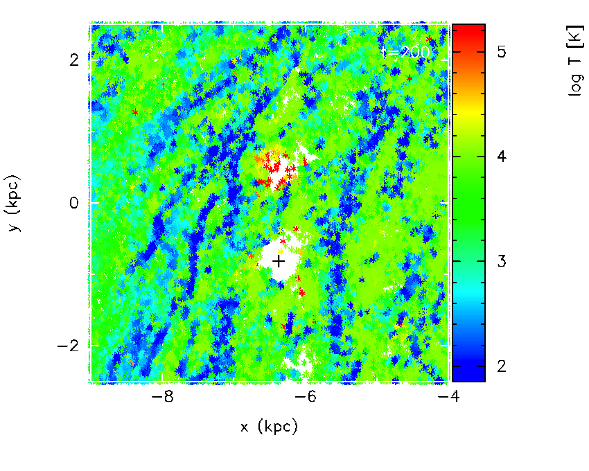
Figure 2: Particles are plotted for a subsection of Run L20 (with 20 per cent efficiency), specifically illustrating holes that have been blown out by supernovae. The region selected is indicated by the white box in Fig. 1. All the particles are plotted which lay between $z=-0.5$ and 0.5 kpc, their colour indicates the temperature.

4.1 Structure of the disc

We show the structure of the disc (including the spiral component of the potential) for efficiencies of 5, 10 and 20 per cent at a time of 200 Myr, and 1 per cent at a time of 125 Myr in Fig. 1. For the 1, 5 and 10 per cent cases, the 4-armed spiral structure is clear, but there is also a lot of substructure in the disc, and many filamentary interarm features, or spurs.

For the 1 per cent case, much of the gas becomes confined to dense, gravitationally bound clumps either in the spiral arms, or moving from the spiral arms into the interarm regions (see also Dobbs et al. 2011). As such, we are only able to run this calculation for a short time. Because the gas is gravitationally bound in these dense clouds, the elongated spurs seen in the other panels are unable to form as readily. The structure for the 5 and 10 per cent cases is similar to what we would expect to see in spiral galaxies – there are clear spiral arms and spurs. Thus the feedback does not prevent the formation of dense clouds of gas, nor the evolution of these clouds into spurs. For the 20 per cent efficiency case, feedback begins to dominate the structure of the disc. The arms are more broken up, and consequently it is more difficult to distinguish spiral arms from interarm substructure. The structure for the 40 per cent case is similar to that for 20 per cent, though the spiral arms are even less clear. The interarm spurs are clearest for the 5 per cent case.

In the 20 per cent efficiency case, there are many large holes in the disc, which have been blown out by supernovae. Such holes occur for all the $\epsilon>1$ per cent cases, but are less noticeable with lower efficiencies. It is also not so obvious to determine which features are holes blown out by supernovae, and which features are simply less dense regions between spurs or clouds which occur regardless of supernovae feedback (e.g. Dib & Burkert 2005; Dobbs & Bonnell 2006; Dobbs 2008). In Fig. 2 we show a subsection of the 20 per cent efficiency case (Run L20), corresponding to the box in Fig. 1. We plot the temperature of all particles for $|z|<0.5$ kpc in the region. The two holes in the centre, both several 100 pc across, are clearly associated with hot gas, and therefore supernovae feedback. The lower hole (as indicated by the cross) is particularly devoid of any particles.

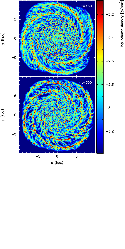
Figure 3: The gas column density is shown for the calculation using a star formation efficiency of 5 per cent (Run L5), at times of 150 and 300 Myr.

We show the structure of the disc for the 5 per cent efficiency calculation (Run L5) at times of 150 and 300 Myr in Fig. 3. At 150 Myr, the arms are slightly wider, and there is a smaller arm-interarm density contrast. At 300 Myr, there are a few more noticeable, and denser, clumps along the arms, but the structure is largely similar. For the highest star formation efficiency simulations the structure is more time dependent. As we will show in Section 4.5, the star formation rate peaks between 50 and 100 Myr. For the higher efficiency cases (Runs L20 and L40) this leads to substantial disruption of the gas disc (particularly for Run L40, where holes of a few kpcs across are produced) at earlier times.

4.2 The CNM, WNM and unstable regime

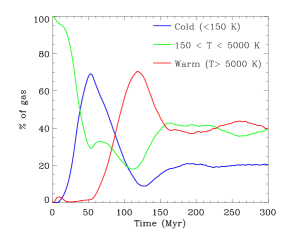
Figure 4: The fraction of gas in the cold, unstable and warm phases is shown versus time for Runs L5 and L20, the calculations with $\epsilon=$ 5 per cent (top), and 20 per cent (lower).

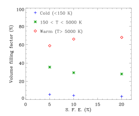
Figure 5: The volume filling factor for the cold, unstable and warm phases is plotted for the calculations with efficiencies of 5, 10 and 20 per cent (Runs L5, L10 and L20), at a time of 200 Myr.

The structure of the cold (i.e. $\sim 100$ K) and warm ($\sim 10^{4}$ K) phases of the ISM as shown in Fig. 2 is typical for these calculations. The cold gas is largely situated along the spiral arms and spurs, with the warmer gas filling in the regions between, thus similar to Dobbs et al. (2008). In the lower efficiency cases there is a little more cold gas, and the spiral arms are more continuous. The hotter gas (not included in Dobbs et al. 2008) is largely confined to supernovae bubbles and gas outside the plane of the disc.

In Fig. 4, we show the fraction (by mass) of gas in the cold, unstable and warm phases of the ISM. For the calculation with $\epsilon=$ 5 per cent, approximately one third of the gas lies in each phase. This is not dissimilar to observations and other simulations (e.g. Heiles & Troland 2003; Gazol et al. 2001; Kim et al. 2008). When $\epsilon=$ 20 per cent, only 20 per cent of the gas is in the cold phase, which is probably too low to reconcile with observations. We only obtained a high fraction of cold gas (65 per cent), similar to calculations without feedback (Dobbs, 2008) in the calculation with 1 per cent efficiency. There is some gas in the hot phase in these calculations but this constitutes very little mass, $\lesssim 1$ per cent of the total gas in the calculations with 5 and 10 per cent efficiency and a few per cent in the calculations with 20 and 40 per cent efficiency. For the 40 per cent efficiency case (Run L40), the majority of the gas (60–70 per cent) lies in the warm phase.

The volume filling factor for the different phases is shown in Fig. 5, for the calculations with 5, 10 and 20 per cent efficiency, at a time of 200 Myr. We calculate the filling factor for gas within a height of 1 kpc, and a radius of 10 kpc. There is little variation with efficiency, the warm and cold gas occupying slightly higher and lower volumes for higher star formation efficiencies. Volume filling factors are not well known for the ISM, though the filling factor of the CNM is believed to be 1 (Cox, 2005) or a few (McKee & Ostriker, 1977) per cent. The filling factor of the WNM is thought to be about 50 per cent (Heiles & Troland, 2003). Thus our estimates are in approximate agreement with the observations.

4.3 Velocity dispersion of the gas

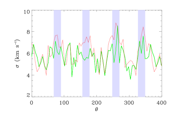
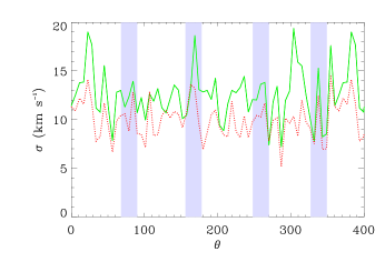
Figure 6: The velocity dispersion is calculated for an annulus of the disc for the 5 (left) and 20 (right) per cent efficiency calculations (Runs L5 and L20) at a time of 200 Myr. $\theta$ is the direction anticlockwise round the disc. The grey regions indicate the location of the spiral arms. The velocity dispersions, $\sigma_{r}$ (red, dotted) and $\sigma_{z}$ (green, solid) are between 4 and 8 km s^-1 when $\epsilon=$5 per cent, and between 6 and 20 km s^-1 when $\epsilon=$20 per cent.

Observations indicate that, with the exception of very hot gas, the velocity dispersion in the ISM is typically 5–10 km s^-1. In previous work without stellar feedback (Dobbs et al., 2006), we found that a velocity dispersion of this magnitude is achieved in the spiral arms, but quickly decays in the interarm regions. In Fig. 6, we show the velocity dispersion from an annulus of the disc, from the calculations with 5 (left) and 20 (right) per cent efficiencies (Runs L5 and L20), at a time of 200 Myr. We select particles within an annulus of width 1 kpc, a central radius of 7.5 kpc, and divide the annulus into 64 sections azimuthally. We show the velocity dispersion in the plane of the disc ($\sigma_{r}=\sigma(\sqrt{v_{x}^{2}+v_{y}^{2}}))$ and the vertical dispersion, $\sigma_{z}$.

We see from Fig. 6 that for the 5 per cent efficiency case (L5), there tend to be peaks in the velocity dispersion corresponding to the location of the spiral arms. The peaks are also higher for the velocity in the plane of the disc, whilst in the interarm regions, the velocity dispersions are similar in the two directions. However unlike Dobbs et al. (2006), the velocity dispersion is still maintained above 4 km s^-1 in the interarm regions. The enhancement of the velocity dispersion in the spiral arms is likely due to the higher star formation rate in the spiral arms, but the relatively higher increase for the dispersion in the plane of the disc suggests the spiral shock is also relevant. In contrast, the velocity dispersion for the 20 per cent efficiency case (Run L20), there is no correlation of the dispersion with the spiral arms. This is perhaps not surprising given that the spiral structure is weaker in this case. The velocity dispersion is observed to be higher in the spiral arms of NGC 0628 (Shostak & van der Kruit, 1984) and M51 (Hitschfeld et al. 2009, Fig. 11), but not NGC 1058 (Petric & Rupen, 2007), though the latter has a less prominent spiral structure. The mean ratio $\sigma_{z}/\sigma_{r}$ is 0.9 for the 5 per cent case, and 1.2 for the 20 per cent calculation. These values decrease if only gas close to the midplane is selected.

We find $\sigma_{r}$ and $\sigma_{v}$ take values of 4–8 km s^-1 when $\epsilon=5$ per cent ($\bar{\sigma_{z}}=5.7$ km s^-1), 5–16 km s^-1 when $\epsilon=10$ per cent ($\bar{\sigma_{z}}=9.1$ km s^-1) and 8–20 km s^-1 when $\epsilon=20$ per cent ($\bar{\sigma_{z}}=12.6$ km s^-1). Thus the velocity dispersions when $\epsilon=5-10$ per cent roughly match the observations, but are slightly high for $\epsilon=20$ per cent.

We also calculated the velocity dispersions in the cold, unstable and warm phases. For the $\epsilon=5$ per cent calculation, $\bar{\sigma_{z}}$ is 5.1, 6 and 7.3 km s^-1 for the cold, unstable and warm phases respectively. When $\epsilon=20$ per cent, $\bar{\sigma_{z}}$ is around 12 km s^-1 in the cold and unstable phases, and 20 km s^-1 in the warm phase. For Run L5, the ratio $\sigma_{z}/\sigma_{r}$ is lower for the cold gas, and there is a greater tendency for the $\sigma_{z}$ and $\sigma_{r}$ to coincide with the spiral arms for the cold gas. The latter behaviour is also seen in M51, when comparing HI and H₂, and in fact the peak HI dispersion is not at all coincident with the spiral arms (Hitschfeld et al., 2009).

In all cases, the velocity dispersions vary with time earlier in the calculations, following the variation in the star formation rate (see Section 4.5). The velocity dispersions are higher when the star formation rate is higher.

4.4 Scale heights of the gas

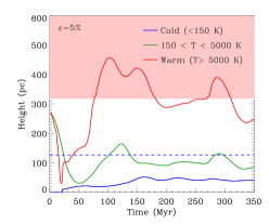
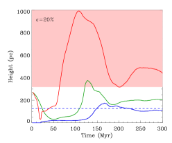
Figure 7: The scale heights of the cold, unstable and warm phases of the ISM are shown with time for the 5 (top), 10 (centre) and 20 (lower) per cent efficiency calculations (Runs L5, L10 and L20). The scale height of the warm gas can be between 325 pc and 1 kpc (red filled region), depending on whether the gas is ionised, whilst the scale height of the cold gas is estimated to be 127 pc (blue dashed line) (Cox, 2005).

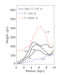
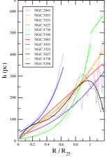
Figure 8: The scale height versus radius is shown for the calculations L5, L10 and L20 as indicated. The scale height is calculated from gas between 100 and $10^{5}$ K. Scale heights for the cold gas, and warm gas, from the 10 per cent efficiency calculation (Run L10) are shown separately as blue and red dashed lines. The right hand panel shows the scaleheight of neutral HI for a selection of early-type spiral galaxies (Bagetakos et al., 2011). The solid and dotted lines represent different techniques. In both simulations and observations the scale height is much lower in the inner regions of the disc.

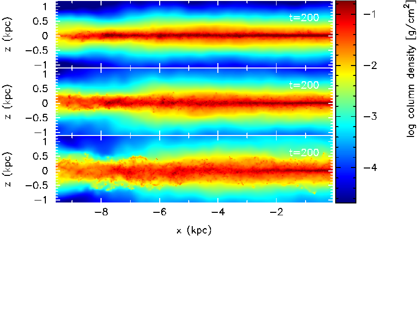
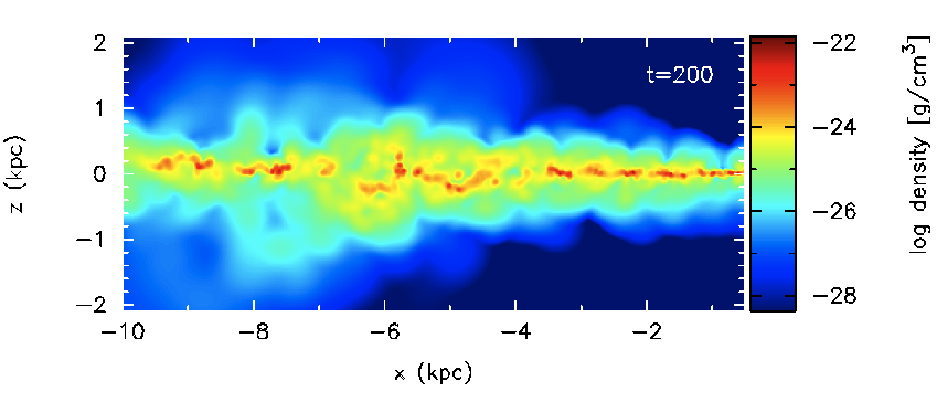
Figure 9: The column density in the vertical plane is shown (top panel) of the 5 (top-most), 10 (center) and 20 (third panel) per cent efficiency at time of 200 Myr. The column density is calculated by integrating along the direction of the $y$-axis. Without any feedback, the vertical extent is about half that of the 5 per cent (top) case, thus feedback is essential to reproduce the disc scale height. The lowest panel shows a cross section in the $zx$ plane for the 10 per cent efficiency case.

The fact that we find velocity dispersions of order 5–15 km s^-1 in these models suggests that we are reproducing the dynamics of the ISM reasonably well. The scale heights of the disc are then largely determined by the galactic potential we adopt.

In Fig. 7, we show the scale heights for the gas in the different phases of the ISM with time for the 5, 10 and 20 per cent calculations. As there is a substantial variation of scale height with radius, as shown in Fig. 8, we calculate the average scale height for gas only between radii of 5 and 10 kpc. The scale heights of the gas components suggested by Cox (2005) are 127 pc for the cold gas, and the warm gas can have heights between 325 pc and 1 kpc depending on whether the gas is ionised (see Fig. 7). From Fig. 7, the 20 per cent efficiency model appears to agree best with the observations for the cold gas. Though if we take a radius of 8 kpc, which is similar to the solar neighbourhood, the 10 per cent efficiency case best fits the observations, with the scale height of the cold gas around 100 pc (Fig. 8).

We also show in Fig. 8 the observed scale heights versus radius for neutral HI in nearby spiral galaxies, from the THINGS survey (Bagetakos et al., 2011). Both these and the simulations show an increase in the scale height with radius, from $<50$ pc to $>200$ pc, although our scale heights tend to flatten or decrease at the largest radii. The variation with radius in our simulations is predominantly due to the galactic potential we use.

We find an offset between the time supernovae first occur (around 40 Myr) and the increase in scale height for the different phases (Fig. 7). This offset is largest for the cold gas, where it is around 100 Myr. We interpret the offset for the warm gas as the time it takes for gas to leave the plane of the disc, i.e $z_{h}/c_{s}$ where $z_{h}$ is the scale height and $c_{s}$ is the sound speed. For the cold gas, we expect cumulative effects from star formation over a longer period of time are also required to increase the scale height.

We further illustrate the impact of supernovae on the vertical structure of the disc in Fig. 9. Before stellar feedback occurs, the gas is confined to a very narrow ($\lesssim 40$ pc) band in the mid-plane. For the 5 per cent efficiency case, gas is still fairly confined to the mid-plane, but the scale height is around double, and the material is less continuous in the mid plane. For the 20 per cent case, there is a lot more vertical structure in the gas. The lowest panel shows a cross section through the disc for the 10 per cent efficiency case after 200 Myr. Though we do not show the 5 and 20 per cent cases, for the 5 per cent case, the gas is more continuous in the midplane (which is actually more similar to the Canadian Galactic Plane (HI) Survey (Douglas et al., 2010)), whilst the 20 per cent case, there is more vertical structure.

Figure 10: The distribution of star formation events is displayed over a 20 Myr period (subtracting the phase of the potential) for the 5 (left) and 20 (right) per cent efficiency calculations (L5 and L20), in the plane of the disc (top), and out of the plane (lower).

As noted earlier, we would obtain different (and possibly higher) scale heights if we used a different potential. We also note that we do not include magnetic or cosmic ray pressure, which would increase the scale height of the warm components, and perhaps indirectly the cold gas. Neither do we allow for a warp which is present in our, and other galaxies. In addition, the scale height may not be the most useful measure of the vertical structure of the disc, for example if most of the gas is confined to the central midplane, whilst other clouds lie at far outside the midplane. Douglas et al. (2010) produced synthetic HI observations of gas from previous simulations. Similar synthetic HI maps, using the outcomes from the simulations presented here with feedback, may indicate better which of our models best reproduces the vertical structure of the HI in galaxies such as the Milky Way. Figs. 7, 8 and 9 however suggest we would obtain a much better agreement with the observations compared to the calculations without feedback shown in Douglas et al. (2010), where the gas was clearly too confined to the midplane.

4.5 Distribution and scale heights of supernovae

In Fig. 10 we display the locations of supernovae events over a 20 Myr period (from 180-200 Myr) for the calculations with 5 and 20 per cent efficiencies. The supernovae are concentrated to the spiral arms, especially for the 5 per cent case, as expected (McMillan & Ciardullo, 1996). The supernovae occupy a much larger vertical distribution for the 20 per cent case, compared to the 5. The scale heights of the supernovae events are 40 and 80 pc for the 5 and 20 per cent calculations respectively. This compares well to the distribution of OB stars, which are found to have scale heights of around 30–60 pc (Mihalas & Binney, 1981; Reed, 2000; Maíz-Apellániz, 2001; Urquhart et al., 2011). Scale heights of Type II supernovae are likely to be larger than those in our models (Ferrière, 2001), partly as the feedback is instantaneous, although estimates based on observations are also highly uncertain.

4.6 Star formation rates

Figure 11: The star formation rates are shown here versus time for the calculations with different efficiencies (Runs L5, L10 and L20). The star formation rate is not very steady, particularly at the early stages of the calculations. Simulations with higher efficiencies generally have higher star formation rates, but by 200 Myr the correspondence is less than linear, since with higher efficiencies the gas has higher velocity dispersions and less is in the cold, dense phase.

We show in Fig. 11 the star formation rate versus time for the calculations with different efficiencies. The star formation rate is not particularly steady for the duration of these calculations, particularly for the higher efficiency cases where the star formation rate is very high initially and then drops dramatically (see also Papadopoulos & Pelupessy 2010). As seen in Fig. 4, the gas in the disc initially cools, which leads to a high level of star formation. This then produces a large degree of warm gas, and correspondingly a large drop in the rate of star formation. The star formation rates then appear to show less dramatic changes with time. One can see that during the initial burst of star formation, the star formation rate scales with the efficiency. However at later (after 150 Myr) times, the star formation rates are much more similar regardless of the efficiency. This is because after the initial phase of star formation, the models with high efficiency have generated more hot gas and there is less material available for star formation, whereas the models with low efficiency have a higher fraction of cold, dense gas. The velocity dispersion of the gas is also higher in the higher efficiency cases (Section 4.4). So for example when $\epsilon=20$ per cent, the star formation rate is only around double that compared to when $\epsilon=5$ per cent at 200 Myr. At later times, the star formation rate for the 5 per cent efficiency case even exceeds that of the 10 per cent. As we will discuss in Section 7, this is due to a number of long-lived bound clouds (note that our calculations include short-lived unbound and bound clouds, but the long-lived clouds are by necessity bound). Such clouds are present only in calculations with low star formation efficiencies; with higher efficiencies the feedback is always sufficent to disrupt the cloud, and clouds are short-lived. Though not very numerous, these clouds have a disproportionate effect on the star formation rate and account for the continued increase in the star formation rate past 300 Myr for the 5 per cent efficiency calculation.

We show how the star formation rate varies with the global surface density, and how our results compare to the Schmidt-Kennicutt relation in Section 6, where we present different surface density calculations.

5 Results - Calculations with a non-spiral potential

In this section we investigate the importance of spiral density waves for star formation, and the structure and properties of the ISM. The calculations L5_nosp and L10_nosp are the same as the previous calculations L5 and L10 except the spiral component of the potential is not included. Thus they are very similar to calculations by Tasker & Tan (2009), and Wada et al. (2000), although the former did not include feedback and the latter were 2D.

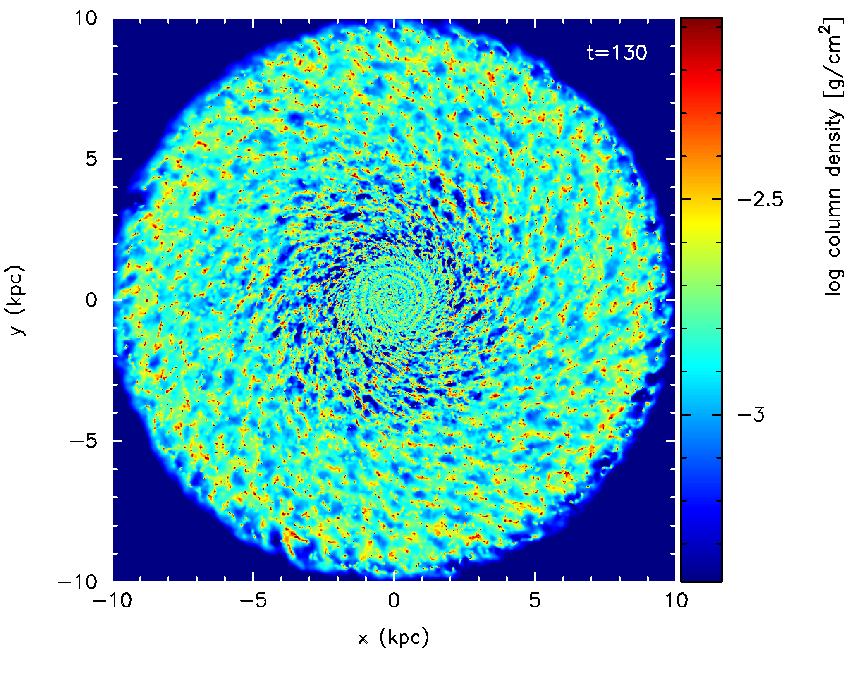
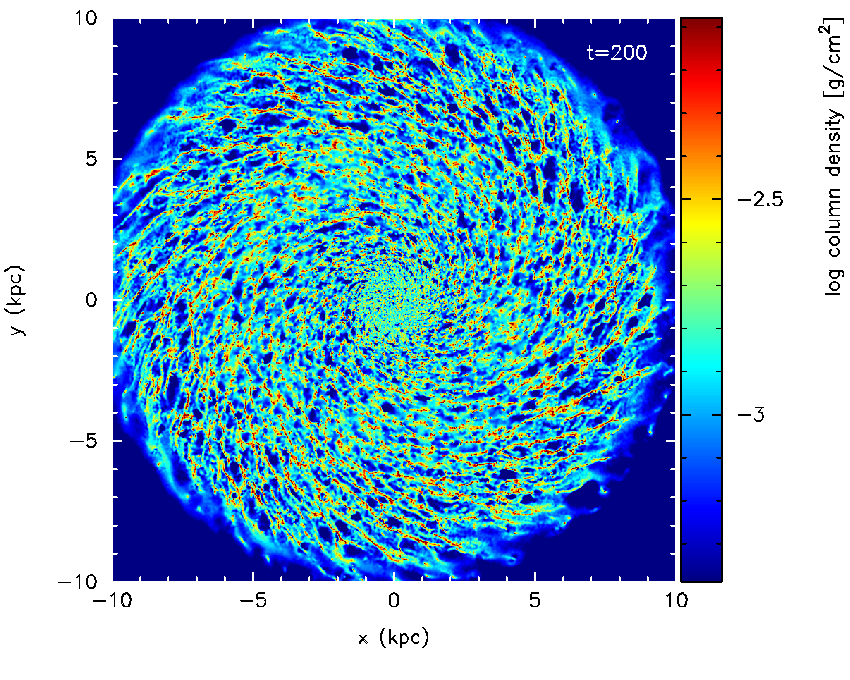
Figure 12: The column density is shown for Run L5_nosp, where $\epsilon=5$ per cent but there is no spiral component of the potential, at times of 130 and 200 Myr. At 130 Myr, the gas is much more diffuse (the amount of cold gas reaches a minimum at this point), and appears less structured, following a peak in the star formation rate. By 200 Myr, the structure is unchanging with time, and dominated by the cold dense gas. The evolution of Run L10_nosp is very similar. Many holes can be seen at 200 Myr due to supernovae, which appear more irregular and larger compared to those simply due to the flocculent structure.

We show the gas column density for the disc in Fig. 12. The gas is highly structured, consisting of very many small spiral arm segments. This is a somewhat simplified model since we adopt a completely smooth disc potential. Very few flocculent galaxies exhibit so much structure, though NGC 2841 is one possible example. Typically galaxies are susceptible to gravitational perturbations in the stellar disc, which lead to long, multiple arms in the gas and stars simultaneously (e.g. Dobbs & Bonnell 2007). Fig. 12 indicates however that the structure in the absence of a spiral density wave is probably similar to the interarm structure in the previous calculations with a spiral potential (e.g. Fig. 1). However the spiral arms in the models shown in Fig. 1 gather the gas together, and determine the spatial distribution of spurs.

5.1 Properties of the ISM

The scale heights, and amount of gas in the WNM tend to be slightly higher in Run L5_nosp compared to Run L5 (by $\sim$10–20 per cent), indicating the supernovae are having a greater impact on the ISM. This is probably because the gas is not gathered into spiral arms, so the hot gas can more readily diffuse, and survive in the lower density regions. Otherwise, the distributions of the cold, unstable and warm phases of the ISM in the models without a spiral component are largely similar to those shown earlier with a spiral density wave (Figs 4, 5, 6), and likewise the scaleheights of supernovae events (Fig. 9). Hence we do not show these results for the non-spiral models. The main difference in the calculations with and without the spiral potential, is that with a spiral potential, the gas is gathered into more massive clouds in the spiral arms (see Section 7).

5.2 Star formation rates

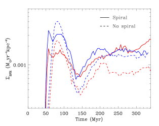
Figure 13: The star formation rate is plotted versus time for galaxies with and without a spiral potential. The red lines indicate the 5 per cent efficiency calculations (Runs L5 and L5_nosp), whilst the blue lines indicate the 10 per cent efficiency calculations (Runs L10 and L10_nosp). When $\epsilon=$5 per cent, the star formation is typically higher by factor of 2 or so with the spiral component of the potential. The difference is partly due to the presence of a few massive, bound, long-lived clouds in the case with a spiral potential. When $\epsilon=$10 per cent, by 200 Myr the star formation rates are similar, regardless of the presence of the spiral component of the potential.

As discussed in the introduction, an important question is whether spiral formation drives the triggering of star formation. In Fig. 13 we show the star formation rate for Runs L5, L5_nosp, L10 and L10_nosp versus time, thus comparing the star formation rate with and without the spiral component of the potential. For the 5 per cent efficiency calculations (Runs L5 and L5_nosp), the star formation rate in the calculation with a spiral component is 2–2.5 times higher than without. For the 10 per cent cases, the calculations evolve to very similar star formation rates. With the lower efficiency, the spiral arms are able to gather material into more massive clouds and by the end of the calculation, there are several long-lived, bound, massive clouds (Section 7). These clouds have a disproportionate effect on the star formation rate. In contrast, for the 10 per cent efficiency case, such clouds do not form regardless of the presence of spiral shocks, so there is less difference in the star formation rate.

The presence and strength of the spiral potential also determines when star formation begins in the calculation. There is a higher initial star formation rate without a spiral potential - possibly because star formation commences everywhere in the galaxy simultaneously, rather than starting in the spiral arms.

6 Results - Different surface density calculations

6.1 Structure and properties of the ISM

In Fig. 14 we show the column density distribution for Run M10, which has a higher surface density of 16 M_⊙ pc^-2, and an efficiency of 10 per cent. The structure of the disc is fairly similar to Run L10, with fairly continuous spiral arms, and clear spurs. The arms also appear slightly wider than the lower surface density case.

For the calculation with an efficiency of only 5 per cent, we obtained more massive clouds along the spiral arms. We include a section of the disc, showing these massive clumps, in Fig. 15. Similarly to Run L1, we cannot run this calculation further as the density of the gas becomes very high in these massive, strongly bound and long–lived clouds. However we do note that the similarity between the structure along the arm and simulations by Shetty & Ostriker (2006). In both cases, the formation of the massive clouds is likely due to gravitational instabilities rather than cloud collisions. Consequently the spiral arms are not so continuous, the gas being instead arranged into disproportionately massive clouds. In Shetty & Ostriker (2006) these clouds were stabilised by magnetic fields, which we do not include, and a temperature floor of $10^{4}$ K.

Unlike Run M5, for the case with a higher efficiency (M10), the feedback is sufficient to prevent the formation of very strongly bound clouds, thus the continuous gas spiral arms are maintained. Thus perhaps rather counterintuitively the higher level of feedback helps maintain the spiral structure in the gas.

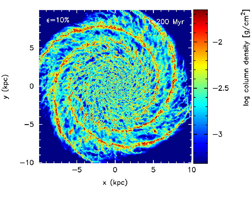
Figure 14: The column density is shown for Run M10, with a higher surface density of 16 M_⊙ pc^-2, and where $\epsilon=10$ per cent. The structure is fairly similar to the lower surface density model with $\epsilon=10$ per cent (Figure 1).

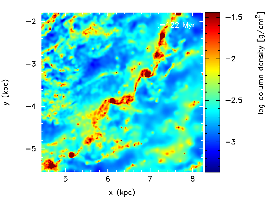
Figure 15: The column density is shown for a section of Run M5, at a time of 122 Myr. The figure shows the organisation of gas into dense discrete clumps along the arms, whilst continuous spiral arms cannot be maintained.

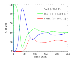
Figure 16: The fractions of gas (by mass) in the cold, unstable and warm regimes for the calculation with $\Sigma=16$ M_⊙ pc^-2 and $\epsilon=5$ per cent (Run M10). The fractions of gas in the different phases is similar to those in the lower surface density models, but with slightly more cold gas.

In Fig. 16 we show the fraction of gas in different phases of the ISM with time for Run M10, with $\Sigma=16$ M_⊙ pc^-2. The fractions of gas in the cold, unstable and warm phases are similar to the lower surface density calculations. There is slightly more cold gas than the equivalent 8 M_⊙ pc^-2 calculation (Run L10), as expected for higher densities. The scale heights, and velocity dispersions are slightly higher (by around 25 per cent) in the intermediate compared to low surface density calculations.

6.2 Star formation rates

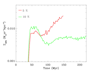
Figure 17: The star formation rates are shown from calculations M5 and M10, with a surface density of $\Sigma=16$ M_⊙ pc^-2. The star formation rate with a 5 per cent star formation efficiency actually becomes higher than than with 10 per cent efficiency because of the presence of long lived, massive, bound clouds, which form stars continuously over a long time period.

In Fig. 17 we show the star formation rate in Runs M5 and M10 (where $\Sigma=16$ M_⊙ pc^-2 and the star formation efficiency is 5 and 10 per cent respectively). For the 10 per cent efficiency case, the evolution of the star formation rate is more similar to the low surface density calculations; the star formation rate is initially high, then decreases, and stays at a more or less constant level. With 5 per cent efficiency, the star formation rate increases instead, and is actually higher than for the 10 per cent case. Again this is because in the 5 per cent efficiency case, there are massive, bound, long lived clouds, which have a marked effect on the star formation rate.

The star formation in Run M5 does not converge in our models. In reality, the lifetime of clouds in Run M5 would be regulated by the conversion of gas to stars, but we do not include this in our models. We found that the formation of strongly bound clouds which are not disrupted, tends to occur at lower efficiencies for higher surface density (40 M_⊙ pc^-2) calculations. Whilst this trend is probably correct, we do not have the same mass resolution in the high surface density calculations as the low surface density calculations, so cannot make a true comparison.

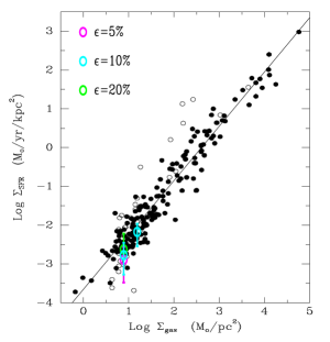
Figure 18: The star formation rates from the simulations with the spiral potential (Runs L5, L10, L20, M10) are plotted against surface density, the colours indicating the star formation efficiency. These points are plotted on Figure 2 from Kennicutt (2008). Filled circles denote luminous spirals an irregular galaxies with $M_{B}<−17$, and open circles show fainter dwarf irregular galaxies. The error bars indicate the range of the star formation rate over the duration the disc is forming stars. The non-spiral calculations are not included, but would lie roughly on top of the points shown here.

6.3 The Schmidt-Kennicutt relation

In this section we compare the star formation rate with the observed rates for galaxies, noting again that we do not include any a priori assumptions based on observations in order to determine the star formation rate. Observationally there is a clear trend, the Schmidt-Kennicutt relation (Schmidt, 1959; Kennicutt, 1998), between the star formation rate and the gas surface density. In Fig. 18 we show the star formation rate versus the total gas surface density, for Runs L5, L10, L20, and M10, where the star formation rate has converged. All include the spiral component of the potential. We can only estimate the star formation rates from the calculations, as they tend to be highly time dependent. So we show the star formation rate at 200 Myr, whilst the error bars indicate the maximum and minimum values of the star formation rate over the duration of the simulations.

Generally the star formation rates in our models provide reasonable agreement with observations. Although for the low surface density calculations, these points lie where the Schmidt-Kennicutt relation starts to turn over and there is a large degree of spread, so it is more difficult to compare with observations. We see however that the efficiency does not strongly affect the spread in the star formation rate. Furthermore, though for clarity we do not show the calculations without a spiral component, these points would lie on top of those already plotted. Thus we obtain a greater degree of spread simply from the time evolution of the galaxy, and whether the galaxy contains long-lived clouds, than the efficiency or presence of an imposed spiral pattern.

7 Properties of clouds

In Dobbs et al. (2011) we focused on the virial parameters of the molecular clouds formed in the simulations, and also discussed their aspect ratios. We found that with a star formation efficiency of 5 or 10 per cent, most of the clouds exhibited $\alpha>1$. With an efficiency of 1 per cent, most of the clouds had values of $\alpha<1$, and many had an aspect ratio of $\sim 1$, in disagreement with observations. In this section we give a broader perspective of the properties of the clouds. We show properties from all the calculations except M5, which does not show convergence. Although Run L1 also does not show convergence, we retain this as a comparison to show cloud properties when feedback is minimal. We select clouds as described in Dobbs et al. (2011).

7.1 Masses and virial parameters of the clouds

In Fig. 19 we plot the mass versus radius, and the distribution of virial parameters for calculations L1 (after 125 Myr), L5, L10, L5_nosp and M10 (at times of 200 Myr). These are the low surface density calculations with 1, 5 and 10 per cent star formation efficiencies, the $\Sigma=16$ M_⊙ pc^-2 calculation with $\epsilon=10$ per cent, and the simulation with no spiral potential and $\epsilon=5$ per cent. The virial parameters are calculated as described in Dobbs et al. (2011), where we aimed to match observational determinations of $\alpha$ . For model L5, we find one third of the clouds have $\alpha<1$ (by number, or 36% by mass), one third are marginally bound with $1<\alpha<2$, and one third are unbound with $\alpha>2$. We note that we omit thermal and magnetic energy, which would increase $\alpha$. We also did not include external pressure, though this does not readily lead to clouds in virial equilibrium (Field et al., 2011).

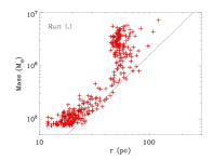
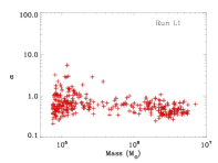
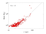
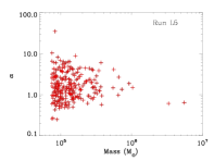
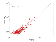
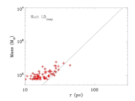
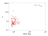
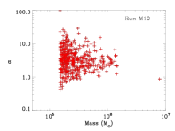
Figure 19: The masses and radii of the clouds are plotted (left), whilst their virial parameters are indicated on the right. The panels (in descending order) show the 8 M_⊙ pc^-2 surface density calculations with 1, 5 and 10 per cent efficiency, the calculation with no spiral potential and 5 per cent efficiency, and the calculation with 16 M_⊙ pc^-2 and 10 per cent efficiency. The low efficiency cases, and higher surface density calculations exhibit clouds which are disproportionately massive, and strongly gravitationally bound. The dotted lines indicate a constant surface density of 50 M_⊙ pc^-2.

From Fig. 19, we see that the clouds in a given galaxy model generally exhibit similar surface densities, with little spread in the mass versus radius. The exception is the low efficiency model L1 ($\epsilon=1$ per cent), where there are overly dense clouds. In this case, where there is minimal feedback, the clouds can continue to increase in mass without being disrupted. These clouds also exhibit low virial parameters, and have long lifetimes. There are a couple of such massive clouds in Run L5. By 350 Myr in L5, these 2 clouds exceed $10^{7}$ M${\odot}$ whilst several more long-lived bound, massive, clouds have also formed.

The departure of the clouds from constant surface densities is likely related to the Jeans mass for a thin disc, $M_{J}=c_{s}^{4}/G^{2}\Sigma$, where $c_{s}$ is the sound speed and $\Sigma$ is the surface density. Taking instead of the sound speed, a velocity dispersion $\sigma\sim 7$ km s^-1 for model L5, and a surface density of 50 M_⊙ pc², gives $M_{J}=2.4\times 10^{6}$M_⊙. Thus clouds above this mass are not supported by the velocity dispersion against global gravitational perturbations. This is only an approximate estimate, especially since the velocity dispersions are not equivalent to an isotropic sound speed, however this value fits almost exactly with the turnover in Figure 19 (second panel) The turnover for the 1 per cent calculation also appears to be at lower masses which corresponds to slightly lower velocity dispersions in that calculation. If we changed the criteria for selecting clumps (and thereby $\Sigma$ above), we would change the mass where this turnover occurs accordingly.

The second and fourth panels in Fig. 19 compare calculations with and without the spiral component of the potential (Runs L5 and L5_nosp). There is a clear cut off at $3\times 10^{5}$ M_⊙ for the clouds from the calculation with no spiral potential. Even for masses below $3\times 10^{5}$ M_⊙, there are significantly fewer clouds in the run with no spiral potential. Thus the spiral density wave is vital for gathering gas together to produce larger clouds. Though we have only a relatively small sample of galaxies, observations also seem to indicate that molecular clouds are less massive in galaxies without a strong spiral pattern, e.g. M33 (Rosolowsky et al., 2003). For both the 10 and 20 per cent efficiency cases, the masses of the clouds exceed those in the calculation with no spiral potential.

Though we caution there are only a small number of clouds found in Run L5_nosp, and these clouds are not well resolved, we found that there are a higher fraction of bound clouds. With no spiral potential 70 per cent of the clouds are bound compared to only 30 per cent with the spiral potential (even when just considering the lower mass clouds). In other respects the clouds are similar. The distributions of aspect ratios are similar, and the clouds in Run L5_nosp are short-lived. This difference in $\alpha$ could reflect that the spiral potential allows gas to be gathered together independently of gravity, whereas without the spiral potential, the clouds are more often formed bound, undergo gravitational collapse, and are then dispersed.

The third and fifth panels compare the properties of clouds in models with different surface densities (L10 and M10, with 8 and 16 M_⊙ pc^-2 and $\epsilon=10$ per cent). The properties of the clouds are similar. There is a greater difference between models L5 and M5 (as likewise between L1 and L5), but M5 does not show convergence.

We compute mass spectra for the calculations with different star formation efficiencies in Fig. 20 (Runs L1, L5 and L20). The cloud mass function has a slope of around $dN/dM\propto M^{-1.9\pm 0.1}$ for the clouds in Runs L5 and L20, with 5 and 20 per cent efficiencies (and though not shown, the slope is similar for Run L10 with 10 per cent efficiency). This is similar to the results we obtained in Dobbs (2008), and to observations (Heyer et al., 2001). Thus the star formation efficiency does not change the slope, rather the level of stellar feedback determines the normalisation of the cloud mass function. For the calculation with 20 per cent efficiency, there are fewer clouds, and the maximum mass is $7.5\times 10^{5}$ M_⊙. Though we do not show it in Fig. 20, the cloud mass spectrum for Run M10, with a higher surface density, has a slightly shallower slope ($dN/dM\propto M^{-1.65\pm 0.1}$), which could be due to the increased importance of self gravity (Dobbs, 2008; Dib et al., 2008). The normalisation is also naturally higher.

The mass function for Run L1, with $\epsilon=1$ per cent is very different. There is a peak at $5\times 10^{6}$ M_⊙, which is not seen in observations. Again these high mass clouds are gravitationally bound, long lived clouds. In Run L1, feedback is insufficient to disrupt the clouds, therefore they can continue to increase in size. Their mass is instead only limited by their age, and the accretion of gas from the surrounding medium. In fact any of the simulations where we find a significant number of clouds which do not follow a constant surface density relation (i.e. L1, eventually L5, and M5) would exhibit such a bimodal distribution.

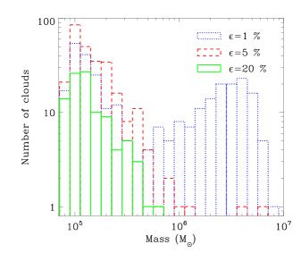
Figure 20: The mass spectra are shown for the calculations with $\epsilon=1,5$ and 20 per cent (L1, L5 and L20), where there is a spiral potential. The spectra are calculated at a time of 200 Myr for Runs A5 and A20, and 125 Myr for Run A1. The slope of the mass spectra is about $dN/dM\propto M^{-1.9\pm 0.1}$ when $\epsilon=5$ and 20 per cent, the mass spectrum is merely shifted to lower masses with the higher star formation efficiency. The spectra for the 1 per cent efficiency case (Run L1) exhibits a bimodal distribution due to a population of long-lived bound clouds.

7.2 Cloud heights and Orion

Earlier in Fig. 9 we showed the heights of supernovae events in the disc. We also determined the height of the clouds found in calculations L5, L10 and L20, at a time of 200 Myr. The maximum heights of the clouds are $\sim$ 120, 220 and 300 pc for the calculations with 5, 10 and 20 per cent efficiency respectively. Orion lies at a height of 200 pc above the midplane. For the 10 and 20 per cent efficiency calculations, clouds with heights similar to Orion are relatively easy to produce. For the 5 per cent calculation, they are much rarer. Fig. 9 shows that a small number of supernovae have occured at heights of 200 pc, suggesting we would only find such a high latitude cloud at particular time intervals. The scale heights are similar or higher for the higher surface density calculations.

7.3 Cloud rotation

The angular momenta of the clouds is shown in Fig. 21 for Run L5. As pointed out in Dobbs (2008), cloud collisions can be sufficiently disruptive to cause GMCs to have a net rotation in a direction opposite to the rotation of the galaxy. The distribution is similar to that shown in Dobbs (2008), with a similar fraction (37 per cent) of retrograde rotating clouds. The low mass clouds have slightly higher angular momenta compared to Dobbs (2008). The distribution of angular momenta is similar for Run M10, though with a few more higher momentum clouds.

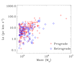
Figure 21: The angular momenta are shown for clouds from Run L5 ($\epsilon=5$ per cent) at a time of 200 Myr. Nearly 40 per cent of the clouds exhibit retrograde rotation, though the 2 very massive clouds, long-lived clouds are prograde.

We show the fraction of retrograde clouds for the different calculations in Fig. 22. Observations of clouds in our Galaxy, and M33, suggest that $\sim 40$–60 per cent of clouds exhibit retrograde rotation (Phillips, 1999; Rosolowsky et al., 2003; Imara et al., 2011; Imara & Blitz, 2011). For the calculations with $\epsilon=$ 5, 10 and 20 per cent (L5, L10 and L20), and the medium surface density calculation with $\epsilon=$ 10 per cent (M10), the fraction of retrograde clouds agrees with observations. For Run L1 ($\epsilon=1$ per cent) however, there are only $\sim 13$ per cent retrograde clouds, much lower then observations. In this calculation, much of the gas accumulates into $>10^{6}$M_⊙ clouds which rarely collide and are not substantially disrupted by stellar feedback. Thus there is no mechanism to cause these clouds to rotate retrogradely. Instead the clouds continue to accrete gas due to self gravity.

We also show in Fig. 22 the fraction of retrograde clouds for Runs L5_nosp and L10_nosp. In both cases the fraction of retrograde clouds is less than with the spiral potential. This again points to a scenario where collisions are less important in the calculations without a spiral potential, and the clouds mainly form by self gravity.

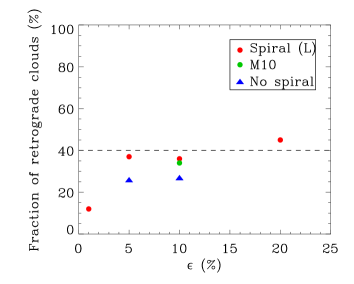
Figure 22: The fraction of retrograde clouds is shown versus star formation efficiency for the models L1, L5, L10, L20, M10, L5_nosp, and L10_nosp. The dashed line shows the fraction of retrograde clouds estimated for M33 (Rosolowsky et al., 2003). The fraction of retrograde clouds matches observations for the spiral calculations, with the exception of the $\epsilon=1$ per cent case, whilst the fraction is a little low without a spiral potential.

8 Conclusions

In order to model the ISM in spiral galaxies we have carried out numerical three-dimensional hydrodynamic simulations of gas flowing in a fixed, full disc, global potential. The model involves a standard cooling law, and heating from background UV radiation together with localised input from star-formation episodes. Star formation is assumed to occur instantaneously when a parcel of the ISM becomes sufficiently compact and self-gravitating that it undergoes dynamical collapse. When this occurs a fraction, $\epsilon$, of this gas is assumed to form stars and to provide instantaneous feedback to the ISM. Using these simple ideas we are able to reproduce the following features of the ISM:

8.1 Gas properties

1. We obtain roughly equal fractions of gas which are in the cold ($T<150K$), intermediate, thermally unstable ($150K<T<5000K$) and warm ($T>5000K$) phases. The relative fractions depend mainly on the assumed efficiency $\epsilon$ of star- formation feedback (Figure 4).

2. The scaleheights of the cold, unstable and warm phases are in reasonable agreement with observations. Here values of $\epsilon$ in the range 0.1 – 0.2 give the best fit to the observations of the Galaxy (Figure 7), as well as for a number of external early-type spirals (Figure 8).

3. The velocity dispersion both in the plane, $\sigma_{r}$, and perpendicular to it, $\sigma_{z}$ are similar to the observed velocity dispersions. Values obtained range from an average of around 6 km s^-1 for $\epsilon$ = 0.05 to around 12 km s^-1 for $\epsilon$ = 0.2 (Figure 5). For the smaller values of $\epsilon$ we find that $\sigma_{r}\approx\sigma_{z}$ , and note that values in the interarm regions are marginally smaller ($\approx$ 5 km s^-1) than in the arms ($\approx$ 7 km s^-1). For the higher values there is little arm/interarm dependence, but there is then a slight trend for $\sigma_{z}$ to be on average larger than $\sigma_{r}.$

8.2 Molecular cloud properties

1. The mass spectra of clouds are of the form $dN/dM\propto M^{−1.9\pm 0.1}$ for values of $\epsilon$ in the range $0.05\leq\epsilon\leq 0.2$, with the masses being shifted to lower values for the higher values of $\epsilon$ (Figure 20).

2. The range of values of the $\alpha$ parameter which describes the degree to which the clouds are bound (see also Dobbs et al. 2011). For a surface density of $\Sigma=8M_{\odot}$ pc^-2, and for values of $\epsilon$ in the range $\epsilon=$ 0.05 – 0.2 it is found that most clouds are unbound, or marginally bound, and have $\alpha$ in the range $\alpha\approx$ 1.0 – 10. For smaller values of $\epsilon$ the models produce clouds which are disproportionately massive and strongly gravitationally bound. Higher surface density discs also tend to show more bound clouds for equivalent values of $\epsilon$.

3. If molecular clouds formed simply by gravitational collapse from the ISM then conservation of angular momentum acquired from the galactic shear would ensure that they all rotate in the prograde direction. In fact, both in the Galaxy and in M33 about 40 per cent of clouds rotate in the retrograde direction. As we have remarked before (Dobbs, 2008), if clouds build predominantly by collisional build-up of dense structures within an already inhomogeneous ISM, then the tendency of clouds to display both prograde and retrograde rotations in almost equal measure can be explained. We confirm this result in the current simulations (Figures 21 and 22). In Figure 22 we note that for the models with no spiral structure, in which the clouds build preferentially by self-gravity rather than collisions, the fraction of retrograde clouds is significantly reduced.

8.3 Star formation

1. After initial transient behaviour, we find for $\epsilon\approx$ 0.05–0.2 that global star formation rates settle down to equilibrium values (Figures 11, 13 and 17) which depend on the average galactic gas surface density in agreement with the observed findings of Kennicutt (2008) (Figure 18). This result is independent of the presence or absence of an imposed spiral potential (cf. Dobbs & Pringle 2009). For efficiencies of $\epsilon\lesssim 0.5$ we find that the spiral potential gives rise to long-lived, massive, bound clouds in which star formation continues to accelerate over a long period; for these calculations we are unable to determine an equlibrium star formation rate.

2. We find that for an imposed spiral potential the distance from the galactic plane where star formation occurs depends significantly on the assumed value of $\epsilon$ (Figure 9). For the lower value of $\epsilon=0.05$ the star formation events occur with a scaleheight of 40 pc and do not stray more than around 150 pc above and below the galactic plane. In contrast, for $\epsilon=0.2$ the scaleheight of star formation events is around 80 pc, and events can occur up to around 500 pc from the plane.

In addition to these properties, we also obtain notable disagreements with the observations when there is little or no feedback, as exemplified by our calculation where $\epsilon=$ 0.01. In this case, the mass spectrum is bimodal, there are very few retrograde clouds, whilst the scale height of the ISM is too low in the absence of feedback.

9 Discussion

We have used an imposed potential to simulate galaxies with strong spiral structure resulting from tidal interactions or central bars in which the ISM is subject to strong shocks as it orbits in the galaxy. In such galaxies, the ISM flows through the azimuthal inhomogeneities in the galactic potential (spiral arms) and so we might expect molecular clouds to form mainly by collisional processes. We have not however examined galaxies where self-gravity of the stellar component provides the dominant azimuthal component of the potential – so called flocculent galaxies (Li et al., 2005; Clarke & Gittins, 2006; Dobbs & Bonnell, 2008; Fujii et al., 2011). In this case the inhomogeneities occur close to co-rotation and so the relative velocity of the gas in the spiral perturbations is strongly reduced. In such a scenario, we would not necessarily expect to find the same properties of GMCs. For example, we may well expect more prograde clouds compared to tidally (or bar) driven spirals. In such galaxies, the clouds are likely to form and disperse on timescales similar to the arm formation. A further question is whether the formation of massive GMCs has any influence on the stellar perturbations in the disc. We will address these issues in future calculations which consistently model flocculent spiral structure (see also Wada et al. 2011).

The main other work which has investigated cloud properties is Tasker (2011) and Tasker & Tan (2009). One main difference between those papers and the current work is that Tasker (2011) finds the majority of molecular clouds have $\alpha<1$. Tasker (2011) however does not include supernovae feedback (nor a spiral potential), which by comparing Runs L1 and L5 for example, is necessary to produce a population of unbound clouds. Instead Tasker (2011) adopts a temperature minimum, which presumably prevents runaway gravitational collapse. Tasker (2011) also finds slightly lower fractions of retrograde rotating clouds. This however is in agreement with our predictions that there are fewer retrograde clouds in the absence of a spiral potential, and that the fraction of retrograde clouds decreases with a less clumpy medium (Tasker 2011 compares calculations with and without a diffuse heating term). Both sets of calculations (see also Dobbs et al. 2011) find that clouds are relatively short-lived, i.e. $\lesssim 20$ Myr.

In our calculations, we observe the formation of large, massive clouds which are not readily dispersed. They occur when a low amount of energy is deposited as feedback, and are more frequent for discs with higher surface densities. Such clouds would be likely to form massive star clusters. Though they studied radiation pressure, rather than the implicit momentum and thermal feedback we include here, Krumholz & Dekel (2010) also found that below a certain star formation efficiency (per free fall time), clouds were not disrupted. Swinbank et al. (2010) compare clouds in the Local Group, the nearby ULIRG Arp220 and the z=2 sub-millimetre galaxy SMMJ2135-0102. Interestingly they find that the clouds in the interacting galaxy (Arp220) and the z=2 galaxy are much more luminous for their physical size compared to local Group counterparts. The massive clouds in our models also display higher, and prolonged amounts of star formation. Although from our calculations, the formation of such clouds is found to be dependent on the efficiency, surface density and presence of spiral struture, we caution that our models may be too simplified (e.g. no magnetic fields, no time-dependent stellar feedback), whilst higher density calculations are not so well resolved, to make firm predictions. Future work will involve models with more detailed stellar feedback, possibly in individual clouds, as well as more realistic models of galaxies where massive clouds are common, such as starburst and high redshift galaxies. Such calculations may also indicate differences in the star formation efficiency, as measured by the total mass of a given cloud converted into stars, and the Schmidt Kennicutt relation, in different environments.

10 Acknowledgments

The calculations presented in this paper were primarily performed on the HLRB-II: SGI Altix 4700 supercomputer and the Linux cluster at the Leibniz supercomputer centre, Garching. Many of the images were produced using SPLASH (Price, 2007), a visualization tool for SPH that is publicly available at http://www.astro.ex.ac.uk/people/dprice/splash. CLD thanks Ian Bonnell for helpful discussions. We also thank an anonymous referee for suggestions which improved the paper.

Appendix A Supernovae feedback

We add feedback according to the snowplough solution for a Sedov blast wave test. The radius, velocity and temperature of the supernova bubble at a time $t$ (in years) are

$$R_{s}=1.13E_{51}^{115/511}n_{0}^{-135/511}t^{2/7}$$ (2)

where $E_{51}$ is the supernovae energy in units of $10^{51}$ ergs and $n_{0}$ is the ambient density in units of 1 cm^-3,

$$T_{s}=2.82\times 10^{8}E_{51}^{134/511}n_{0}^{-24/511}t^{-4/7}$$ (3)

and

$$V_{s}=413n_{0}^{1/7}\zeta_{m}^{3/4}E_{51}^{1/14}(4/3t_{*}-1/3)^{-7/10},$$ (4)

where

$$t_{*}=t/t_{PDS};\;t_{PDS}=\frac{3.61\times 10^{4}}{e}\frac{E_{51}^{3/14}}{\zeta_{m}^{5/14}n_{0}^{4/7}}yr,$$ (5)

$e$ is the natural logarithm and $\zeta_{m}$ is a metallicity factor set to unity. These equations are taken from (Ikeuchi et al., 1984) ($R_{s}$ and $T_{s}$) and (Cioffi et al., 1988) ($V_{s}$). The expressions from Ikeuchi et al. (1984) utilise analytic calculations for blast waves from a number of sources (Sedov, 1959; Woltjer, 1972; Chevalier, 1974; McKee & Cowie, 1977; McKee & Ostriker, 1977).

Our calculations provide $E_{51}$ (from Eqn. 1), $R_{s}$, the radius of the region of gas and $n_{0}$, the ambient density (calculated from a 50 pc width ring of gas surrounding the region where feedback is inserted). We therefore rearrange Eqn. A1 to find $t$, which we then insert into equations A2 and A3 to find the temperature and velocity. The values of $t$ are typically $10^{4}-10^{5}$ years and therefore slightly higher than the time at which the transition from the Sedov to snowplough solution occurs.

We initially performed simulations of a single energy deposit in a 1 kpc cubed box. We found good agreement with the analytic results provided the SPH timesteps were not too large and the energy is not deposited in a tiny number of particles. Interparticle penetration becomes problematic for long timesteps (see also Saitoh et al. 2008), but we found this only occurred with timesteps of $10^{6}$ years. In our global simulations, the largest global timestep is much smaller than this. We also chose the radii of the regions to insert supernovae so that there are typically a few 10’s of particles within those regions.

Appendix B Numerical tests

Using our adopted implementation of feedback, we do not add star or sink particles, rather we simply insert energy above a certain density criterion. With a mass resolution of 2500 or 5000 M_⊙, we do not resolve the Jeans length at this criterion (though we note that i) the densities of the particles in the molecular clouds are typically one or two orders of magnitude below our feedback threshold, and ii) the velocity dispersions are significantly higher than the thermal sound speeds). We did however test the dependence of our results on the criteria chosen, as well as adopting a temperature floor of 500 K.

In Fig. B1 we show the structure of the disc with density crtieria of 100, $10^{4}$ cm^-3, and a temperature floor of 500 K as well as a low resolution calculation with 250,000 particles. The structure of the disc is similar with the different density criteria. Though with the low density criterion, there is less molecular gas so there is slightly less feedback, and more bound clouds, giving an evolution more similar to Run L1. The global structure of the disc is also similar with the temperature floor, and the lower resolution, but the small scale structure is not captured.

We also checked the cloud properties in these (1 million particle) calculations. The clouds in the model with the very high density criterion are very similar compared to the clouds in L5. The mass spectrum (though with a slightly lower normalisation) has the same slope, and the distribution of angular momenta are very similar. For the model with the lower threshold, there are more bound clouds, and a smaller fraction of retrograde clouds. However this is to be expected given that the efficiency is effectively less in this calculation. For the calculation with a temperature floor of 500 K, the mass spectrum is shallower, probably since there is less small scale structure. There are also fewer (27 per cent) retrograde clouds, again presumably because the gas is less clumpy.

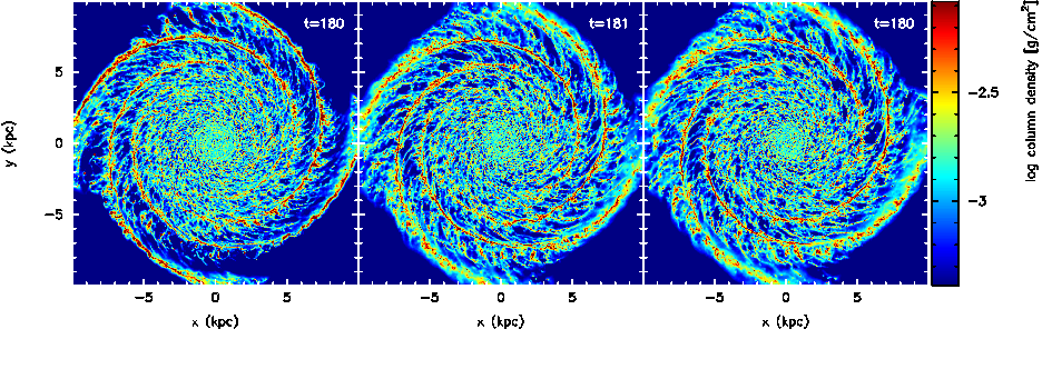
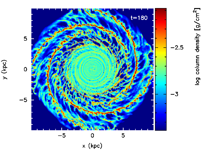
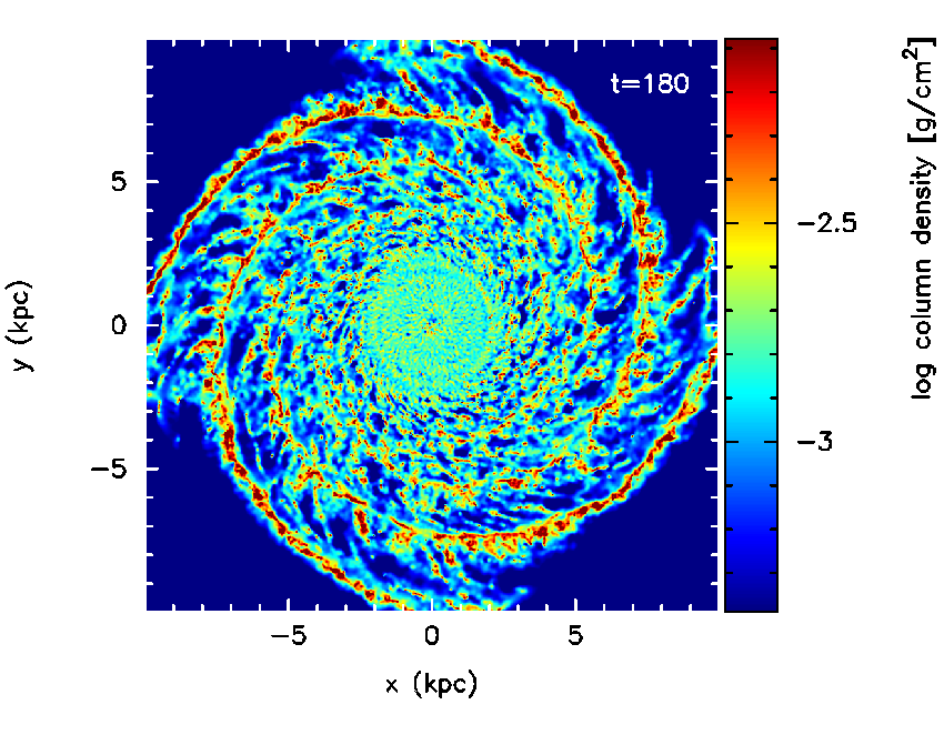
Figure 23: The column density is shown for calculations with a feedback density threshold of 100, 1000 and $10^{4}$ cm^-3 (top row), where a temperature floor of 500 K is imposed (lower left) and with a resolution of 250,000 particles (lower right). The large scale structure is similar in all cases, though the small scale structure is not captured with the imposed temperature floor, or at low resolution. The structure for the case with a threshold of 100 cm^-3 is more similar to Run L1, since the efficiency of star formation is effectively lower.

References

- Bagetakos et al. (2011) Bagetakos I., Brinks E., Walter F., de Blok W. J. G., Usero A., Leroy A. K., Rich J. W., Kennicutt R. C., 2011, AJ, 141, 23
- Bate et al. (1995) Bate M. R., Bonnell I. A., Price N. M., 1995, MNRAS, 277, 362
- Benz et al. (1990) Benz W., Cameron A. G. W., Press W. H., Bowers R. L., 1990, ApJ, 348, 647
- Bigiel et al. (2008) Bigiel F., Leroy A., Walter F., Brinks E., de Blok W. J. G., Madore B., Thornley M. D., 2008, AJ, 136, 2846
- Binney & Tremaine (1987) Binney J., Tremaine S., 1987, Galactic dynamics. Princeton, NJ, Princeton University Press, 1987, 747 p.
- Brunt (2003) Brunt C. M., 2003, ApJ, 583, 280
- Brunt et al. (2009) Brunt C. M., Heyer M. H., Mac Low M., 2009, A&A, 504, 883
- Cepa & Beckman (1990) Cepa J., Beckman J. E., 1990, ApJ, 349, 497
- Chevalier (1974) Chevalier R. A., 1974, ApJ, 188, 501
- Cioffi et al. (1988) Cioffi D. F., McKee C. F., Bertschinger E., 1988, ApJ, 334, 252
- Clarke & Gittins (2006) Clarke C., Gittins D., 2006, MNRAS, 371, 530
- Combes & Becquaert (1997) Combes F., Becquaert J., 1997, A&A, 326, 554
- Cox (2005) Cox D. P., 2005, ARA&A, 43, 337
- Cox & Gómez (2002) Cox D. P., Gómez G. C., 2002, ApJS, 142, 261
- de Avillez (2000) de Avillez M. A., 2000, MNRAS, 315, 479
- de Avillez & Breitschwerdt (2004) de Avillez M. A., Breitschwerdt D., 2004, A&A, 425, 899
- de Avillez & Breitschwerdt (2005) de Avillez M. A., Breitschwerdt D., 2005, A&A, 436, 585
- Dib et al. (2006) Dib S., Bell E., Burkert A., 2006, ApJ, 638, 797
- Dib et al. (2008) Dib S., Brandenburg A., Kim J., Gopinathan M., André P., 2008, ApJL, 678, L105
- Dib & Burkert (2005) Dib S., Burkert A., 2005, ApJ, 630, 238
- Dickey et al. (1990) Dickey J. M., Hanson M. M., Helou G., 1990, ApJ, 352, 522
- Dickey & Lockman (1990) Dickey J. M., Lockman F. J., 1990, ARA&A, 28, 215
- Dobbs (2008) Dobbs C. L., 2008, MNRAS, 391, 844
- Dobbs & Bonnell (2006) Dobbs C. L., Bonnell I. A., 2006, MNRAS, 367, 873
- Dobbs & Bonnell (2007) Dobbs C. L., Bonnell I. A., 2007, MNRAS, 376, 1747
- Dobbs & Bonnell (2008) Dobbs C. L., Bonnell I. A., 2008, MNRAS, 385, 1893
- Dobbs et al. (2006) Dobbs C. L., Bonnell I. A., Pringle J. E., 2006, MNRAS, 371, 1663
- Dobbs et al. (2011) Dobbs C. L., Burkert A., Pringle J. E., 2011, MNRAS, 413, 2935
- Dobbs et al. (2008) Dobbs C. L., Glover S. C. O., Clark P. C., Klessen R. S., 2008, MNRAS, 389, 1097
- Dobbs & Pringle (2009) Dobbs C. L., Pringle J. E., 2009, MNRAS, 396, 1579
- Douglas et al. (2010) Douglas K. A., Acreman D. M., Dobbs C. L., Brunt C. M., 2010, MNRAS, 407, 405
- Elmegreen & Elmegreen (1986) Elmegreen B. G., Elmegreen D. M., 1986, ApJ, 311, 554
- Evans et al. (2009) Evans N. J., Dunham M. M., Jørgensen J. K., Enoch M. L., Merín B., van Dishoeck E. F., Alcalá J. M., Myers P. C., Stapelfeldt K. R., 2009, ApJS, 181, 321
- Ferrière (2001) Ferrière K. M., 2001, Reviews of Modern Physics, 73, 1031
- Field et al. (2011) Field G., Blackman E., Keto E., 2011, ArXiv:1106.3017
- Foyle et al. (2010) Foyle K., Rix H., Walter F., Leroy A. K., 2010, ApJ, 725, 534
- Fujii et al. (2011) Fujii M. S., Baba J., Saitoh T. R., Makino J., Kokubo E., Wada K., 2011, ApJ, 730, 109
- Gao & Solomon (2004) Gao Y., Solomon P. M., 2004, ApJ, 606, 271
- Gazol et al. (2001) Gazol A., Vázquez-Semadeni E., Sánchez-Salcedo F. J., Scalo J., 2001, ApJL, 557, L121
- Genzel et al. (2010) Genzel et al. 2010, MNRAS, 407, 2091
- Gnedin et al. (2009) Gnedin N. Y., Tassis K., Kravtsov A. V., 2009, ApJ, 697, 55
- Heiles & Troland (2003) Heiles C., Troland T. H., 2003, ApJ, 586, 1067
- Heyer et al. (2001) Heyer M. H., Carpenter J. M., Snell R. L., 2001, ApJ, 551, 852
- Hitschfeld et al. (2009) Hitschfeld M., Kramer C., Schuster K. F., Garcia-Burillo S., Stutzki J., 2009, A&A, 495, 795
- Hopkins et al. (2011) Hopkins P. F., Quataert E., Murray N., 2011, ArXiv e-prints
- Ikeuchi et al. (1984) Ikeuchi S., Habe A., Tanaka Y. D., 1984, MNRAS, 207, 909
- Imara et al. (2011) Imara N., Bigiel F., Blitz L., 2011, ApJ, 732, 79
- Imara & Blitz (2011) Imara N., Blitz L., 2011, ApJ, 732, 78
- Joung & Mac Low (2006) Joung M. K. R., Mac Low M.-M., 2006, ApJ, 653, 1266
- Joung et al. (2009) Joung M. R., Mac Low M., Bryan G. L., 2009, ApJ, 704, 137
- Kennicutt (1989) Kennicutt R. C., 1989, ApJ, 344, 685
- Kennicutt (1998) Kennicutt R. C., 1998, ARA&A, 36, 189
- Kennicutt (2008) Kennicutt Jr. R. C., 2008, in J. H. Knapen, T. J. Mahoney, & A. Vazdekis ed., Pathways Through an Eclectic Universe Vol. 390 of Astronomical Society of the Pacific Conference Series, The Schmidt Law: Is it Universal and What Are its Implications?. pp 149–+
- Kim et al. (2008) Kim C., Kim W., Ostriker E. C., 2008, ApJ, 681, 1148
- Kim et al. (2003) Kim W.-T., Ostriker E. C., Stone J. M., 2003, ApJ, 599, 1157
- Korpi et al. (1999) Korpi M. J., Brandenburg A., Shukurov A., Tuominen I., Nordlund Å., 1999, ApJL, 514, L99
- Koyama & Ostriker (2009) Koyama H., Ostriker E. C., 2009, ApJ, 693, 1316
- Krumholz & Dekel (2010) Krumholz M. R., Dekel A., 2010, MNRAS, 406, 112
- La Vigne et al. (2006) La Vigne M. A., Vogel S. N., Ostriker E. C., 2006, ApJ, 650, 818
- Li et al. (2005) Li Y., Mac Low M.-M., Klessen R. S., 2005, ApJ, 626, 823
- Li et al. (2006) Li Y., Mac Low M.-M., Klessen R. S., 2006, ApJ, 639, 879
- Maíz-Apellániz (2001) Maíz-Apellániz J., 2001, AJ, 121, 2737
- McKee & Cowie (1977) McKee C. F., Cowie L. L., 1977, ApJ, 215, 213
- McKee & Ostriker (2007) McKee C. F., Ostriker E. C., 2007, ARA&A, 45, 565
- McKee & Ostriker (1977) McKee C. F., Ostriker J. P., 1977, ApJ, 218, 148
- McMillan & Ciardullo (1996) McMillan R. J., Ciardullo R., 1996, ApJ, 473, 707
- Mihalas & Binney (1981) Mihalas D., Binney J., 1981, Galactic astronomy: Structure and kinematics /2nd edition/
- Ossenkopf & Mac Low (2002) Ossenkopf V., Mac Low M., 2002, A&A, 390, 307
- Padoan et al. (2009) Padoan P., Juvela M., Kritsuk A., Norman M. L., 2009, ApJL, 707, L153
- Papadopoulos & Pelupessy (2010) Papadopoulos P. P., Pelupessy F. I., 2010, ApJ, 717, 1037
- Pelupessy & Papadopoulos (2009) Pelupessy F. I., Papadopoulos P. P., 2009, ApJ, 707, 954
- Petric & Rupen (2007) Petric A. O., Rupen M. P., 2007, AJ, 134, 1952
- Phillips (1999) Phillips J. P., 1999, Astrophysics & Space Science, 134, 241
- Price (2007) Price D. J., 2007, Publications of the Astronomical Society of Australia, 24, 159
- Price & Monaghan (2007) Price D. J., Monaghan J. J., 2007, MNRAS, 374, 1347
- Reed (2000) Reed B. C., 2000, AJ, 120, 314
- Roberts (1969) Roberts W. W., 1969, ApJ, 158, 123
- Robertson & Kravtsov (2008) Robertson B. E., Kravtsov A. V., 2008, ApJ, 680, 1083
- Rosen & Bregman (1995) Rosen A., Bregman J. N., 1995, ApJ, 440, 634
- Rosolowsky et al. (2003) Rosolowsky E., Engargiola G., Plambeck R., Blitz L., 2003, ApJ, 599, 258
- Saitoh et al. (2008) Saitoh T. R., Daisaka H., Kokubo E., Makino J., Okamoto T., Tomisaka K., Wada K., Yoshida N., 2008, PASJ, 60, 667
- Schmidt (1959) Schmidt M., 1959, ApJ, 129, 243
- Sedov (1959) Sedov L. I., 1959, Similarity and Dimensional Methods in Mechanics
- Seigar & James (2002) Seigar M. S., James P. A., 2002, MNRAS, 337, 1113
- Shetty & Ostriker (2006) Shetty R., Ostriker E. C., 2006, ApJ, 647, 997
- Shetty & Ostriker (2008) Shetty R., Ostriker E. C., 2008, ApJ, 684, 978
- Shostak & van der Kruit (1984) Shostak G. S., van der Kruit P. C., 1984, A&A, 132, 20
- Slyz et al. (2005) Slyz A. D., Devriendt J. E. G., Bryan G., Silk J., 2005, MNRAS, 356, 737
- Swinbank et al. (2010) Swinbank et al. 2010, Nature, 464, 733
- Tamburro et al. (2009) Tamburro D., Rix H., Leroy A. K., Mac Low M., Walter F., Kennicutt R. C., Brinks E., de Blok W. J. G., 2009, AJ, 137, 4424
- Tan (2010) Tan J. C., 2010, ApJL, 710, L88
- Tasker (2011) Tasker E. J., 2011, ApJ, 730, 11
- Tasker & Bryan (2008) Tasker E. J., Bryan G. L., 2008, ApJ, 673, 810
- Tasker & Tan (2009) Tasker E. J., Tan J. C., 2009, ApJ, 700, 358
- Urquhart et al. (2011) Urquhart J. S., Moore T. J. T., Hoare M. G., Lumsden S. L., Oudmaijer R. D., Rathborne J. M., Mottram J. C., Davies B., Stead J. J., 2011, MNRAS, 410, 1237
- van der Kruit & Shostak (1982) van der Kruit P. C., Shostak G. S., 1982, A&A, 105, 351
- van Zee & Bryant (1999) van Zee L., Bryant J., 1999, AJ, 118, 2172
- Wada (2008) Wada K., 2008, ApJ, 675, 188
- Wada et al. (2011) Wada K., Baba J., Saitoh T. R., 2011, ApJ, 735, 1
- Wada & Koda (2004) Wada K., Koda J., 2004, MNRAS, 349, 270
- Wada et al. (2000) Wada K., Spaans M., Kim S., 2000, ApJ, 540, 797
- Wilson et al. (2010) Wilson et al. 2010, MNRAS, pp 1674–+
- Wolfire et al. (2003) Wolfire M. G., McKee C. F., Hollenbach D., Tielens A. G. G. M., 2003, ApJ, 587, 278
- Woltjer (1972) Woltjer L., 1972, ARA&A, 10, 129
- Wong & Blitz (2002) Wong T., Blitz L., 2002, ApJ, 569, 157