Morphology change of the silicon surface induced by Ar⁺ ion beam sputtering

Abstract

Two-level modeling for nanoscale pattern formation on silicon target by Ar⁺ ion sputtering is presented. Phase diagram illustrating possible nanosize surface patterns is discussed. Scaling characteristics for the structure wavelength dependence versus incoming ion energy are defined. Growth and roughness exponents in different domains of the phase diagram are obtained. ion-beam sputtering, surface morphology, nanoscale structures 68.55.-a, 68.35.Ct, 79.20.Rf, 81.16.Rf

Abstract

Проводиться теоретичне дослiдження процесiв змiни морфологiї поверхнi кремнiю при розпиленнi його iонами аргону в рамках дворiвневої схеми, що враховує методи Монте-Карло та модифiковану теорiю Бредлi-Харпера. Отримано та проаналiзовано фазову дiаграму у площинi кут падiння налiтаючого iону та енергiя iону, що iлюструє можливi типи поверхневих нано-структур. Отримано узагальнену степеневу залежнiсть довжини хвилi отриманих поверхневих структур вiд енергiї налiтаючих iонiв. Проаналiзовано показник росту i повздовжнiй та поперечний показники шорсткостi отриманих поверхонь. iонне розпилення, морфологiя поверхнi, нано-структури

1 Introduction

It is well known that low and medium energy ion sputtering may induce a fabrication of periodic nanoscale structures on an irradiated surface [1]. Depending on the sputtered substrate characteristics and sputtering conditions, different types of nanoscale structures such as ripples, nanoholes and nanodots can grow on a target during ion beam sputtering [2, 3, 4, 5, 6]. These patterns have been found on both amorphous and crystalline materials including insulators, semiconductors and metals (see reference [7] and citations therein). Main theoretical models describing ripple formation are based on the results of famous works by Bradley and Harper [4], Kardar et al. [8], Wolf and Villian [9], and Kuramoto et al. [10]. The main control parameters in these models reduced to surface tensions, tilt-dependent erosion rates and diffusion constants are determined by sputtered substrate characteristics and sputtering conditions (see for example [7]).

Among theoretical investigations there are a lot of experimental data manifesting a large class of patterns formed due to the self-organization process. It was experimentally shown that the main properties of pattern formation processes depend on ion-beam parameters such as ion flux, energy of deposition, angle of incidence, and temperature of the substrate (target). Therefore, to study the ion beam sputtering processes theoretically one needs to determine the mentioned parameters of the model according to the physical conditions related to concrete materials.

One of the most frequently used materials for ion beam sputtering is silicon because it is the mainstream material in modern microelectronic industry and it is readily available with high purity and quality. Nanostructuring of silicon has received much attention due to its potential application in developing the Si light sources [11]. Various techniques such as acid etching, ion implantation, reactive evaporation, chemical vapor deposition and molecular beam epitaxy have been used in developing the Si nanomaterials (porous Si, Si nanocrystal-doped dielectrics and Si quantum dots) (see reference [11] and citation therein).

In this paper we study the properties of the formation of nanoscale patterns on a silicon target sputtered by Ar⁺ ions. To this end, we use a two-level scheme, based on Monte-Carlo simulations and the modified Bradley-Harper theory. In the first approach we compute the ion energy dependent penetration depth, widths of the ion energy distribution and sputtering yield. Next, we exploit these characteristics as input data for the continuum approach describing the evolution of the surface height field. We define the domains of values for the angle of incidence and ion energy where different nanoscale structures can be formed. The dynamics of nanoscale pattern formation is discussed. We will show that at fixed values for the incidence angle, one has two scaling exponents for wavelength related to small and large values for ion energy. In addition, we obtain roughness and growth exponents.

The work is organized in the following manner. In section 2 we present the theoretical model in the framework of the modified Bradley-Harper approach. In section 3 using Monte-Carlo modeling we compute the main characteristics incorporated into the continuum theory. The related phase diagram, the dynamics of the formation of nanoscale structures, the ion energy dependent wavelength and scaling properties of the surface morphology are discussed in section 4. We conclude in the last section.

2 Theoretical model

Let us consider a $d$-dimensional substrate and denote with $\mathbf{r}$ the $d$-dimensional vector locating a point on it. The surface is described at each time $t$ by the height $z=h(\mathbf{r},t)$. If we assume that the surface morphology changes during ion sputtering, then we can use the model for the surface growth proposed by Bradley and Harper [4] and further developed by Cuerno and Barabasi [2]. We consider the system where the direction of the ion beam lies in $x-z$ plane at an angle $\theta$ to the normal of the uneroded surface. Following the standard approach one assumes that an averaged energy deposited at the surface (let say at point $O$), due to the ion arriving at the point $P$ in the solid, follows the Gaussian distribution [4] $E(\mathbf{r})=\left[\varepsilon/(2\pi)^{3/2}\sigma\mu^{2}\right]\exp\left[-z^{2}/2\sigma^{2}-(x^{2}+y^{2})/2\mu^{2}\right]$; $\varepsilon$ denotes the kinetic energy of the arriving ion, $\sigma$ and $\mu$ are the widths of distribution in directions parallel and perpendicular to the incoming beam. Parameters $\sigma$ and $\mu$ depend on the target material and can vary with physical properties of the target and incident energy. The erosion velocity at the surface point $O$ is described by the formula $v=p\int_{\mathcal{R}}{\rm d}\mathbf{r}\Phi(\mathbf{r})E(\mathbf{r})$, where integration is provided over the range of the energy distribution of all ions; here $\Phi(\mathbf{r})$ are the corrections for the local slope dependence of the uniform flux $J$. The material constant $p$ is defined as: $p=3/(4\pi^{2})(NU_{0}C_{0})^{-1}$, where $U_{0}$ and $C_{0}$ are the surface binding energy and the constant proportional to the square of the effective radius of the interatomic interaction potential, respectively [12]. The general expression for the local flux for surfaces with non-zero local curvature is [13]:

$$\Phi(x,y,h)=J\cos\left[\arctan\left(\sqrt{(\nabla_{x}h)^{2}+(\nabla_{y}h)^{2}}\right)\right].$$

Hence, the dynamics of the surface height is defined by the relation $\partial_{t}h\simeq-v\left(\theta-\nabla_{x}h,\nabla_{x}^{2}h,\nabla_{y}^{2}h\right)$ and is given by the equation $\partial_{t}h\simeq-v(\theta)\sqrt{1+(\nabla h)^{2}}$, where $0<\theta<\pi/2$ [4, 14, 2, 8, 3]. The linear term expansion yields $\partial_{t}h=-v_{0}+\gamma\nabla_{x}h+\nu_{\alpha}\nabla_{\alpha\alpha}^{2}h$; where $\nabla=\partial/\partial\mathbf{r}$, $\nabla_{\alpha}=\partial/\partial\alpha$, $\alpha=\{x,y\}$. Here $v_{0}$ is the surface erosion velocity; $\gamma=\gamma(\theta)$ is a constant that describes the slope depending erosion; $\nu_{\alpha}=\nu_{\alpha}(\theta)$ is the effective surface tension generated by erosion process in $\alpha$ direction.

If one assumes that the surface current is driven by differences in chemical potential $\mu$, then the evolution equation for the field $h$ should take into account the term $-\nabla\cdot\mathbf{j}_{s}$ in the right hand side, where $\mathbf{j}_{s}=K\nabla(\nabla^{2}h)$ is the surface current; $K>0$ is the temperature dependent surface diffusion constant. If the surface diffusion is thermally activated, then we have $K=D_{s}\kappa\rho/n^{2}T$, where $D_{s}=D_{0}\exp\left(-E_{a}/T\right)$ is the surface self-diffusivity ($E_{a}$ is the activation energy for surface diffusion), $\kappa$ is the surface free energy, $\rho$ is the areal density of diffusing atoms, $n$ is the number of atoms per unit volume in the amorphous solid. This term in the dynamical equation for $h$ is relevant in high temperature limit which will be studied below.

Assuming that the surface varies smoothly, we neglect spatial derivatives of the height $h$ of third and higher orders in the slope expansion. Taking into account nonlinear terms in the slope expansion of the surface height dynamics, we arrive at the equation for the quantity $h^{\prime}=h+v_{0}t$ of the form [4, 2]

$$\partial_{t}h=\gamma\nabla_{x}h+\nu_{\alpha}\nabla_{\alpha\alpha}^{2}h+\frac{1}{2}\lambda_{\alpha}(\nabla_{\alpha}h)^{2}-K\nabla^{2}(\nabla^{2}h)+\xi(x,y,t),\qquad\alpha=\{x,y\},$$ (1)

where we drop the prime for convenience. Here we introduce the uncorrelated white Gaussian noise $\xi$ with zero mean mimicking the randomness resulting from the stochastic nature of the ion arrival to the surface. In equation (1) the effective surface tensions $\nu_{x}$ and $\nu_{y}$ generated by the IBS, the tilt-dependent erosion rates $\lambda_{x}$ and $\lambda_{y}$ are defined through the incident angle $\theta$, penetration depth of incident ion $a$, distribution widths $\sigma$, $\mu$ and the sputtering yield $Y_{0}$ as follows [4, 2]:

$$\gamma = F_{0}\frac{s}{f^{2}}\left[a_{\sigma}^{2}a_{\mu}^{2}c^{2}\left(a_{\sigma}^{2}-1\right)-a_{\sigma}^{4}s^{2}\right],$$

$$\nu_{x} = F_{0}a\frac{a_{\sigma}^{2}}{2f^{3}}\left(2a_{\sigma}^{4}s^{4}-a_{\sigma}^{4}a_{\mu}^{2}s^{2}c^{2}+a_{\sigma}^{2}a_{\mu}^{2}s^{2}c^{2}-a_{\mu}^{4}c^{4}\right),$$

$$\nu_{y} = -F_{0}a\frac{c^{2}a_{\sigma}^{2}}{2f}\,,$$

$$\lambda_{x} = F_{0}\frac{c}{2f^{4}}\left\{a_{\sigma}^{8}a_{\mu}^{2}s^{4}\left(3+2c^{2}\right)+4a_{\sigma}^{6}a_{\mu}^{4}c^{4}s^{2}-a_{\sigma}^{4}a_{\mu}^{6}c^{4}\left(1+2s^{2}\right)\right.$$

$${}-\left.f^{2}\left[2a_{\sigma}^{4}s^{2}-a_{\sigma}^{2}a_{\mu}^{2}\left(1+2s^{2}\right)\right]-a_{\sigma}^{8}a_{\mu}^{4}c^{2}s^{2}-f^{4}\right\},$$

$$\lambda_{y} = F_{0}\frac{c}{2f^{2}}\left(a_{\sigma}^{4}s^{2}+a_{\sigma}^{2}a_{\mu}^{2}c^{2}-a_{\sigma}^{4}a_{\mu}^{2}c^{2}-f^{2}\right).$$ (2)

Here we have used the following notations:

$$F_{0}\equiv\frac{J\varepsilon Y_{0}pa}{\sigma\mu\sqrt{2\pi f}}\exp\left(\frac{-a_{\sigma}^{2}a_{\mu}^{2}c^{2}}{2f}\right),$$ (3)

$$a_{\sigma}\equiv\frac{a}{\sigma}\,,\qquad a_{\mu}\equiv\frac{a}{\mu}\,,\qquad s\equiv\sin(\theta),\qquad c\equiv\cos(\theta),\qquad f\equiv a_{\sigma}^{2}s^{2}+a_{\mu}^{2}c^{2}.$$ (4)

Let us perform the stability analysis for a system with additive fluctuations. To this end, we average the Langevin equation (1) over noise and obtain

$${\partial_{t}}\left\langle h\right\rangle=\gamma\nabla_{x}\left\langle h\right\rangle+\nu_{x}\nabla^{2}_{xx}\left\langle h\right\rangle+\nu_{y}\nabla^{2}_{yy}\left\langle h\right\rangle+\frac{\lambda_{x}}{2}\left\langle\left(\nabla_{x}h\right)^{2}\right\rangle+\frac{\lambda_{y}}{2}\left\langle\left(\nabla_{y}h\right)^{2}\right\rangle-K\nabla^{4}\left\langle h\right\rangle.$$ (5)

Considering the stability of the smooth surface characterized by $\langle h\rangle=0$, we can rewrite the linearized evolution equation in the standard form:

$${\partial_{t}}\left\langle h\right\rangle=\left(\hat{\nu}_{\rm ef}+\hat{K}_{\rm ef}\right)\left\langle h\right\rangle,$$ (6)

with notations

$$\hat{\nu}_{\rm ef}=\gamma{\nabla_{x}}+\nu_{x}\nabla_{xx}^{2}+\nu_{y}\nabla_{yy}^{2}\,,\qquad{\hat{K}_{\rm ef}=-K\nabla^{4}}.$$ (7)

It is easy to see that equation (7) admits a solution of the form $\langle h\rangle=A\exp[\ri(k_{x}x+k_{y}y-\omega t)+\chi t]$. Indeed, substituting it into equation (7) and separating real and imaginary parts we get

$$\omega = -\gamma\left(\theta\right)k_{x}\,,$$ (8)

$$\chi = -\nu_{x}\left(\theta\right)k_{x}^{2}-\nu_{y}\left(\theta\right)k_{y}^{2}-K\left(k_{x}^{2}+k_{y}^{2}\right)^{2}.$$ (9)

As far as $F_{0}$ , $f$, $a$ are positive values, hence one has $\nu_{y}<0$, whereas $\nu_{x}$ can change its sign. Therefore, the Bradley-Harper model does not provide for stable smooth surface. Hence, we can conclude that if $\nu_{x}>0$, then ripples (wave patterns) appear in $x$-direction. On the contrary, when $\nu_{x}<0$, equiaxed structures (nanodots/nanoholes) can be formed on an eroded surface. In addition, the sign of the product $\lambda_{x}\cdot\lambda_{y}$ can play a crucial role in ripple formation processes [15].

For the noiseless nonlinear model (1) it was shown that as the sets $\nu_{\alpha}$ and $\lambda_{\alpha}$ are the functions of the angle of incidence $\theta\in[0,\pi/2]$ there are three domains in the phase diagram $(a_{\sigma}\,,\theta)$ where $\nu_{x}$ and $\lambda_{x}$ change their signs, separately [2]. This results in the formation of ripples in different directions $x$ or $y$ varying $a_{\sigma}$ or $\theta$.

One needs to note that in the Bradley-Harper approach describing the processes of ripple formation on amorphous substrates the penetration depth can be approximated as $a(\varepsilon)\sim\varepsilon$ leading to the power-law asymptotics for the wavelength of the ripples $\Lambda$ versus ion energy as follows: $\Lambda\sim\varepsilon^{-1/2}$ [4]. In the next section, performing calculations for the sputtering of the silicon target by Ar⁺ ions we shall show that there are deviations from these asymptotics due to power-law dependence of $a$, $\sigma$, $\mu$ versus ion energy $\varepsilon$. Moreover, it will be shown that the sputtering yield depends on both incident angle $\theta$ end ion energy $\varepsilon$ in a power-law form. To define $a$, $\sigma$, $\mu$ and the sputtering yield, we shall use Monte-Carlo approach.

3 Monte-Carlo modelling

To study the evolution of the silicon surface morphology during Ar⁺ ion beam sputtering one needs to know the energy of ions and target characteristics such as: penetration depth of the Ar⁺ ions into the silicon target $a$; widths of the distribution in parallel and perpendicular directions of the incoming beam ($\sigma$ and $\mu$) and sputtering yield $Y_{0}$ . Moreover, to simulate the target morphology evolution one should define temperature $T$, uniform flux $J$, atomic density of the target $N$, surface binding energy $U_{0}$ and the effective radius of interatomic interaction potential. Using data from reference [5] at $T=550$ C one has $K=C^{\prime}8.49\times 10^{3}$ nm⁴/s, where addimer concentration is $C^{\prime}=0.04$ atoms/site ($\approx 4\%$ coverage), or, $C^{\prime}=0.07$ atoms/nm². To define the material constant $p$ we shall use $N\simeq 50$ atoms/nm³, $U_{0}=4.73$ eV. For the effective radius of interatomic interaction potential, we put the length of the main diagonal of silicon primitive cell with lattice parameter $0.5437$ nm. To compute the time evolution of the silicon surface morphology, we should calculate the effective surface tensions $\nu_{x}$ and $\nu_{y}$ generated by the IBS, and the rates $\lambda_{x}$ and $\lambda_{y}$ [see equation (2)]. Following relations (3) and (4) dependent on ion energy, parameters $a$, $\sigma$ and $\mu$, as far as $Y_{0}=Y_{0}(\theta,\varepsilon)$, can be computed. From experimental point of view, the control parameters at IBS are the energy of ion beam, off-normal incidence angle and ion flux. In all our calculations we put $J=20$ ions/(nm² s). Thereafter we vary the ion energy in the interval $100$ eV$\div 10$ keV and use intermediate off-normal incidence angles $\theta\in[40^{\circ},65^{\circ}]$.

In further study, we use the well-known program codes (TRIM and SRIM) to calculate the stopping range of ions in matter and transport range of ions in matter. Description of algorithms and the basic principles for Monte-Carlo calculation of both the transport range of ions in matter and the stopping range of ions in matter can be found in [16]; TRIM and SRIM codes can be found on the web-site www.srim.org.

Values for parameters $a$, $\sigma$ and $\mu$ for silicon target sputtered by Ar⁺ ions were obtained with the help of SRIM code (a program for calculating the stopping range of ions in matter). Results for relative penetration depths $a_{\sigma}\equiv a/\sigma$ and $a_{\mu}\equiv a/\mu$ versus ion energy are shown in figure 1 (dependencies $a(\varepsilon)$, $\sigma(\varepsilon)$ and $\mu(\varepsilon)$ are shown in the insert).

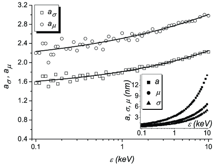
Figure 1: Relative penetration depths of the Ar⁺ ions into the silicon target versus ion energy (penetration depth and distribution widths versus ion energy are shown in insertion).

In figure 1 it is seen that longitudinal and transverse widths $\sigma$ and $\mu$, respectively, as far as $a_{\sigma}$ and $a_{\mu}$ satisfy the following relations, are as follows: $\sigma<\mu$ and $a_{\sigma}<a_{\mu}$ . In reference [17] it was shown that the rotated ripple structures formed when $\lambda_{x}\lambda_{y}<0$ with rotation angle $\varphi=\tan^{-1}\sqrt{-\lambda_{x}/\lambda_{y}}$ can be observed at small incidence angles $\theta$ when $a_{\mu}<a_{\sigma}$ ($a_{\sigma}=1$) and at intermediate and large $\theta$ when $a_{\mu}>a_{\sigma}$ . Hence, one can expect the appearance of rotated ripple structures in our system.

It is principally important that dependencies of penetration depth $a$ and longitudinal and transverse widths $\sigma$ and $\mu$, respectively, versus ion energy $\varepsilon$ deviate from the linear law predicted by Bradley and Harper [4]. For a silicon target sputtered by Ar⁺ ions we have obtained a power-law approximation of the form: $\phi(\varepsilon)=A+B\varepsilon^{C}$, where $\phi=\{a,\sigma,\mu\}$, constants $A$, $B$ and $C$ are fitting parameters. So, we can expect that the wavelength dependence $\Lambda(\varepsilon)\sim\varepsilon^{-\delta}$ can be characterized by the exponent $\delta\neq 1/2$. In our further continuum approach we shall use the obtained power-law asymptotics for $a$, $a_{\sigma}$ and $a_{\mu}$ from Monte-Carlo simulations.

To compute the dependence of the sputtering yield versus ion energy and angle of incidence we use Monte-Carlo approach realized in TRIM code (program for the calculation of transport range of ions in matter). The results of calculations for sputtering yield versus incident angle at fixed ion energy and sputtering yield versus ion energy at fixed incident angle are shown in figures 2 (a) and 2 (b), respectively. In figure 2 it is seen that sputtering yield depends on both ion energy and incidence angle in accordance with a power law as follows $Y_{0}(\psi)=A^{\prime}+B^{\prime}\psi^{C^{\prime}}$, where $\psi=\{\theta,\varepsilon\}$, constants $A^{\prime}$, $B^{\prime}$ and $C^{\prime}$ are fitting parameters. Therefore, all parameters ($\nu_{x}$ , $\nu_{y}$ , $\lambda_{x}$ , $\lambda_{y}$) required to monitor the time evolution of silicon surface morphology during IBS are well defined.

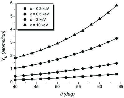
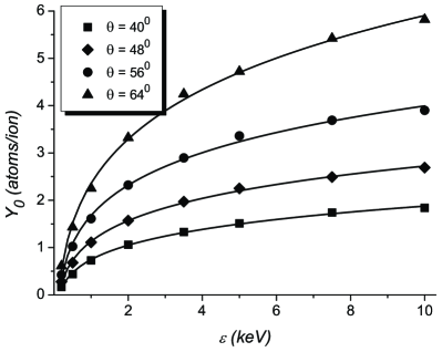
(a)

(b)

Figure 2: Sputtering yield for Ar⁺ in Si at (a) fixed ion energy, (b) fixed incidence angle.

4 Surface morphology change during sputtering

4.1 Phase diagram and typical patterns

Firstly, let us compute a phase diagram $\varepsilon(\theta)$ defining domains for different surface patterns of silicon sputtered by Ar⁺ ions. To this end, we shall monitor a sign change of surface tension $\nu_{x}$ and tilt-dependent erosion rates $\lambda_{x}$ and $\lambda_{y}$ (as it was mentioned above $\nu_{y}$ is always less than 0). The corresponding phase diagram indicating possible patterns is shown in figure 3. We need to stress that in the related interval for both the ion energy and the incidence angle except $\nu_{y}<0$, one has $\lambda_{y}<0$. From figure 3 it follows that plane $(\theta,\varepsilon)$ is divided by three curves into five domains A, B, C, D and E. If one crosses the dash-dot curve, then quantity $\nu_{x}$ changes it sign. Therefore, in the linear regime at small incidence angles $\theta$ (domain A), instability of the silicon surface occurs in both $x$ and $y$ directions due to $\nu_{y}<0$ and $\nu_{x}<0$. In the domain E (at large $\theta$) in the linear regime, patterns are stable in $x$-direction due to $\nu_{x}>0$. At large times (nonlinear regime) the surface morphology is governed by nonlinear parameters $\lambda_{x}$ and $\lambda_{y}$ . Solid curve in figure 3 divides domains characterized by $\lambda_{x}<0$ and $\lambda_{x}>0$. Therefore, between solid and dash-dot lines only $\lambda_{x}$ is positive (domains C and D), whereas in the domain E both $\nu_{x}$ and $\lambda_{x}$ are positive. Dash curve corresponds to the condition $\nu_{x}=\nu_{y}$ . Hence, before the dash curve (domains A and C) when $\nu_{x}<\nu_{y}$, vertical elongated surface structures should be formed, whereas after the dash curve (domains B, D and E), the corresponding structures should be of a horizontal elongated type.

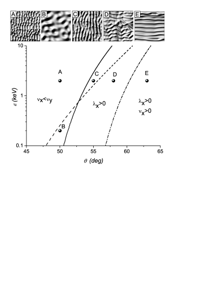
Figure 3: Phase diagram and typical surface patterns.

To illustrate typical structures in each domain in figure 3 we numerically solve equation (1) on quadratic lattice $L\times L$ of the linear size $L=256$ with periodic boundary conditions. Spatial derivatives of the second and fourth orders were computed according to the standard finite-difference scheme; the nonlinear term $(\nabla h)^{2}$ was computed according to the scheme proposed in references [18, 19]. We have used Gaussian initial conditions taking $\langle h({\bf r},t=0)\rangle=0$ and $\langle(\delta h)^{2}\rangle=0.1$; the integration time step is $\Delta t=0.005$ and the space step is $\ell=1$.

Typical surface patterns in domains (A–E) are shown in figure 3. It is seen that on the left hand side of the solid curve when $\nu_{y}<0$ and $\nu_{x}<0$, pattern type of holes is realized (see snapshots A and B). It follows that patterns realized at high energy ions are characterized by small size (see snapshot A), whereas at small $\varepsilon$ one has large-scale patterns (see snapshot B). Moreover, orientation of holes in points A and B is different. It is defined by a minimal value of both $\nu_{x}$ and $\nu_{y}$ . Structures, shown by snapshots C and D (ripples) are characterized by positive value of parameter $\lambda_{x}$ , which defines nonlinear effects in $x$-direction. An orientation of the corresponding ripples is defined by a minimal value of both $\nu_{x}$ and $\nu_{y}$ as in the previous case. Hence, as far as $\nu_{x}<\nu_{y}$ from the left of the dashed curve in figure 3, the related patterns in domains A and C are elongated in $y$ direction. On the contrary, in snapshots B, D, and E there are horizontal elongated structures. Structures in snapshots A, B, C and D are characterized by instabilities in both $x$ and $y$ directions due to $\nu_{x}<0$ and $\nu_{y}<0$. In the domain, indicated by point E due to $\nu_{x}>0$, structures are stable in $x$ direction.

The obtained phase diagram is in good correspondence with the results of experimental studies of the dynamics of the surface Si(001) sputtered by Ar⁺ ions [20], where according to the experimentally obtained a phase diagram in the plane ‘‘ion energy – angle of incidence’’ it was shown that if the angle of incidence or ion energy varies, then orientation of ripples can be changed. It is important that in the considered interval of incidence angle, the obtained phase diagram in figure 3 is topologically similar to the experimental one. However, nonlinear KS equation (1) with parameters defined by equations (2)–(4) does not presume a stable smooth surface because $\nu_{y}$ is a negative quantity.

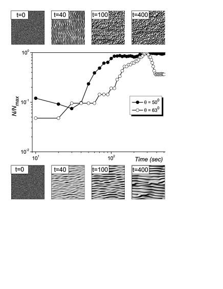
Figure 4: Relative number of islands at $\varepsilon=2$ keV and characteristic snapshots at $\theta=50^{\circ}$ (top) and $\theta=63^{\circ}$ (bottom).

To prove that holes and ripples are stable in time, let us consider the dynamics of the surface morphology change. We analyze two representative kinds of patterns shown in figure 3 as snapshots A and E and compute the number of islands for each pattern in time. To this end, we have cut the surface $h(x,y)$ at an average height level $\langle h\rangle$ and calculated the relative number of islands $N/N_{\rm max}$ at fixed times, where $N_{\rm max}$ is a maximal value of islands. In our computation scheme we used the following definition for the island: all points on the surface with $h<\langle h\rangle$ belonging to one manifold having a closed boundary, form an island. The corresponding boundary of the island was obtained according to the percolation model formalism. Results for relative number of islands were averaged over 20 independent runs. Typical evolution of the number of islands is shown in figure 4 at $\varepsilon=2$ keV for $\theta=50^{\circ}$ and $\theta=63^{\circ}$. It is seen that the relative number of islands grows at small time interval that corresponds to processes of the formation of islands. At intermediate times, the relative number of islands decreases which means a realization of coalescence processes. It is important that in the process of ripple formation the coalescence regime is well pronounced (see empty circles). On the contrary, for the process of nanohole formation (filled circles), this such regime is only weakly observed. At large times one has a stationary behavior of the relative number of islands. Hence, processes of ripple and nanohole formation are stationary ones: at large time intervals the averaged number of islands does not change in time. Snapshots of the silicon surface morphology for $\theta=50^{\circ}$ and $\theta=63^{\circ}$ at $t=0$, $40$, $100$ and $400$ seconds are shown in figure 4 in the top and in the bottom of the figure, respectively.

4.2 Wavelength dependence on the ion energy

Next, let us study the wavelength dependence on the incident ion energy and on the angle of incidence. As it was shown earlier in the Bradley-Harper theory, a relation between parameters $\nu_{x}$ and $\nu_{y}$ determines the orientation of surface patterns. The wavelength of selected patterns in the corresponding direction is defined as follows: $\Lambda_{x,y}=2\pi\sqrt{2K/|\nu_{\min x,y}|}$, where $\nu_{\min x,y}=\min(\nu_{x}\,,\nu_{y})$. One needs to note that following the phase diagram shown in figure 3, a variation in the ion energy at fixed angles of incidence causes a change in the orientation of structures: at small $\varepsilon$ one has structures elongated in $y$ direction, whereas at large $\varepsilon$, structures are horizontally elongated. Corresponding dependencies of the wavelength versus ion energy at fixed values for incidence angle are shown in figure 5.

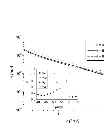
Figure 5: Dependence of the wavelength on the ion energy (the scaling exponent $\delta$ dependence on the incident angle is shown in insertion).

It is seen that the wavelength decreases with the ion energy growth according to a power law and varies in the interval from $100$ nm to $1~{}\mu$m. This result is in good correspondence with experimental data for sputtering of the silicon target by Ar⁺ ions [5]. It is principally important that as far as the penetration depth depends on the ion energy in a nonlinear manner (see the insert in figure 1) one can expect a deviation from the Bradley-Harper wavelength asymptote $\Lambda\sim\varepsilon^{-1/2}$. In figure 5 it is seen that at small and large incidence angles (see dot and dash lines, respectively) one has linear dependencies in log-log plot characterized by the corresponding unique slope. However, at intermediate values for $\theta$ related to the dash curve in figure 3, the dependence $\Lambda(\varepsilon)$ has a kink. This kink means a change in the orientation of patterns. In such a case one has two slopes at small energies, i.e., before kink, one has selected the patterns characterized by $\Lambda_{x}$ , whereas at large energies the patterns are defined by $\Lambda_{y}$ (see solid line and asymptotics in figure 5). Therefore, at small ion energies the patterns are oriented in $y$ direction, whereas at large ion energies they are oriented in $x$ direction. Hence, for the wavelength dependence on the ion energy one can write $\Lambda\sim\varepsilon^{-\delta}$ where the scaling exponent $\delta$ is defined as a slope of the dependence $\Lambda(\varepsilon)$ in double logarithmic plot before and after the kink. The dependence of the scaling exponent versus incidence angle is shown as an insert in figure 5. One can see that for the described interval for the angle of incidence $\delta>1/2$. Moreover, at small and large $\theta$ the exponent $\delta$ does not essentially change it values, whereas in the interval for $\theta$ when $\Lambda(\varepsilon)$ has a kink, the exponent $\delta$ varies from $0.65$ toward $1.05$. We should note that the obtained picture is realized when the incoming ion flux $J$ and temperature $T$ are constants. In the opposite case, variation in $J$ and $T$ leads to the known asymptotes: $\Lambda\propto J^{-1/2}$, $\Lambda\propto T^{-1/2}\exp(-E_{a}/2T)$, where $E_{a}$ is an activation energy.

4.3 Scaling properties of patterns

Finally, let us study the scaling properties of the surface patterns, computing growth and roughness exponents. To this end, we analyze a height-height correlation function $C_{h}(r,t)=\langle[h(r+r^{\prime},t)-h(r^{\prime},t)]^{2}\rangle$. In the framework of dynamic scaling hypothesis following references [21, 22], one arrives at scaling relations $C_{h}(t)\propto t^{2\beta}$, $C_{h}(r)\propto r^{2\alpha}$, allowing one to define the growth exponent $\beta$ and the roughness exponent $\alpha$.

In reference [23] it was shown that there is a set of exponents $\{\beta\}$ describing the universal behavior of the correlation function at early stages of the system evolution. At late times where a true scaling regime is observed there is a unique value for $\beta$. The roughness exponent $\alpha$ takes similar values at different time windows and can be considered as a constant depending on the system parameters only. From practical viewpoint, the analysis of the surface growth is urgent at large time intervals where the true scaling regime is observed and there is no essential difference in values $\beta$ at different time windows. It is known that anisotropic surfaces studied in this paper may exhibit a more complex dynamic scaling behaviour than isotropic ones because anisotropy of the surface is reflected in lateral correlations of the surface roughness [24, 25]. In reference [6] it was proposed to use local roughness scales $\alpha_{x}$ , $\alpha_{y}$ in the directions normal and parallel to the projection direction of the ion beam. Values for growth and roughness exponents together with surface tensions $\nu_{x}$ and $\nu_{y}$ at $\varepsilon=2$ keV and fixed values for incidence angle are presented in table 1. It is seen that when $\nu_{x}<\nu_{y}$, a relation $\alpha_{x}>\alpha_{y}$ is realized due to orientation of the structures in $y$ direction. On the contrary, if $\nu_{x}>\nu_{y}$ holds, then one has $\alpha_{x}<\alpha_{y}$ . Hence, making an analysis of the obtained scaling exponents, one can conclude that if structures are oriented in $y$ direction, then roughness is larger in $x$-direction and vice versa (compare patterns in snapshots A, C, D and E in figure 3 with exponents in table 1). The obtained results for growth and roughness exponents are in good correspondence with experimental studies of the silicon target sputtered by Ar⁺ ions (see [6, 26]).

Table 1: Growth and roughness scaling exponents at $\varepsilon=2$ keV.

	$\theta$	$\alpha_{x}$	$\alpha_{y}$	$\beta$	$\nu_{x}$	$\nu_{y}$
	$50^{\circ}$	0.90	0.82	0.23	–0.222	–0.151
	$55^{\circ}$	0.94	0.90	0.22	–0.137	–0.127
	$58^{\circ}$	0.90	0.95	0.21	–0.067	–0.112
	$63^{\circ}$	0.89	0.99	0.17	0.086	–0.087

5 Conclusions

Two-level modeling for nanoscale pattern formation on silicon target induced by Ar⁺ ion sputtering has been reported. We have used Monte-Carlo simulations and a continuum approach based on the Bradley-Harper theory. It was shown that for the described system, the dependencies of the averaged penetration depth of the incident ion and the corresponding distribution widths of the deposited energy in directions parallel and perpendicular to the incoming beam versus ion energy are of the power-law form. Varying the incoming ion energy and ion incidence angle, we have defined the sputtering yield with the help of Monte-Carlo simulations. The obtained results have been used in the modified Bradley-Harper theory within the framework of two-scale modeling scheme.

We have computed a phase diagram for control parameters: i.e., incidence angle and ion energy that defines possible patterns on silicon target sputtered by Ar⁺ ions. It was shown that at small incidence angles, nanohole patterns are realized, whereas at large incidence angles, pattern type of ripples is observed. Analyzing the morphology change of silicon surface we have shown that during the system evolution, the number of nanoholes/ripples becomes constant, indicating stability of the obtained structures in time.

We have found that there are deviations from the Bradley-Harper asymptotics for the wavelength dependence on the ion energy. Moreover, when the orientation of patterns changes, a kink is realized in such asymptotics. The exponent of such power-law asymptotics depends on the angle of incidence. At fixed values for incidence angle one has two scaling exponents related to small and large values for the ion energy according to a change in the orientation of structures. While studying the scaling characteristics of the height-height correlation function, the growth exponent together with longitudinal and transverse roughness exponents are obtained for different values of incidence angle at a fixed ion energy. It was shown that relations between roughness exponents are defined through relations between corresponding effective surface tensions.

The results obtained in a two-scale modeling scheme are in good correspondence with the known theoretical and experimental data for sputtering of silicon target by Ar⁺ ions in the considered interval of values for incidence angle of ions, the incoming ion energy, temperature and ion flux [5, 20, 6, 27, 26].

Змiна морфологiї поверхнi кремнiю при розпиленнi його iонами аргонуВ.О. Харченко, Д.О. Харченко Iнститут прикладної фiзики НАН України, вул. Петропавлiвська 58, 40030 Суми, Україна

References

-
[1]
Frost F., Ziberty B., Schindler A., Rauschenbach B., Appl.
Phys. A, 2008, 91, 551;
doi:10.1007/s00339-008-4516-0. - [2] Cuerno R., Barabasi A.-L., Phys. Rev. Lett., 1995, 74, 4746; doi:10.1103/PhysRevLett.74.4746.
- [3] Makeev M., Barabasi A.-L., Appl. Phys. Lett., 1997, 71, 2800; doi:10.1063/1.120140.
- [4] Bradley R.M., Harper J.M.E., J. Vac. Sci. Technol. A, 1988, 6, 2390; doi:10.1116/1.575561.
-
[5]
Erlebacher J., Aziz M.J., Chason E., Sinclair M.B., Floro J.A., J. Vac. Sci. Technol. A, 2000, 18, 115;
doi:10.1116/1.582127. -
[6]
Keller A., Cuerno R., Facsko S., Moller W., Phys. Rev. B,
2009, 79, 115437;
doi:10.1103/PhysRevB.79.115437. - [7] Makeev M., Cuerno R., Barabasi A.-L., Nucl. Instrum. Meth. B, 2002, 197, 185; doi:10.1016/S0168-583X(02)01436-2.
- [8] Kardar M., Parisi G., Zhang Y.-C., Phys. Rev. Lett., 1986, 56, 889; doi:10.1103/PhysRevLett.56.889.
- [9] Wolf D.E., Villian J., Europhys. Lett., 1990, 13, 389; doi:10.1209/0295-5075/13/5/002.
- [10] Kuramoto Y., Tsuzuki T., Prog. Theor. Phys., 1976, 55, 356; doi:10.1143/PTP.55.356.
- [11] Bisi O., Campisano S.U., Pavesi L., Priolo F. (Eds.), Silicon Based Microphotonics: From Basic to Applications. IOS Press, Amsterdam, 1999.
- [12] Sigmund P., J. Mater. Sci., 1973, 8, 1545; doi:10.1007/BF00754888.
-
[13]
Makeev M.A., Barabasi A.-L., Nucl. Instrum. Meth. B, 2004,
222, 316;
doi:10.1016/j.nimb.2004.02.027. - [14] Cahn J.W., Taylor J.E., Acta Mater., 1994, 42, 1045; doi:10.1016/0956-7151(94)90123-6.
- [15] Rost M., Krug J., Phys. Rev. Let., 1995, 75, 3894; doi:10.1103/PhysRevLett.75.3894.
- [16] Ziegler J.F., Biersack J.P. and Littmark U., The Stopping and Range of Ions in Solids. Vol.1, Pergamon Press, 1985.
- [17] Kahng B., Kim J., Curr. Appl. Phys., 2004, 4, 115; doi:10.1016/j.cap.2003.10.010.
- [18] Lam C.H., Shin F.G., Phys. Rev. E, 1998, 57, 6506; doi:10.1103/PhysRevE.57.6506.
- [19] Giada L., Giacometti A., Rossi M., Phys. Rev. E, 2002, 65, 036134; doi:10.1103/PhysRevE.66.019902.
- [20] Madi C.S., Davidovitch B., George H.B., Norris S.A., Brenner M.P., Aziz M.J., Phys. Rev. Lett., 2008, 101, 246102; doi:10.1103/PhysRevLett.101.246102.
-
[21]
Sinha S.K., Sirota E.B., Garott S., Stanley H.B.,
Phys. Rev. B, 1988, 38, 2297;
doi:10.1103/PhysRevB.38.2297. - [22] Giada L., Giacometti A., Rossi M., Phys. Rev. E, 2002, 65, 036134; doi:10.1103/PhysRevE.65.036134.
-
[23]
Kharchenko D.O., Kharchenko V.O., Lysenko I.O., Kokhan S.V.,
Phys. Rev. E, 2010, 82, 061108;
doi:10.1103/PhysRevE.82.061108. -
[24]
Schmittmann B., Pruessner G., Jansses H.-K.,
Phys. Rev. E, 2006, 73, 051603;
doi:10.1103/PhysRevE.73.051603. -
[25]
Pastor-Satorras R., Rothman D.H.,
J. Stat. Phys., 1998, 93, 477;
doi:10.1023/B:JOSS.0000033160.59155.c6. - [26] Chan A.C.-T., Wang G.-C., Surf. Sci., 1998, 414, 14; doi:10.1016/S0039-6028(98)00425-7.
- [27] Erlebacher J., Aziz M.J., Chason E., Sinclair M.B., Floro J.A., Phys. Rev. Lett., 1999, 82, 2330; doi:10.1103/PhysRevLett.82.2330.