Various correlations in a Heisenberg $XXZ$ spin chain both in thermal equilibrium and under the intrinsic decoherence

Abstract

In this paper we discuss various correlations measured by the concurrence (C), classical correlation (CC), quantum discord (QD), and geometric measure of discord (GMD) in a two-qubit Heisenberg $XXZ$ spin chain in the presence of external magnetic field and Dzyaloshinskii-Moriya (DM) anisotropic antisymmetric interaction. Based on the analytically derived expressions for the correlations for the cases of thermal equilibrium and the inclusion of intrinsic decoherence, we discuss and compare the effects of various system parameters on the correlations in different cases. The results show that the anisotropy $J_{z}$ is considerably crucial for the correlations in thermal equilibrium at zero temperature limit but ineffective under the consideration of the intrinsic decoherence, and these quantities decrease as temperature $T$ rises on the whole. Besides, $J$ turned out to be constructive, but $B$ be detrimental in the manipulation and control of various quantities both in thermal equilibrium and under the intrinsic decoherence which can be avoided by tuning other system parameters, while $D$ is constructive in thermal equilibrium, but destructive in the case of intrinsic decoherence in general. In addition, for the initial state $|\Psi_{1}(0)\rangle=\frac{1}{\sqrt{2}}(|01\rangle+|10\rangle)$, all the correlations except the CC, exhibit a damping oscillation to a stable value larger than zero following the time, while for the initial state $|\Psi_{2}(0)\rangle=\frac{1}{\sqrt{2}}(|00\rangle+|11\rangle)$, all the correlations monotonously decrease, but CC still remains maximum. Moreover, there is not a definite ordering of these quantities in thermal equilibrium, whereas there is a descending order of the CC, C, GMD and QD under the intrinsic decoherence with a nonnull $B$ when the initial state is $|\Psi_{2}(0)\rangle$.

I introduction

The most fascinating nonlocal correlation feature of quantum mechanics is the quantum entanglement, generally considered as an essential resource for the quantum information processing NielsenBook that provides the possibility of quantum teleportation BennettPRL1 , quantum dense coding BennettPRL2 , and quantum cryptographic key distribution EkertPRL , etc. Ever since the foundation of the quantum information science, the quantification of the entangled states has been one of the most fundamental and substantial tasks. As is well known, quantum states have been subdivided into entangled states and separable (nonentangled) states. However, recent research reveals that entanglement doesn’t provide all aspects of quantum correlations which arise from the noncommutativity of operators representing states, observables, and measurements LuoPRA1 . Quantum states display other nonlocal correlations not present in the classical counterpart, such as the so-called quantum discord (QD) that is intimately relevant to local measurement which accounts for all nonclassical correlations originally introduced by Ollivier and Zurek OllivierPRL . QD is defined by the distinction between the two quantum extensions of the classical mutual information defined equivalently in two classical ways and shown to be nonzero both theoretically LuoPRA1 ; OllivierPRL and experimentally LanyonPRL for some separable states which may be utilized to speed up some tasks over their classical counterparts. In addition, QD is responsible for the quantum computational efficiency of deterministic quantum computation with one pure qubit in Ref. DattaPRL ; LanyonPRL albeit in the absence of entanglement. Therefore, it is imperative and desirable to study QD aiming at understanding well the relationship between QD and other correlation indicators and also that among the total correlations, genuinely classical correlations and purely quantum ones.

Recently, the QD has been intensively investigated in the literature both theoretically LuoPRA2 ; SarandyPRA ; WerlangPRA1 ; AliPRA ; WerlangPRA2 ; FanchiniPRA ; SunzhaoyuPRA ; LuoPRA3 ; CilibertiPRA ; LiuPRA ; LizhenniPRA ; LiboPRA ; QasimiPRA ; ParasharPRA ; GirolamiPRA ; DillenschneiderPRB ; ShabaniPRL ; LangPRL ; DakicPRL ; StreltsovPRL ; YuanJPB ; SunzheJPB ; GuojinliangJPB ; LuQIC and experimentally LanyonPRL ; XuJinshiNatCommun . Generally, it is somewhat difficult to calculate QD and the analytical solutions can hardly be obtained except for some particular cases, such as the so-called $X$ states AliPRA . Some researches show that QD, concurrence (C) and classical correlation (CC) are respectively independent measures of correlations with no simple relative ordering and QD is more practical than entanglement LanyonPRL . Quite rencently, Dakić $et$ $al$ DakicPRL have introduced an easily analytically computable quantity, geometric measure of discord (GMD), and given a necessary and sufficient condition for the existence of nonzero QD for any dimensional bipartite states. Moreover, the dynamical behavior of QD in terms of decoherence MazieroPRA1 ; MazieroPRA2 ; MazzolaPRL ; YuanJPB ; LuQIC in both Markovian WerlangPRA1 and Non-Markovian FanchiniPRA ; WangPRA ; VasilePRA cases is also taken into account.

In previous studies, the influence of intrinsic (phase) decoherence, a virtually unavoidable effect caused by the interaction of the system with the surrounding environment, on the dynamics of various correlations (C, QD, GMD and CC) using a Heisenberg spin chain as a quantum channel has not been considered. Also the effect of Dzyaloshinskii-Moriya (DM) interaction, which is introduced via the extension of the Anderson superexchange interaction theory by including the spin-orbit coupling effect, on these correlations and the comparison of these quantities have been rarely reported in the literature. On the other hand, due to the good integrability and scalability, the solid state systems NielsenPRA ; WangxiaoguangPRA ; KamtaPRL ; O'ConnorPRA ; SunPRA ; YeoPRA ; AhmadJPB ; CaiOpt have gained great attention. Particularly, the Heisenberg spin chains, as the natural candidates for the realization of the entanglement showed some substantial advantages compared with the other physical systems LossPRA ; LossPRB ; KaneNature ; SorensenNature ; LiuwumingPRL . In addition, by suitable coding, the Heisenberg interaction alone can be used for quantum computation LidarPRL ; DivincenzoNature ; SantosPRA . To this end, in this paper we investigate in detail both the thermal equilibrium and dynamical behaviors of various correlations in a Heisenberg $XXZ$ spin-$\frac{1}{2}$ chain. We find that the anisotropy $J_{z}$ is considerably crucial for these quantities in thermal equilibrium at zero temperature limit but ineffective under the consideration of the intrinsic decoherence, and these quantities decrease as temperature $T$ rises on the whole. Besides, $J$ and $D$ contribute equivalently to these quantities and turn out to be the most efficient controlling parameters. $J$ plays a constructive role and $B$ a detrimental role in the manipulation and control of these quantities both in thermal equilibrium and under the consideration of intrinsic decoherence, while $D$ is constructive in thermal equilibrium, but becomes to be destructive in the decoherent time evolution process in general. Albeit $B$ is detrimental for these quantities, it remains worthy of being studied since the inclusion of it is in practical need such as the nuclear magnetic resonance quantum computing and the superconducting quantum computing. Furthermore, when the initial state is $|\Psi_{1}(0)\rangle=\frac{1}{\sqrt{2}}(|01\rangle+|10\rangle)$, all the correlations except the CC, exhibit a damping oscillation to a stable value larger than zero following the time, while for the initial state $|\Psi_{2}(0)\rangle=\frac{1}{\sqrt{2}}(|00\rangle+|11\rangle)$, all the correlations monotonously decrease, but CC still remains maximum. Moreover, there is not a definite ordering of these quantities in thermal equilibrium, whereas there is a descending order of the CC, C, GMD and QD under the intrinsic decoherence with a non-zero $B$ when the initial state is $|\Psi_{2}(0)\rangle$.

This paper is organized as follows. In section II, we present a brief overview of various correlation measured quantities. Next we study the thermal correlations in a two-qubit Heisenberg $XXZ$ spin chain with DM interaction in the presence of an external magnetic field along the $z$-axis in section III. Subsequently, we turn to the influence of intrinsic decoherence on various quantities in section IV. Finally we conclude the paper in section V.

II Correlation measures for bipartite system

Firstly we give a brief overview of various correlation measures. Given a bipartite quantum state $\rho_{AB}$ in a composite Hilbert space $\mathcal{H}=\mathcal{H}_{A}\otimes\mathcal{H}_{B}$, the concurrence WoottersPRL as an indicator for entanglement between the two qubits is

$$C(\rho_{AB})=\max\{\lambda_{1}-\lambda_{2}-\lambda_{3}-\lambda_{4},0\},$$ (1)

where $\lambda_{i}(i=1,2,3,4)$ are the square roots of the eigenvalues of the ”spin-flipped” density operator $R=\rho\widetilde{\rho}=\rho(\sigma^{y}_{1}\otimes\sigma^{y}_{2})\rho^{*}(\sigma^{y}_{1}\otimes\sigma^{y}_{2})$ in descending order. $\sigma^{y}$ is the Pauli matrix and $\rho^{*}$ denotes the complex conjugation of the matrix $\rho$ in the standard basis $\{|00\rangle,|01\rangle,|10\rangle,|11\rangle\}.$ For the density matrix in the $X$ form, an alternative equivalent expression is given by

$$C(\rho_{AB})=\max\{C_{1},C_{2},0\},$$ (2)

where $C_{1}=2(|\rho_{41}|-\sqrt{\rho_{33}\rho_{22}})$ and $C_{2}=2(|\rho_{32}|-\sqrt{\rho_{44}\rho_{11}}).$

In classical information theory CoverBook , the total amount of correlations between two systems A and B can be represented by the classical mutual information $I(A;B)=H(A)+H(B)-H(A,B),$ where $H(A)\big{(}H(B),H(A,B)\big{)}$ is the Shannon entropy $H=-\sum_{i}p_{i}\log_{2}p_{i},$ $p_{i}$ representing the probability of an event $i$ associated with A (B, AB). By virtue of the Bayes rule, the mutual information can be rewritten as $J(A;B)=H(A)-H(A|B),$ in which $H(A|B)=H(A,B)-H(B)$ is the classical conditional entropy employed to quantify the ignorance of the state of A when one knows the state of B. Despite the equivalency of the two expressions in the classical case, the quantum versions of the two are not equivalent anymore. In the generalized quantum version, the classical probability distributions are replaced by the density operator $\rho$ and the Shannon entropy by the von Neumann entropy WehrlRevModPhys $S(\rho)$=$-\textrm{Tr}$($\rho$$\log_{2}\rho$). Accordingly, the quantum version of the two mutual information expressions can be obtained as

$$\mathcal{I}(\rho_{A};\rho_{B})=S(\rho_{A})+S(\rho_{B})-S(\rho_{AB}),$$ (3)

where $\rho_{A(B)}=\textrm{Tr}_{B(A)}(\rho_{AB})$ is the reduced density matrix of the subsystem A(B) by tracing out the subsystem B(A). The quantum generalization of the conditional entropy is not the simply replacement of Shannon entropy with von Neumann entropy, but through the process of projective measurement on the subsystem B by a set of complete projectors ${B_{k}},$ with the outcomes labeled by $k,$ then the conditional density matrix $\rho_{k}$ becomes

$$\rho_{k}=\frac{1}{p_{k}}(\mathbbm{l}_{A}\otimes{B_{k}})\rho(\mathbbm{l}_{A}\otimes{B_{k}}),$$ (4)

which is the locally post-measurement state of the subsystem B after obtaining the outcome $k$ on the subsystem A with the probability

$$p_{k}=\textrm{Tr}[(\mathbbm{l}_{A}\otimes{B_{k}})\rho(\mathbbm{l}_{A}\otimes{B_{k}})],$$ (5)

where $\mathbbm{l}_{A}$ is the identity operator on the subsystem A. The projectors ${B_{k}}$ can be parameterized as ${B_{k}}=V|k\rangle\langle k|V^{\dagger},k=0,1$ and the transform matrix $V\in U(2)$ SarandyPRA is

$$V=\left(\begin{array}[]{cccc}\cos\theta&e^{-i\phi}\sin\theta\\ e^{i\phi}\sin\theta&-\cos\theta\\ \end{array}\right).$$ (6)

Then the conditional von Neumann entropy (quantum conditional entropy) and quantum extension of the mutual information can be defined as OllivierPRL

$$S(\rho|\{B_{k}\})=\sum_{k}p_{k}S(\rho_{k}),$$ (7)

$$\mathcal{J}(\rho_{AB}|\{B_{k}\})=S(\rho_{A})-S(\rho|\{B_{k}\}).$$ (8)

Following the definition of the CC in Ref.OllivierPRL

$$\mathcal{CC}(\rho_{AB})=\sup_{\{B_{k}\}}\mathcal{J}(\rho_{AB}|\{B_{k}\}),$$ (9)

then QD defined by the difference between the quantum mutual information $\mathcal{I}(\rho_{AB})$ and the $\mathcal{CC}(\rho_{AB})$ is given by

$$\mathcal{QD}(\rho_{AB})=\mathcal{I}(\rho_{AB})-\mathcal{CC}(\rho_{AB}).$$ (10)

If we denote $S_{\min}(\rho_{AB})=\min_{\{B_{k}\}}S(\rho_{AB}|\{B_{k}\}),$ then a variant expression of QD reads SunzhaoyuPRA

$$\mathcal{QD}(\rho_{AB})=S(\rho_{B})-S(\rho_{AB})+S_{\min}(\rho_{AB}).$$ (11)

It is usually difficult to get the analytical expression of QD except for some special cases, thus another correlation measure, GMD, is introduced by Dakić $et$ $al$ DakicPRL to simplify the computation. It is defined as

$$\mathcal{D}_{G}(\rho_{AB})=\min_{\chi}\|\rho-\chi\|^{2},$$ (12)

where the minimum is over the set of zero-discord states and the geometric quantity

$$\|\rho-\chi\|^{2}:=\textrm{Tr}(\rho-\chi)^{2}$$

is the square of Hilbert-Schmidt norm of Hermitian operators. For any two-qubit state in the so-called Bloch basis

$$\hskip 14.22636pt\rho=\frac{1}{4}\sum_{i,j=0}^{3}R_{ij}\sigma_{i}\otimes\sigma_{j}=\frac{1}{4}\bigg{(}\mathbbm{l}_{A}\otimes\mathbbm{l}_{B}+\sum_{i=1}^{3}(x_{i}\sigma_{i}\otimes\mathbbm{l}_{B}\qquad$$

$$\qquad\qquad+y_{i}\mathbbm{l}_{B}\otimes\sigma_{i})+\sum_{i,j=1}^{3}t_{ij}\sigma_{i}\otimes\sigma_{j}\bigg{)},$$ (13)

where $R_{ij}=\textrm{Tr}[\rho(\sigma_{i}\otimes\sigma_{j})],$ $\sigma_{0}=\mathbbm{l}_{2\times 2},$ $\sigma_{i}(i=1,2,3)$ are the Pauli matrices, $\vec{x}=\{x_{i}\}$, $\vec{y}=\{y_{i}\}$ are the three-dimensional Bloch vectors associated with subsystems A, B, and $t_{ij}$ denote the elements in the correlation matrix $T$. Then, a variant expression of GMD is given by

$$\mathcal{D}_{G}(\rho_{AB})=\frac{1}{4}(\|\vec{y}\vec{y}^{\textrm{T}}\|+\|T\|^{2}-k_{\max}),$$ (14)

where $k_{\max}$ is the largest eigenvalue of the matrix $\vec{y}\vec{y}^{\textrm{T}}+T^{\textrm{T}}T$ (in the case of measurement on the subsystem A, one needs to replace $\vec{y}$ with $\vec{x}$ and $T^{\textrm{T}}T$ with $TT^{\textrm{T}}$). An alternative formulation for GMD has been provided in LuoPRA3 . Note that its maximum value is $\frac{1}{2}$ for two-qubit states, so it is appropriate to consider 2$D_{G}$ as a measure of GMD hereafter in order to compare with other correlation measures GirolamiPRA .

III The correlations in a Heisenberg $XXZ$ spin chain in thermal equilibrium

The physical system we discuss here is a two-qubit Heisenberg $XXZ$ spin chain with the DM anisotropic antisymmetric interaction DzyaloshinskiiJPhysChemSolids ; MoriyaPRL under the external magnetic field and its Hamiltonian is written as

$$\hskip 25.60747ptH=\frac{1}{2}[J\left(\sigma_{1}^{x}\sigma^{x}_{2}+\sigma_{1}^{y}\sigma^{y}_{2}\right)+J_{z}\sigma_{1}^{z}\sigma_{2}^{z}+B\left(\sigma_{1}^{z}+\sigma_{2}^{z}\right)\qquad$$

$$\qquad\qquad+D\left(\sigma_{1}^{x}\sigma_{2}^{y}-\sigma_{1}^{y}\sigma_{2}^{x}\right)],$$ (15)

where $J$ and $J_{z}$ are the real coupling constants, $\sigma_{i}^{j}(i=1,2;j=x,y,z)$ are the Pauli matrices. $B$ and $D$ are respectively the $z$-component of the external magnetic field and DM interaction. We are working in units, so that all parameters are dimensionless. The state of a typical solid-state system at thermal equilibrium in temperature $T$ (canonical ensemble) is $\rho(T)=e^{-\frac{H}{kT}}/Z,$ with $Z=\textrm{Tr}(e^{-\frac{H}{kT}})$ the partition function and $k$ the Boltzmann constant. Usually we work with natural unit system $\hbar=k=1$ for simplicity and henceforth.

In the first instance, we derive the analytical expressions for various correlation measured quantities. After some straightforward algebra, one can readily obtain the thermal concurrence

$$C(\rho_{AB})=\max\{\frac{1}{Z}\big{(}2e^{\frac{J_{z}}{2T}}\sinh\frac{\mu}{T}-e^{-\frac{J_{z}}{2T}}\big{)},0\},$$ (16)

where $\mu=\sqrt{J^{2}+D^{2}}$ and $Z=e^{-\frac{2B+J_{z}}{2T}}\big{(}1+e^{\frac{2B}{T}}+2e^{\frac{B+J_{z}}{T}}\cosh\frac{\mu}{T}\big{)}$. Next, in order to gain the thermal CC and thermal QD, one needs to calculate the quantum conditional entropy and minimize it over all possible projective measurements which is the most difficult part. As per Eqs. (4)-(7), after the minimization of the quantum conditional entropy (i.e., to set the derivative of the quantum conditional entropy $S(\rho|\{B_{k}\})$ with respect to angels $\theta$ and $\phi$ to be zero), one can find that the quantum conditional entropy is independent of angle $\phi$, and reaches its minimum value when $\theta=\frac{(2m+1)\pi}{4}$ (m $\in\mathbb{Z}$) for $-J<J_{z}<J$ in the absence of $B$ and $D$. It is independent of $\theta$ when $J_{z}=\pm J$ (i.e., the $XXX$ model, this can be explained from the physical respective as the system is isotropic). Otherwise its minimum value is reached as $\theta=\frac{m\pi}{2}$ (m $\in\mathbb{Z}$). As $B$ and $D$ are introduced, the range of $J_{z}$ ($-J<J_{z}<J)$, in which the quantum conditional entropy reaches its minimum value when $\theta=\frac{(2m+1)\pi}{4}$ (m $\in\mathbb{Z}$), are broadened. Moreover, the effect of $B$ on the dependence of the minimum quantum conditional entropy with respect to angel $\theta$ is different for the antiferromagnetic (AFM) case ($J>0$) and ferromagetic (FM) case ($J<0$) with $D$ fixed. The effect for the AFM case is more significant compared with the case of FM, in which the range of $J_{z}$ ($-J<J_{z}<J)$ widens slightly. While the effect of $D$ on the dependence mentioned above are the same for both the AFM and FM cases when $B$ is fixed. In addition, the range reduces with the rise of the temperature. Thereby, the CC and QD are obtained respectively as

$$\mathcal{CC}(\rho_{AB})=S(\rho_{A})-\min\{\Lambda_{1},\Lambda_{2}\},$$ (17)

$$\mathcal{QD}(\rho_{AB})=S(\rho_{B})-S(\rho_{AB})+\min\{\Lambda_{1},\Lambda_{2}\},$$ (18)

where

$$S(\rho_{A})=S(\rho_{B})=-\lambda_{-}\log_{2}{\lambda_{-}}-\lambda_{+}\log_{2}{\lambda_{+}},$$

$$\lambda_{\pm}=\frac{1}{Z}(e^{-\frac{J_{z}\pm 2B}{2T}}+e^{\frac{J_{z}}{2T}}\cosh\frac{\mu}{T}),$$

$$S(\rho_{AB})=-\sum_{\eta_{i}=1}^{4}\eta_{i}\log_{2}{\eta_{i}},$$

$$\eta_{1,2}=\frac{1}{Z}e^{-\frac{J_{z}\pm 2B}{2T}},\eta_{3,4}=\frac{1}{Z}e^{\frac{J_{z}\pm 2\mu}{2T}},$$

$$\Lambda_{1}=\frac{1}{\ln 4}[\ln 4-(1-\delta)\ln(1-\delta)-(1+\delta)\ln(1+\delta)],$$

$$\delta=\frac{2\sqrt{(e^{\frac{2B}{T}}-1)^{2}+4e^{\frac{2(B+J_{z})}{T}}\sinh^{2}\frac{\mu}{T}}}{1+e^{\frac{2B}{T}}+2e^{\frac{B+J_{z}}{T}}\cosh\frac{\mu}{T}},$$

and

$$\Lambda_{2}=(\eta_{1}+\omega)(\xi_{-}+\xi_{+})+(\eta_{2}+\omega)(\zeta_{-}+\zeta_{+}),$$

$$\xi_{\pm}=-\frac{1\pm\nu_{1}}{\ln 4}\ln(\frac{1\pm\nu_{1}}{2}),\zeta_{\pm}=-\frac{1\pm\nu_{2}}{\ln 4}\ln(\frac{1\pm\nu_{2}}{2}),$$

$$\omega=\frac{1}{Z}e^{\frac{J_{z}}{2T}}\cosh\frac{\mu}{T},\nu_{1,2}=\frac{\sqrt{(e^{\frac{J_{z}+B}{T}}\cosh\frac{\mu}{T}-1)^{2}}}{1+e^{\frac{J_{z}\pm B}{T}}\cosh\frac{\mu}{T}}.$$

Finally, according to Eqs. (II) and (14), thermal GMD can be written as

$$2\mathcal{D}_{G}(\rho_{AB})=\Omega-\frac{1}{2}\max\{\Gamma_{1},\Gamma_{2}\},$$ (19)

in which

$$\Omega=\frac{2e^{-\frac{J_{z}}{T}}\cosh\frac{2B}{T}-4\cosh\frac{B}{T}\cosh\frac{\mu}{T}+e^{\frac{J_{z}}{T}}(3\cosh\frac{2\mu}{T}-1)}{Z^{2}},$$

$$\Gamma_{1}=\frac{4e^{-\frac{J_{z}}{T}}[(\cosh\frac{B}{T}-e^{\frac{J_{z}}{T}}\cosh\frac{\mu}{T})^{2}+\sinh^{2}\frac{B}{T}]}{Z^{2}},$$

$$\Gamma_{2}=\frac{4e^{\frac{J_{z}}{T}}\sinh^{2}\frac{\mu}{T}}{Z^{2}}.$$

In the second instance, we concentrate on the numerical analysis of the dependence of various correlations on the different tunable system parameters at length. Figure 1 plots the behavior of various quantities versus temperature $T$ for different isotropy $J$ in the absence of external magnetic field and DM interaction ($B=D=0$). These quantities are invariant under the substitutions $J\rightarrow-J$ and $D\rightarrow-D$ as well as being contributed equally by $J$ and $D$ in thermal equilibrium since $J$ and $D$ only appear in the term $\mu=\sqrt{J^{2}+D^{2}}$. Without loss of generality, we restrict our attention to the case of $J>0$. The figure clearly shows that, when $J<|J_{z}|$, QD begins at zero and increases to a certain value as $T$ rises, then decreases with the further rise of $T$ until reaching the critical temperature, at which QD vanishes. In addition, this phenomenon can only occur for the case of an appropriate $J_{z}$ in the negative region (i.e. $J_{z}<0$). This is also true for GMD but not for C and CC. Note that C is always zero in this case, while CC starts at maximum and decreases with $T$. When $J\geqslant|J_{z}|$, QD starts at a definite value (for $J=|J_{z}|$) and at the maximum value (for $J>|J_{z}|$), then decreases with $T$, which is also valid for GMD and C except that C is still zero when $J=|J_{z}|$. However, CC decreases to a certain value when $J=|J_{z}|$ and increases immediately to maximum for $J>|J_{z}|$ for low temperatures in the vicinity of zero. The results reveal that the quantum phase transition (QPT) occurs at $J=|J_{z}|$. We should also note that QD is always larger than GMD in this case. But there is no definite ordering of these measures that are dependent on various system parameters. Moreover, the critical temperature can be elevated by the larger absolute value of the isotropy parameter $J$.

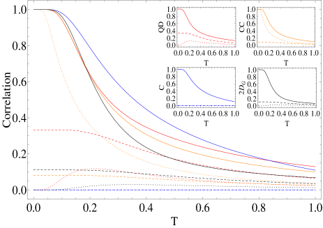
Figure 1: (Color online) Various correlations are plotted as a function of temperature $T$ for different isotropy $J$ with $J_{z}=-0.5$ in the absence of $B$ and $D$, in which $J=0.3,0.5,1$ corresponds to dotted, dashed and solid line respectively. QD, CC, C and GMD corresponds respecitvely to the red, orange, blue and black line. The inset is the uncombined plot.

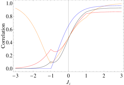
Figure 2: (Color online) Various correlations versus the anisotropy $J_{z}$ in the absence of B and D, with $J=1$, $T=0.5$. The red, orange, blue and black line indicates QD, CC, C and GMD respectively.

Subsequently, in order to demonstrate the effect of $J_{z}$ on various quantities, we plot Fig. 2, from which one can see that both QD and GMD are zero when $J_{z}$ is small in the negative region, and start to increase with the increasing of $J_{z}$ at the critical point until $J_{z}=-J=-1$, at which they undergo the so-called sudden change. With the further increase of $J_{z}$, they decrease slightly and then continue to increase until reaches two different stable values (near the maximum). Note that the sudden change also occurs at $J_{z}=J=1$ for both of them. However the above process is not true for C and CC. C is always null in the region $J_{z}<-1$ and begins to increase abruptly at $J_{z}=-1$ until to a stable value as $J_{z}$ increases and the sudden change does not happen for C. As for CC, it decreases from the maximum value to the minimum value as $J_{z}$ increases until $J_{z}=-1$ and undergoes the sudden change twice at $J_{z}=\pm J$, then finally revives to the maximum value with the further increase of $J_{z}$. Thereby, by comparing with the result in Ref. WerlangPRA2 that QD can signal a QPT at finite temperature while C can’t, we can conclude that not only QD (or GMD), but also CC can detect the critical points of QPT.

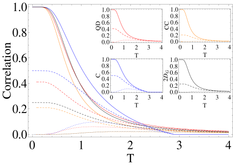
Figure 3: (Color online) Various correlations are plotted as a function of temperature $T$ for different magnetic field $B$ with $J_{z}=1$, $D=0$, where $B=0,2,4$ corresponds respectively to the solid, dashed and dotted line. The red, orange, blue and black line indicates QD, CC, C and GMD respectively. The inset is the uncombined plot.

Figures 3 and 5 are plotted to exhibit the ffects of $B$ and $D$ on various quantities as the external magnetic field and DM interaction are introduced. One can clearly see that $B$ plays a destructive role in the manipulation and control of these correlations from Fig. 3. But it still deserves to be studied since the introduction of it is sometime in practical need such as the nuclear magnetic resonance quantum computing and the superconducting quantum computing. In particular, the destructive effect of $B$ can be compensated through adjusting other tunable system parameters, say $J$ and $D$ for instance. In order to compare the efficiency of the parameters against the detrimental $B$, we plot the QD as a function of $B$ and $D$ (or $B$ and $J,$ or $B$ and $J_{z}$) in Fig. 4. The figure shows that the effects of $J$ and $D$ on QD are exactly equivalent and can tune QD to the maximal value as long as they are large enough, whereas the effect of $J_{z}$ is comparatively weaker (see the lower surface plot in Fig. 4) in compensating the detrimental influence of $B$ on QD. The behavior of other three quantities versus these system parameters are similar (plots omitted). Furthermore, we should note that the difference of these quantities becomes larger as $B$ increases until the critical value, at which these quantities start at zero and increase as temperature rises (i.e., the value of any quantity at zero temperature limit transits from nonnull to null at the critical magnetic field or vice versa). With the further increase of $B$, such difference vanishes. Moreover, as mentioned above in Fig. 1, QD increases with $T$ when $J_{z}$ is in the negative region. Such negative-only region can be widened to the positive one by the inclusion of a strong $B$, and also such characteristic is awarded to CC and C. Besides, Fig. 5 shows that DM interaction is constructive for various quantities. We should note that the difference of QD and CC becomes smaller as $D$ increases and the two curves overlap each other when $D$ is large enough, while the difference of QD and C becomes larger with $D$. However, QD and GMD almost overlap each other all the time and the influence of $D$ on their negligible distinction is very slight. In addition, $D$ as well as $J$ turn out to be the most efficient parameters in increasing various correlations as well as the critical temperature.

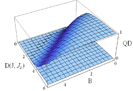
Figure 4: (Color online) The QD are plotted as a function of $B$ and $D$ (or $B$ and $J,$ or $B$ and $J_{z}$) at temperature $T=0.5$ with other parameters fixed at the value 0.1. The upper surface plot represents two completely overlapped surfaces QD($B,D$) and QD($B,J$), and the lower one corresponds to QD($B,J_{z}$).

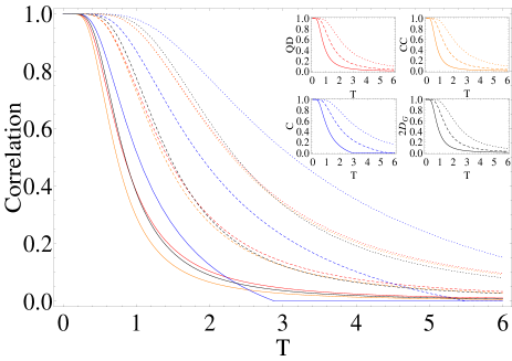
Figure 5: (Color online) Various correlations are plotted as a function of temperature $T$ for different $D$ with $J_{z}=1$, $B=0$, where $D=0,2,4$ corresponds respectively to the solid, dashed and dotted line. The red, orange, blue and black line indicates QD, CC, C and GMD respectively. The inset is the uncombined plot.

IV The correlations under the intrinsic decoherence

Now we consider the influence of intrinsic decoherence, proposed by Milburn MilburnPRA with the assumption that a system does not evolve continuously under unitary transformation for sufficiently short time steps, on various correlations. The master equation describing the intrinsic decoherence can be formulated as

$$\frac{d\rho(t)}{dt}=-i[H,\rho]-\frac{1}{2\gamma}[H,[H,\rho(t)]],$$ (20)

where $\gamma$ is the phase (intrinsic) decoherence rate. The formal solution of the above equation is given by CessaPRA

$$\rho(t)=\sum_{k=0}^{\infty}\frac{l^{k}}{k!}M^{k}(t)\rho(0)M^{\dagger k}(t),$$ (21)

where $\rho(0)$ is the density operator of the initial system and $M^{k}(t)$ is defined by

$$M^{k}(t)=H^{k}\exp(-\textrm{i}Ht)\exp\bigg{(}-\frac{t}{2\gamma}H^{2}\bigg{)}.$$ (22)

Then the time evolution of the density operator for the Heisenberg $XXZ$ spin system mentioned in the above section can be expressed by

$$\hskip 17.07164pt\rho(t)=\sum_{mn}\exp\bigg{[}-\frac{\gamma t}{2}(E_{m}-E_{n})^{2}-\textrm{i}(E_{m}-E_{n})t\bigg{]}\qquad$$

$$\qquad\times\langle\psi_{m}|\rho(0)|\psi_{n}\rangle|\psi_{m}\rangle\langle\psi_{n}|,$$ (23)

where $E_{m,n}$ and $\psi_{m,n}$ are the eigenvalues and the corresponding eigenvectors of the Hamiltonian respectively.

Firstly, we assume that the initial state of the system is $|\Psi_{1}(0)\rangle=\frac{1}{\sqrt{2}}\big{(}|01\rangle+|10\rangle\big{)}$ and then $\rho_{1}(0)=|\Psi_{1}(0)\rangle\langle\Psi_{1}(0)|$. Secondly, we consider another initial state $|\Psi_{2}(0)\rangle=\frac{1}{\sqrt{2}}\big{(}|00\rangle+|11\rangle\big{)}$. As per the Eqs. (1) $\sim$ (III) and (IV), after some algebras, one can obtain the analytical expressions for the dynamical behavior of various correlations as

$$\begin{array}[]{ll}C_{1}(t)=\mu^{-1}\sqrt{J^{2}+D^{2}e^{-4\mu^{2}\gamma t}\cos(2\mu t)},\\ QD_{1}(t)=-\sum\limits_{i=1}^{2}\alpha_{i}\log_{2}\alpha_{i}+\sum\limits_{i=3}^{4}\alpha_{i}\log_{2}\alpha_{i},\\ CC_{1}(t)=-\sum\limits_{i=1}^{2}\alpha_{i}\log_{2}\alpha_{i},\\ 2D_{G1}(t)=\frac{1}{2\mu^{2}}\big{[}2J^{2}+D^{2}e^{-4\mu^{2}\gamma t}\big{(}1+\cos^{2}(4\mu t)\big{)}\big{]},\\ \end{array}$$ (28)

for the initial state $|\Psi_{1}(0)\rangle$ and

$$\begin{array}[]{ll}C_{2}(t)=e^{-2B^{2}\gamma t},\\ QD_{2}(t)=1+\sum\limits_{i=1}^{2}\beta_{i}\log_{2}\beta_{i},\\ CC_{2}(t)=1,\\ 2D_{G2}(t)=e^{-4B^{2}\gamma t},\\ \end{array}$$ (33)

for the initial state $|\Psi_{2}(0)\rangle$, where $\alpha_{1,2}=\frac{1}{2}\big{[}1\pm\mu^{-1}De^{-2\mu^{2}\gamma t}\sin(2\mu t)\big{]}$, $\alpha_{3,4}=\frac{1}{2}\big{(}1\pm\mu^{-1}e^{-2\mu^{2}\gamma t}\sqrt{D^{2}+J^{2}e^{2\mu^{2}\gamma t}}\big{)}$, and $\beta_{1,2}=\frac{1}{2}\big{(}1\pm e^{-2B^{2}\gamma t}\big{)}$. From the analytical expressions, one can readily see that the time evolution of these quantities are independent of $J_{z}$ in both cases under consideration. Also, they are independent of $B$ in the case that the initial state is $|\Psi_{1}(0)\rangle$, whereas independent of $J$ and $D$ in the case that $|\Psi_{2}(0)\rangle$ is chosen as the initial state.

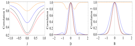
Figure 6: (Color online) Time evolution of various correlations are plotted as a function of $J$ (with $D=0.4$),$D$ (with $J=0$) and $B$ respectively at time $t=1$ with fixed decoherence rate $\gamma=1$, in which the orange, blue, black and red line corresponds to CC, C, GMD and QD respectively.

In what follows, we are dedicated to the numerical results. In Fig. 6 we plot the time evolution of various quantities versus $J,$ $D$ and $B$ respectively with other parameters fixed. From the figure one can see that the effects of $J$ and $B$ on the time evolution behavior of various quantities are similar to that in thermal equilibrium except that CC is always maximal and independent of $B$. However, the effect of $D$ on the dynamics of various correlations are notably different from its effect in thermal equilibrium. Note that $D$ is completely detrimental for QD and GMD and nearly destructive for C except for a process of sudden death and slight revival, while almost beneficial for CC apart from a so-called regrowth process that CC decreases to the minimum value (not zero) as $D$ increases and then increases to the maximal value.

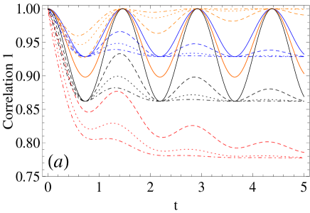
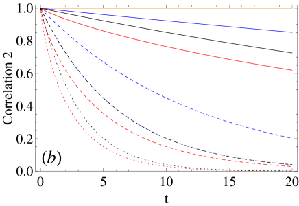
Figure 7: (Color online) Time evolution of various correlations are plotted as a function of time $t$ for different decoherence rate $\gamma$ with two different initial states, where $\gamma=0,0.1,0.2,0.3$ corresponds respectively to the solid, dashed, dotted and dot-dashed line in $(a)$, $\gamma=0.1,1,2$ corresponds to the solid, dashed and dotted line respectively in $(b)$. The orange, blue, black and red line represents CC, C, GMD and QD respectively.

Finally, Fig. 7 is plotted for the two different initial states in order to observe the effects of pure phase decoherence rate $\gamma$ on the dynamics of various quantities. Before giving the numerical analysis, we should clarify that the orange-solid line and red-solid line in (a) as well as the blue-dotted line and black-dashed line in (b) are fully overlapped. Figure 7(a) depicts that the dynamics of these quantities oscillate with time $t$ periodically with the same periodicity and the amplitudes of C, QD and GMD decay gradually to a stable value after a long time evolution as intrinsic decoherence is taken into account, while that of CC, on the contrary, is enhanced with the increase of $\gamma$. The larger $\gamma$ leads to the faster decay (or promotion for CC) in a short time. Furthermore, when $J=0$ and $\gamma$ is very small, these quantities undergo the sudden death and revival periodically. Figure 7(b) shows that CC is maximal all the time but other quantities dissipate monotonously and disappear eventually as time goes to infinity so that we can conclude that CC is robust against these tunable parameters whereas QD is most sensitive. Moreover, there is a descending order of CC, C, GMD and QD when the initial state is $|\Psi_{2}(0)\rangle$ with a nonnull $B$ (when $B=0$, these quantities are all maximal).

V Conclusion

In summary, we have investigated various correlations measured by C, CC, QD and GMD in a two-qubit Heisenberg $XXZ$ spin chain in the presence of external magnetic field and DM anisotropic antisymmetric interaction both in thermal equilibrium and under the intrinsic decoherence cases. We have obtained analytical expressions for these correlations for both cases and discussed their behaviors following various system parameters at length. The results show that the isotropy parameter $J$ plays a constructive role in the manipulation and control of various correlations and the anisotropy $J_{z}$ is considerably crucial for these quantities in thermal equilibrium at zero temperature limit but ineffective under the consideration of the intrinsic decoherence. When $J_{z}<J<-J_{z}$ ($J_{z}$ is negative) in the absence of $B$ and $D$, QD and GMD start at zero and increase as $T$ rises to a certain value, then decrease, while C is zero and CC declines from the maximal value with the rise of $T$. For $J=|J_{z}|$, all the quantities start at a certain value and decrease with $T$ except for C which is still zero. When $|J|>-J_{z}$, all quantities decrease starting from maximum with $T$. Therefore, $J_{z}=\pm J$ are the QPT points which are signaled not only by QD and GMD, but also by CC. As $B$ and $D$ are introduced to the system, the range of $J_{z},$ in which the quantities start at zero and increase with $T$ to a certain value then decrease, are widened to the positive region. The inclusion of $B$ turns out to be destructive, nevertheless it still deserves to be studied for its practical application in some implementations such as the nuclear magnetic resonance quantum computing and the superconducting quantum computing. $D$ plays a constructive role and the effects of $J$ and $D$ on the correlations are exactly equivalent and they turn out to be the most efficient in compensating the detrimental influence of $B$. Furthermore, the difference of various quantities becomes larger with the enhancement of $B$ until the critical point, after which it minifies. When the intrinsic decoherence is taken into account, the effect of $J$ and $B$ are similar with that in thermal equilibrium, but $D$ becomes to be destructive. In addition, the dynamics of these quantities oscillate with time $t$ when the initial state is $|\Psi_{1}(0)\rangle$ and the amplitudes of C, QD and GMD decay to a stable value after a long time evolution with the enhancement of $\gamma$, while that of CC, on the contrary, is enhanced with the increase of $\gamma$. And CC is maximal all the time but other quantities dissipate degressively and disappear eventually with $t$ when the initial state is chosen as an alternative Bell state $|\Psi_{2}(0)\rangle$. Moreover, there is not a definite ordering of various quantities in thermal equilibrium, whereas there is a descending order of CC, C, GMD and QD under the intrinsic decoherence with a nonnull $B$ when the initial state is chosen as $|\Psi_{2}(0)\rangle$.

- (1) M. A. Neilsen and I. L. Chuang, Quantum computation and quantum information (Cambridge University Press), Cambridge, UK, 2000.
- (2) C. H. Bennett, G. Brassard, C. Crépeau, R. Jozsa, A. Peres and W. K. Wootters, Phys. Rev. Lett. 70, 1895 (1993).
- (3) C. H. Bennett and S. J. Wiesner, Phys. Rev. Lett. 69, 2881 (1992).
- (4) A. K. Ekert, Phys. Rev. Lett. 67, 661 (1991).
- (5) S. L. Luo, Phys. Rev. A 77, 022301 (2008).
- (6) H. Ollivier and W. H. Zurek, Phys. Rev. Lett. 88, 017901 (2001).
- (7) B. P. Lanyon, M. Barbieri, M. P. Almeida, and A. G. White, Phys. Rev. Lett. 101, 200501 (2008).
- (8) A. Datta, A. Shaji, and C. M. Caves, Phys. Rev. Lett. 100, 050502 (2008).
- (9) S. L. Luo, Phys. Rev. A 77, 042303 (2008).
- (10) M. S. Sarandy, Phys. Rev. A 80, 022108 (2009).
- (11) T. Werlang, S. Souza, F. F. Fanchini, and C. J. Villas Boas, Phys. Rev. A 80, 024103 (2009).
- (12) M. Ali, A. R. P. Rau, and G. Alber, Phys. Rev. A 81, 042105 (2010).
- (13) T. Werlang, and G. Rigolin, Phys. Rev. A 81, 044101 (2010).
- (14) F. F. Fanchini, T. Werlang, C. A. Brasil, L. G. E. Arruda, and A. O. Caldeira, Phys. Rev. A 81, 052107 (2010).
- (15) Z. Y. Sun, L. Li, K. L. Yao, G. H. Du, J. W. Liu, B. Luo, N. Li, and H. N. Li, Phys. Rev. A 82, 032310 (2010).
- (16) S. L. Luo, and S. S. Fu, Phys. Rev. A 82, 034302 (2010).
- (17) L. Ciliberti, R. Rossignoli, and N. Canosa, Phys. Rev. A 82, 042316 (2010).
- (18) B. Q. Liu, B. Shao, and J. Zou, Phys. Rev. A 82, 062119 (2010).
- (19) Z. N. Li, J. S. Jin, and C. S. Yu, Phys. Rev. A 83, 012317 (2011).
- (20) B. Li, Z. X. Wang, and S. M. Fei, Phys. Rev. A 83, 022321 (2011).
- (21) A. Al-Qasimi, and D. F. V. James, Phys. Rev. A 83, 032101 (2011).
- (22) P. Parashar, and S. Rana, Phys. Rev. A 83, 032301 (2011).
- (23) D. Girolami, and G. Adesso, Phys. Rev. A 83, 052108 (2011).
- (24) R. Dillenschneider, Phys. Rev. B 78, 224413 (2008).
- (25) A. Shabani, and D. A. Lidar, Phys. Rev. Lett. 102, 100402 (2009).
- (26) M. D. Lang, and C. M. Caves, Phys. Rev. Lett. 105, 150501 (2010).
- (27) B. Dakić, V. Vedral, and Č. Brukner, Phys. Rev. Lett. 105, 190502 (2010).
- (28) A. Streltsov, H. Kampermann, and D. Bruß, Phys. Rev. Lett. 106, 160401 (2011).
- (29) J. B. Yuan, L. M. Kuang, and J. Q. Liao, J. Phys. B: At. Mol. Opt. Phys. 43, 165503 (2010).
- (30) Z. Sun, X. M. Lu, and L. J. Song, J. Phys. B: At. Mol. Opt. Phys. 43, 215504 (2010).
- (31) J. L. Guo, Y. J. Mi, J. Zhang and H. S. Song, J. Phys. B: At. Mol. Opt. Phys. 44, 065504 (2011).
- (32) X. M. Lu, Z. J. Xi, Z. Sun and X. G. Wang, Quantum Inf. Comput. 10, 0994 (2010).
- (33) J. S. Xu, X. Y. Xu, C. F. Li, C. J. Zhang, X. B. Zou and G. C. Guo, Nat. Commun. 1, 7 (2010).
- (34) J. Maziero, L. C. Céleri, R. M. Serra and V. Vedral, Phys. Rev. A 80, 044102 (2009).
- (35) J. Maziero, T. Werlang, F. F. Fanchini, L. C. Céleri, and R. M. Serra, Phys. Rev. A 81, 022116 (2010).
- (36) L. Mazzola, J. Piilo, and S. Maniscalco, Phys. Rev. Lett. 104, 200401 (2010).
- (37) B. Wang, Z. Y. Xu, Z. Q. Chen and M. Feng, Phys. Rev. A 81, 014101 (2010).
- (38) R. Vasile, P. Giorda, S. Olivares, M. G. A. Paris, and S. Maniscalco, Phys. Rev. A 82, 012313 (2010).
- (39) M. A. Nielsen, Phys. Rev. A 63, 022114 (2001).
- (40) X. G. Wang, Phys. Rev. A 64, 012313 (2001).
- (41) G. L. Kamta and A. F. Starace, Phys. Rev. Lett. 88, 107901 (2002).
- (42) K. M. O’Connor and W. K. Wootters, Phys. Rev. A 63, 052302 (2001).
- (43) Y. Sun, Y. G. Chen and H. Chen, Phys. Rev. A 68, 044301 (2003).
- (44) Y. Yeo, Phys. Rev. A 66, 062312 (2002).
- (45) A. Abliz, J. T. Cai, G. F. Zhang and G. S. Jin, J. Phys. B: At. Mol. Opt. Phys. 42, 215503 (2009).
- (46) J. T. Cai, A. Abliz, G. F. Zhang and Y. K. Bai, Opt. Commun. 283, 4415 (2010).
- (47) D. Loss, and D. P. DiVincenzo, Phys. Rev. A 57, 120 (1998).
- (48) G. Burkard, D. Loss, and D. P. DiVincenzo, Phys. Rev. B 59, 2070 (1999).
- (49) B. E. Kane, Nature 393, 133 (1998).
- (50) A. Sorensen, L. M. Duan, J. I. Cirac and P. Zoller, Nature, 409, 63 (2001).
- (51) W. M. Liu, W. B. Fan, W. M. Zheng, J. Q. Liang, and S. T. Chui, Phys. Rev. Lett. 88, 170408 (2002).
- (52) D. A. Lidar, D. Bacon and K. B. Whaley, Phys. Rev. Lett. 82, 4556 (1999).
- (53) D. P. DiVincenzo, D. Bacon, J. Kempe, G. Burkard and K. B. Whaley, Nature 408, 339 (2000).
- (54) L. F. Santos, Phys. Rev. A 67, 062306 (2003).
- (55) W. K. Wootters, Phys. Rev. Lett. 80, 2245 (1998).
- (56) T.M. Cover and J.A. Thomas, Elements of Information Theory (J. Wiley, New York, 1991).
- (57) A. Wehrl, Rev. Mod. Phys. 50, 221 (1978); V. Vedral, Rev. Mod. Phys. 74, 197 (2002).
- (58) I. Dzyaloshinskii, J. Phys. Chem. Solids. 4, 241 (1958).
- (59) T. Moriya, Phys. Rev. 120, 91 (1960).
- (60) G. J. Milburn, Phys. Rev. A 44, 5401 (1991).
- (61) H. Moya-Cessa, V. Bužek, M. S. Kim and P. L. Knight, Phys. Rev. A 48, 3900 (1993).