The Cost of Bounded Curvature

Abstract

We study the motion-planning problem for a car-like robot whose turning radius is bounded from below by one and which is allowed to move in the forward direction only (Dubins car). For two robot configurations $\sigma,\sigma^{\prime}$, let $\ell(\sigma,\sigma^{\prime})$ be the shortest bounded-curvature path from $\sigma$ to $\sigma^{\prime}$. For $d\geqslant 0$, let $\ell(d)$ be the supremum of $\ell(\sigma,\sigma^{\prime})$, over all pairs $(\sigma,\sigma^{\prime})$ that are at Euclidean distance $d$. We study the function $\operatorname{dub}(d)=\ell(d)-d$, which expresses the difference between the bounded-curvature path length and the Euclidean distance of its endpoints. We show that $\operatorname{dub}(d)$ decreases monotonically from $\operatorname{dub}(0)=7\pi/3$ to $\operatorname{dub}(d^{\ast})=2\pi$, and is constant for $d\geqslant d^{\ast}$. Here $d^{\ast}\approx 1.5874$. We describe pairs of configurations that exhibit the worst-case of $\operatorname{dub}(d)$ for every distance $d$.

1 Introduction

Motion planning or path planning involves computing a feasible path, possibly optimal for some criterion such as time or length, of a robot moving among obstacles; see the book by Lavalle [17] and book chapters by Halperin et al. [14] and Sharir [24]. A robot generally comes with physical limitations, such as bounds on its velocity, acceleration or curvature. Such differential constraints restrict the geometry of the paths the robot can follow. In this setting, the goal of motion planning is to find a feasible (or optimal) path satisfying both global (obstacles) and local (differential) constraints if it exists.

In this paper, we study the bounded-curvature motion planning problem which models a car-like robot. A car (with front-wheel steering) is constrained to move in the direction that the rear wheels are pointing, and it has a fixed maximum steering angle. This makes the car travel in a motion with fixed minimum turning radius, which means that the car must follow a curvature-constrained path. More precisely, we have the following robot model:

Robot model (Dubins car).

The robot is considered a rigid body that moves in the plane. A configuration of the robot is specified by both its location, a point in $\mathbb{R}^{2}$ (typically, the midpoint of the rear axle), and its orientation, or direction of travel. The robot is constrained to move in the forward direction, and its turning radius is bounded from below by a positive constant, which can be assumed to be equal to one by scaling the space. In this context, the robot follows a bounded-curvature path, that is, a differentiable curve whose curvature is constrained to be at most one almost everywhere.

Planning the motion of a car-like robot has received considerable attention in the literature. In this paper, we consider the cost of this restriction: How much longer is the shortest path made by such a robot compared to the Euclidean distance travelled?

Formally, consider two configurations $\sigma$ and $\sigma^{\prime}$. Let $\ell(\sigma,\sigma^{\prime})$ denote the length of a shortest curvature-constrained path from $\sigma$ to $\sigma^{\prime}$, and let $d(\sigma,\sigma^{\prime})$ denote the Euclidean distance between $\sigma$ and $\sigma^{\prime}$. We define

$$\operatorname{dub}(d) =\sup\{\ell(\sigma,\sigma^{\prime})-d\mid\text{$\sigma$, $\sigma^{\prime}$ configurations with $d(\sigma,\sigma^{\prime})=d$}\}.$$ (1)

Note that the supremum here is not a maximum, as the path length is not a continuous function of the orientations at the two endpoints. Our goal is to understand the function $\operatorname{dub}:\mathbb{R}\mapsto\mathbb{R}$ in detail. While this is a natural and fundamental question related to motion planning with bounded curvature, it is also a relevant question that has repeatedly appeared in the literature, with only partial answers so far.

Dubins [11] showed that the shortest curvature-constrained path between two configurations consists of at most three segments, each of which is either a straight segment or a circular arc of radius one. Using ideas from control theory, Boissonnat et al. [7], in parallel with Sussmann and Tang [26], gave an alternative proof. Sussmann [25] extended the characterization to the 3-dimensional case. Bui et al. [10] discussed how the types of optimal paths partition the configuration space, and also proved that optimal paths for free final orientation have at most two segments [6]. Significant work has been done on the problems of deciding whether a bounded-curvature path exists between given configurations among different kinds of obstacles and finding the shortest such path [12, 5, 21, 15, 3, 4, 2, 1, 9, 8].

At least two interesting problems have been studied where not configurations but only locations for the robot are given. The first problem considers a sequence of points in the plane, and asks for the shortest curvature-constrained path that visits the points in this sequence. In the second problem, the Dubins traveling salesman problem, the input is a set of points in the plane, and asks to find a shortest curvature-constrained path visiting all points. Both problems have been studied by researchers in the robotics community, giving heuristics and experimental results [22, 19, 20]. From a theoretical perspective, Lee et al. [18] gave a linear-time, constant-factor approximation algorithm for the first problem. No general approximation algorithms are known for the Dubins traveling salesman problem (the approximation factor of the known algorithms depends on the smallest distance between points).

All this work depends on some knowledge of the function $\operatorname{dub}$. Lee et al. [18], for instance, prove that the approximation ratio of their algorithms is $\max(\mathcal{A},\pi/2+\mathcal{B}/\pi)$, where $\mathcal{A}=1+\sup\{\operatorname{dub}(d)/d\mid d\geqslant 2\}$ and $\mathcal{B}=\sup\{\operatorname{dub}(d)+d\mid d\leqslant 2\}$. They claim without proof that $\operatorname{dub}(d)\leqslant 2\pi$ for $d\geqslant 2$ and derive from this that $\mathcal{A}=1+\pi$ and $\mathcal{B}\leqslant 5\pi/2+3$, leading to an approximation ratio of about $5.03$. We give the first proof of $\mathcal{A}=1+\pi$, and improve the second bound to $\mathcal{B}=2+2\pi$, improving the approximation ratio of their algorithm to $2+2/\pi+\pi/2\approx 4.21$.

Savla et al. [23] prove that $\operatorname{dub}(d)\leqslant\kappa\pi$, where $\kappa\in[2.657,2.658]$, and conjecture based on numerical experiments that the true bound is $7\pi/3$. We show that this is indeed true.

Results.

We show that $d\mapsto\operatorname{dub}(d)$ is a decreasing function with two breakpoints, at $\sqrt{2}$ and at $d^{\ast}\approx 1.5874$ (see Figure 1). More precisely, we have $\operatorname{dub}(0)=7\pi/3$ and the two breakpoint values are $\operatorname{dub}(\sqrt{2})=5\pi/2-\sqrt{2}$, and $\operatorname{dub}(d^{\ast})=2\pi$. The function $\operatorname{dub}(d)$ is constant and equal to $2\pi$ for $d\geqslant d^{\ast}$.

Figure 1: The graph of the function $\operatorname{dub}(d)$.

For $0\leqslant d<\sqrt{2}$ and for $d\geqslant d^{\ast}$, the supremum in (1) is in fact a maximum, and we give configurations $\sigma,\sigma^{\prime}$ at distance $d$ such that $\ell(\sigma,\sigma^{\prime})=\operatorname{dub}(d)+d$. Perhaps surprisingly, for $\sqrt{2}\leqslant d<d^{\ast}$, there are no such configurations—the supremum is not a maximum.

Our proof is long and contains calculations that some readers may find tedious. After laying the necessary groundwork in Section 2, we will therefore provide only a high-level proof in Section 3. We fill in the details in Sections 4 to 8, leaving some of the more technical or tedious calculations to an appendix.

2 Preliminaries

Notations.

For two points $P$ and $Q$, we denote by $\overline{PQ}$ the line segment with endpoints $P$ and $Q$, and by $\ddddot{PQ}$ an arc of unit radius with endpoints $P$ and $Q$. (If the length of $\overline{PQ}$ is less than two then there are four such arcs, so unless it is clear from the context, we will specify the supporting circle and the orientation of the arc.) We denote the length of the segment $\overline{PQ}$ as $|\overline{PQ}|$ or simply as $|PQ|$, and the length of the arc $\ddddot{PQ}$ as $|\ddddot{PQ}|$.

Without loss of generality, we assume that the starting configuration is $(0,0,\alpha)$—that is, we start at the origin $S=(0,0)$ with orientation $\alpha$—and the final configuration is $(d,0,\beta)$—that is, we arrive at $F=(d,0)$ with orientation $\beta$. Here, $\alpha$ and $\beta$ express the orientation of the robot as an angle with the positive $x$-axis, and $d\geqslant 0$ is the Euclidean distance of the two configurations.

The open unit (radius) disks tangent to the starting and final configurations are denoted $L_{S},R_{S},L_{F},R_{F}$, where the letters $L$ or $R$ depend on whether the disk is located on the left or right side of the direction vector (see Figure 2).

Figure 2: An example of a pair of configurations.

Let $\ell_{S},r_{S},\ell_{F},r_{F}$ denote the centers of $L_{S},R_{S},L_{F},R_{F}$, respectively. For future reference, we note their coordinates:

$$\ell_{S} =(\cos(\alpha+\pi/2),\sin(\alpha+\pi/2))=(-\sin\alpha,\cos\alpha)$$

$$r_{S} =(\cos(\alpha-\pi/2),\sin(\alpha-\pi/2))=(\sin\alpha,-\cos\alpha)$$

$$\ell_{F} =(d+\cos(\beta+\pi/2),\sin(\beta+\pi/2))=(d-\sin\beta,\cos\beta)$$

$$r_{F} =(d+\cos(\beta-\pi/2),\sin(\beta-\pi/2))=(d+\sin\beta,-\cos\beta).$$

Distances between centers.

The following distances will be frequently used:

$$d_{\text{\tiny L}} =|\ell_{S}\ell_{F}|=\sqrt{(d-\sin\beta+\sin\alpha)^{2}+(\cos\beta-\cos\alpha)^{2}}$$ (2)

$$d_{\text{\tiny R}} =|r_{S}r_{F}|=\sqrt{(d+\sin\beta-\sin\alpha)^{2}+(-\cos\beta+\cos\alpha)^{2}}$$ (3)

$$d_{\text{\tiny LR}} =|\ell_{S}r_{F}|=\sqrt{(d+\sin\beta+\sin\alpha)^{2}+(-\cos\beta-\cos\alpha)^{2}}$$ (4)

$$d_{\text{\tiny RL}} =|r_{S}\ell_{F}|=\sqrt{(d-\sin\beta-\sin\alpha)^{2}+(\cos\beta+\cos\alpha)^{2}}.$$ (5)

Dubins paths.

Dubins [11] showed that for two given configurations in the plane, shortest bounded-curvature paths consist of arcs of unit radius circles ($C$-segments) and straight line segments ($S$-segments); moreover, such shortest paths are of type $\mathit{CCC}$ or $\mathit{CSC}$, or a substring thereof. These types of paths are referred to as Dubins paths.

For given $d\geqslant 0$, $\alpha,\beta\in[0,2\pi]$, there are up to six types of Dubins paths. The two path types $\mathit{LSL}$ and $\mathit{RSR}$ use outer tangents—these path types exist for any choice of $d,\alpha,\beta$. The two path types $\mathit{LSR}$ and $\mathit{RSL}$ use inner tangents, and exist only when the corresponding disks are disjoint. In particular, $\mathit{LSR}$ exists if and only if $d_{\text{\tiny LR}}\geqslant 2$, and $\mathit{RSL}$ exists if and only if $d_{\text{\tiny RL}}\geqslant 2$. The remaining two path types $\mathit{LRL}$ and $\mathit{RLR}$ exist whenever there is a disk tangent to the two disks, and so $\mathit{LRL}$ exists if and only if $d_{\text{\tiny L}}\leqslant 4$, and $\mathit{RLR}$ exists if and only if $d_{\text{\tiny R}}\leqslant 4$.

Dubins showed that in $\mathit{LRL}$- and $\mathit{RLR}$-paths the middle circular arc has length larger than $\pi$. This implies that of the two unit radius disks tangent to $L_{S}$ and $L_{F}$, only one is a candidate for the middle arc of an $\mathit{LRL}$-path, and similar for $\mathit{RLR}$-paths.

For $d\geqslant 0$ and $0\leqslant\alpha,\,\beta\leqslant 2\pi$, we define $\operatorname{\textsc{lsl}}(d,\alpha,\beta)$ to be the length of the $LSL$-path from $(0,0,\alpha)$ to $(d,0,\beta)$. We define $\operatorname{\textsc{rsr}},\operatorname{\textsc{lsr}},\operatorname{\textsc{rsl}},\operatorname{\textsc{lrl}},\operatorname{\textsc{rlr}}$ similarly, defining the length to be $\infty$ if no path of that type exists. The length of the shortest bounded-curvature path from $S$ to $F$ is then

$$\ell(d,\alpha,\beta)=\min\big{\{}\operatorname{\textsc{lsl}}(d,\alpha,\beta),\operatorname{\textsc{rsr}}(d,\alpha,\beta),\operatorname{\textsc{lsr}}(d,\alpha,\beta),\operatorname{\textsc{rsl}}(d,\alpha,\beta),\operatorname{\textsc{lrl}}(d,\alpha,\beta),\operatorname{\textsc{rlr}}(d,\alpha,\beta)\big{\}},$$

and our goal is to bound $\operatorname{dub}(d)=\sup_{0\leqslant\alpha,\beta\leqslant 2\pi}\ell(d,\alpha,\beta)-d$. (Note that the supremum here is not always a maximum as the function $\ell$ is not continuous.)

We will often suppress the argument $d$ for these functions when the distance $d$ is fixed and understood.

Monotonicity of the Dubins cost function.

Let $\square=[0,2\pi]^{2}$ denote the range of $(\alpha,\beta)$. Consider two distances $d_{1}<d_{2}$ and $(\alpha,\beta)\in\square$, and assume that we have a bounded-curvature path from $(0,0,\alpha)$ to $(d_{1},0,\beta)$ of length $\ell\leqslant\operatorname{dub}(d_{1})+d_{1}$. If this path has a horizontal tangent where the path is oriented to the right (in the direction of the positive $x$-axis), then we can insert a horizontal segment of length $d_{2}-d_{1}$ at this point, and obtain a path from $(0,0,\alpha)$ to $(d_{2},0,\beta)$ of length $\ell+(d_{2}-d_{1})\leqslant\operatorname{dub}(d_{1})+d_{2}$. See, for instance, Figure 3(a).

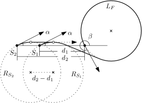
(a) $\ell(d_{2},\alpha,\beta)\leqslant\operatorname{\textsc{rsl}}(d_{1},\alpha,\beta)+(d_{2}-d_{1})$.

(b) An $\mathit{RLR}$-path that does not have a right horizontal tangent.

Figure 3: (a) Monotonicity of the length function of $\mathit{CSC}$-paths; (b) Non-monotonicity of the length function of $\mathit{CCC}$-path.

If this was possible for all $(\alpha,\beta)\in\square$, then it would imply that $\operatorname{dub}(d_{2})\leqslant\operatorname{dub}(d_{1})$, and it would follow that the Dubins cost function is monotone. Unfortunately, not all Dubins paths have horizontal tangents with the correct orientation (see Figure 3(b) for an example), and so proving the monotonicity of the Dubins cost function will require much more work. However, we can start with the following lemma:

Lemma 1.

Let $d_{1}<d_{2}$, and $(\alpha,\beta)\in\square$. If there is a path of length $\ell$ of type $\mathit{RSR}$, $\mathit{LSL}$, $\mathit{LSR}$, or $\mathit{RSL}$ from $(0,0,\alpha)$ to $(d_{1},0,\beta)$, then there is a path of length $\ell+(d_{2}-d_{1})$ from $(0,0,\alpha)$ to $(d_{2},0,\beta)$.

Proof.

It suffices to show that any of these path types must have a horizontal tangent oriented in the positive $x$-direction. By symmetry, it suffices to show this for $\mathit{RSR}$- and $\mathit{RSL}$-paths. The topmost point on a $\mathit{RSR}$-path necessarily has the correct tangent, so consider an $\mathit{RSL}$-path. It consists of a right-turning arc $\ddddot{ST_{1}}$ on $R_{S}$, a segment $\overline{T_{1}T_{2}}$, and a left-turning arc $\ddddot{T_{2}F}$ on $L_{F}$. If $\ddddot{ST_{1}}$ contains the topmost point of $R_{S}$, or if $\ddddot{T_{2}F}$ contains the bottommost point of $L_{F}$, these have the correct tangent, and we are done. Otherwise the path cannot possibly reach the positive $x$-axis, a contradiction. ∎

Symmetries.

For a fixed $d\geqslant 0$, determining $\operatorname{dub}(d)$ essentially amounts to finding $(\alpha,\beta)\in\square$ maximizing $\ell(\alpha,\beta)$ (“essentially” since the maximum may not actually be assumed). We now observe that the function $\ell(\alpha,\beta)$ has two symmetries.

First, we can mirror a path around the $x$-axis. This maps $\alpha$ to $-\alpha$, $\beta$ to $-\beta$, left disks to right disks, and right disks to left disks. As a result, we have, say, $\operatorname{\textsc{lsr}}(d,\alpha,\beta)=\operatorname{\textsc{rsl}}(d,-\alpha,-\beta)$, and in general we have $\ell(d,\alpha,\beta)=\ell(d,-\alpha,-\beta)$. See Figure 4.

Second, we can mirror a path around the line $x=d/2$ and reverse the direction of the path. If the original path connected $(0,0,\alpha)$ with $(d,0,\beta)$, the new path connects $(0,0,2\pi-\beta)$ to $(d,0,2\pi-\alpha)$. The transformation maps left disks to left disks and right disks to right disks, so we have, for instance $\operatorname{\textsc{lsr}}(d,\alpha,\beta)=\operatorname{\textsc{lsr}}(d,2\pi-\beta,2\pi-\alpha)$, and in general $\ell(d,\alpha,\beta)=\ell(d,2\pi-\beta,2\pi-\alpha)$. See Figure 5.

(a) Original path

(b) Mirrored along $x$-axis

(c) Point symmetry in $(\pi,\pi)$

Figure 4: Symmetry by mirroring the path along the $x$-axis.

(a) Original path

(b) Mirrored along the line $x=d/2$ while reversing the direction

(c) Reflection around the line $\beta=2\pi-\alpha$

Figure 5: Symmetry by mirroring the path along the line $x=d/2$ while reversing the direction.

Considered as symmetries on $\square$, the mapping $(\alpha,\beta)\mapsto(-\alpha,-\beta)$ is a point symmetry in $(\pi,\pi)$, while the mapping $(\alpha,\beta)\mapsto(2\pi-\beta,2\pi-\alpha)$ is a reflection around the line $\beta=2\pi-\alpha$.

It follows that $\sup_{(\alpha,\beta)\in[0,2\pi]^{2}}\ell(d,\alpha,\beta)=\sup_{(\alpha,\beta)\in\Delta}\ell(d,\alpha,\beta)$, where $\Delta$ is the triangle with corners $(0,0)$, $(\pi,\pi)$, and $(0,2\pi)$, or in other words the region

$$\Delta:\quad 0\leqslant\alpha\leqslant\pi\quad\text{and}\quad\alpha\leqslant\beta\leqslant 2\pi-\alpha.$$

In the following we will thus be able to restrict our considerations to the triangle $\Delta$ (see Figure 6(a)).

A new parameterization.

We now introduce a new parameterization of the $(\alpha,\beta)$-plane, which will sometimes be more convenient to work with:

$$\sigma=\frac{\beta+\alpha}{2},\quad\delta=\frac{\beta-\alpha}{2}.$$

In other words, we have

$$\alpha=\sigma-\delta,\quad\beta=\sigma+\delta.$$

Recall our triangle $\Delta$ from above. In the $(\sigma,\delta)$-representation, the triangle $\Delta$ is the triangle

$$\Delta:\quad 0\leqslant\sigma\leqslant\pi\quad\text{and}\quad 0\leqslant\delta\leqslant\sigma,$$

or the bottom right half of the square $\Gamma=[0,\pi]^{2}$ (see Figure 6(b)). In this representation, our first symmetry maps $(\sigma,\delta)$ to $(-\sigma,-\delta)$, while the second symmetry maps $(\sigma,\delta)$ to $(-\sigma,\delta)$. We thus have point symmetry in the origin, as well as mirror symmetry around the $\delta$-axis. In addition, $(\sigma+\pi,\delta+\pi)$ represents the same angles as $(\sigma,\delta)$ since $\alpha=\sigma-\delta$ and $\beta=\sigma+\delta$, and so we also have point symmetry in the point $(\pi/2,\pi/2)$, or in other words $\ell(d,\sigma,\delta)=\ell(d,\pi-\sigma,\pi-\delta)$.

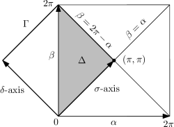
(a) $(\alpha,\beta)$-representation

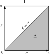
(b) $(\sigma,\delta)$-representation

Figure 6: $\Delta$ in two different representations.

Distances between centers (using $\sigma$ and $\delta$).

The following lemma will allow us to express the center distances in terms of $\sigma$ and $\delta$:

Lemma 2.

Let $d\geqslant 0$, and define the points $p(\vartheta)=(\cos\vartheta,\sin\vartheta)$ and $q(\vartheta)=(d-\cos\vartheta,\sin\vartheta)$ on the unit radius disks around $(0,0)$ and $(d,0)$. Then

$$|p(\vartheta-\phi)q(\vartheta+\phi)|^{2}=d^{2}-4d\cos\vartheta\cos\phi+4\cos^{2}\vartheta.$$

Proof.

We have

$$|p(\vartheta-\phi)q(\vartheta+\phi)|^{2} =\big{(}\cos(\vartheta-\phi)-d+\cos(\vartheta+\phi)\big{)}^{2}+\big{(}\sin(\vartheta-\phi)-\sin(\vartheta+\phi)\big{)}^{2}$$

$$=(\cos\vartheta\cos\phi+\sin\vartheta\sin\phi-d+\cos\vartheta\cos\phi-\sin\vartheta\sin\phi)^{2}$$

$$\mathrel{\phantom{=}}{}+(\sin\vartheta\cos\phi-\cos\vartheta\sin\phi-\sin\vartheta\cos\phi-\cos\vartheta\sin\phi)^{2}$$

$$=(2\cos\vartheta\cos\phi-d)^{2}+4\cos^{2}\vartheta\sin^{2}\phi$$

$$=d^{2}-4d\cos\vartheta\cos\phi+4\cos^{2}\vartheta\cos^{2}\phi+4\cos^{2}\vartheta\sin^{2}\phi$$

$$=d^{2}-4d\cos\vartheta\cos\phi+4\cos^{2}\vartheta.\qed$$

Lemma 2 leads to the following expressions for the squared distances between our disk centers:

$$d_{\text{\tiny L}}^{2} =|\ell_{S}\ell_{F}|^{2}=d^{2}-4d\sin\delta\cos\sigma+4\sin^{2}\delta$$ (6)

$$d_{\text{\tiny R}}^{2} =|r_{S}r_{F}|^{2}=d^{2}+4d\sin\delta\cos\sigma+4\sin^{2}\delta$$ (7)

$$d_{\text{\tiny LR}}^{2} =|\ell_{S}r_{F}|^{2}=d^{2}+4d\cos\delta\sin\sigma+4\cos^{2}\delta$$ (8)

$$d_{\text{\tiny RL}}^{2} =|r_{S}\ell_{F}|^{2}=d^{2}-4d\cos\delta\sin\sigma+4\cos^{2}\delta$$ (9)

To see this, observe that $\ell_{S}=p(\alpha+\pi/2)$, $r_{S}=p(\alpha-\pi/2)$, $\ell_{F}=q(\pi/2-\beta)$, and $r_{F}=q(3\pi/2-\beta)$. For $d_{\text{\tiny L}}$, set $\vartheta=\pi/2-\delta$, $\phi=-\sigma$; for $d_{\text{\tiny R}}$, set $\vartheta=\pi/2-\delta$, $\phi=\pi-\sigma$; for $d_{\text{\tiny LR}}$, set $\vartheta=\pi-\delta$, $\phi=\pi/2-\sigma$; for $d_{\text{\tiny RL}}$, set $\vartheta=-\delta$, $\phi=\pi/2-\sigma$.

The case $d=0$.

We first argue that $\operatorname{dub}(0)=7\pi/3$. The case $d=0$ is much easier since there is only one degree of freedom: Without loss of generality we can assume $\alpha=0$. It is easy to verify that for any $\beta$ there is a $\mathit{CCC}$-path of length at most $7\pi/3$. For $\beta=\pi$, no Dubins path has length shorter than $7\pi/3$, and so $\operatorname{dub}(0)=7\pi/3$ (see Figure 7). In the rest of this paper we can therefore mostly assume $d>0$, and avoid some degeneracies.

Figure 7: For $d=0$, $\alpha=0$ and $\beta=\pi$, we have $\operatorname{\textsc{lrl}}(d,\alpha,\beta)=\operatorname{\textsc{rlr}}(d,\alpha,\beta)={7\pi}/{3}$.

3 The overall proof

We subdivide the pairs of orientations $(\alpha,\beta)\in\Gamma$ into three cases. The case distinction is based on the existence of the $\mathit{LSR}$-path and the $\mathit{RSL}$-path:

• When neither the $\mathit{LSR}$-path nor the $\mathit{RSL}$-path exists, then we are in case A;

• when the $\mathit{RSL}$-path exists, but the $\mathit{LSR}$-path does not exist, then we are in case B; and

• when the $\mathit{LSR}$-path exists, then we are in case C.

The reader may wonder why the case distinction is not symmetric. We already broke the symmetry when we restricted our investigation to the triangle $\Delta$.

The $\mathit{LSR}$-path exists if and only if the disks $L_{S}$ and $R_{F}$ are disjoint (since the disks are open, they may touch, but cannot overlap), or, equivalently, if $|\ell_{S}r_{F}|=d_{\text{\tiny LR}}(\alpha,\beta)\geqslant 2$. The $\mathit{RSL}$-path exists if and only if $R_{S}$ and $L_{F}$ are disjoint, that is if $|r_{S}\ell_{F}|=d_{\text{\tiny RL}}(\alpha,\beta)\geqslant 2$. We can thus define three regions of the square $\Gamma$ for the three cases:

$$A =\{(\alpha,\beta)\in\Gamma\mid d_{\text{\tiny LR}}(\alpha,\beta)<2\;\text{and}\;d_{\text{\tiny RL}}(\alpha,\beta)<2\},$$

$$B =\{(\alpha,\beta)\in\Gamma\mid d_{\text{\tiny LR}}(\alpha,\beta)<2\;\text{and}\;d_{\text{\tiny RL}}(\alpha,\beta)\geqslant 2\},$$

$$C =\{(\alpha,\beta)\in\Gamma\mid d_{\text{\tiny LR}}(\alpha,\beta)\geqslant 2\}.$$

Figure 8 shows the subdivision of $\Gamma$ into the three regions for three different distances $d$.

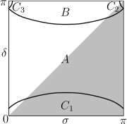
(a) $d=0.4$

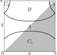
(b) $d=1.4$

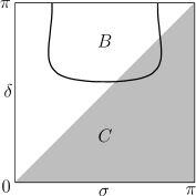
(c) $d=2.4$

Figure 8: Regions of cases A, B and C in $\Gamma$

It will be convenient to also define the parts of $A$, $B$ and $C$ that lie inside the triangle $\Delta$:

$$A^{\Delta}=A\cap\Delta,\quad B^{\Delta}=B\cap\Delta,\quad\text{and}\quad C^{\Delta}=C\cap\Delta.$$

We can now restrict the Dubins cost function $\operatorname{dub}(d)$ to the three regions

$$\operatorname{dub}_{A}(d) =\sup\nolimits_{(\alpha,\beta)\in A^{\Delta}}\ell(d,\alpha,\beta)-d$$

$$\operatorname{dub}_{B}(d) =\sup\nolimits_{(\alpha,\beta)\in B^{\Delta}}\ell(d,\alpha,\beta)-d$$

$$\operatorname{dub}_{C}(d) =\sup\nolimits_{(\alpha,\beta)\in C^{\Delta}}\ell(d,\alpha,\beta)-d$$

and we have

$$\operatorname{dub}(d) =\max\{\,\operatorname{dub}_{A}(d),\;\operatorname{dub}_{B}(d),\;\operatorname{dub}_{C}(d)\,\}.$$

Case C.

This is the easiest case, and we discuss it first in Section 4. Since both $\mathit{RSR}$- and $\mathit{LSR}$-paths exist, we can show that for $(\alpha,\beta)\in C^{\Delta}$ the $\mathit{RSR}$-path or the $\mathit{LSR}$-path has length at most $d+2\pi$ (Lemma 4). This implies that $\operatorname{dub}_{C}(d)\leqslant 2\pi$. The bound is tight, as the shortest path from configuration $(0,0,\pi)$ to $(d,0,\pi)$ has length $d+2\pi$ (Lemma 5), and so $\operatorname{dub}_{C}(d)=2\pi$. This implies a lower bound on the Dubins cost function: $\operatorname{dub}(d)\geqslant\operatorname{dub}_{C}(d)=2\pi$.

Case A.

We first observe that case A occurs only for $d<2$, as we have $8>d_{\text{\tiny LR}}^{2}+d_{\text{\tiny RL}}^{2}=2d^{2}+8\cos^{2}\delta\geqslant 2d^{2}$. In this case, neither $\mathit{LSR}$- nor $\mathit{RSL}$-paths exist. Since $|\ell_{S}\ell_{F}|\leqslant|\ell_{S}S|+|SF|+|F\ell_{F}|=d+2<4$ and $|r_{S}r_{F}|\leqslant|r_{S}S|+|SF|+|Fr_{F}|=d+2<4$, both $\mathit{LRL}$-path and $\mathit{RLR}$-path exist everywhere in $\Gamma$ for $d<2$.

It follows that the path types in case A are $\mathit{RSR}$, $\mathit{LSL}$, $\mathit{LRL}$, and $\mathit{RLR}$. It turns out that the shortest path is always of type $\mathit{CCC}$ (Lemma 18), and so we can concentrate entirely on comparing $\operatorname{\textsc{lrl}}(\alpha,\beta)$ and $\operatorname{\textsc{rlr}}(\alpha,\beta)$. To this end, we derive explicit expressions for the length of $\mathit{CCC}$-paths in Section 6. We examine the derivatives of these functions and show that they are monotone in $\sigma$- and $\delta$-directions (Lemma 13). Using monotonicity and Lagrange-multipliers, we show that $\operatorname{dub}_{A}(d)=\sup_{(\sigma,\delta)\in A}\ell(d,\sigma,\delta)-d$ is realized at a point $(\sigma_{A},\delta_{A})$ on the boundary of the region $A$ (Lemma 15).

For $0<d<\sqrt{2}$, this point is the unique point $(\pi,\delta_{A})\in A$ where $\operatorname{\textsc{lrl}}(\pi,\delta_{A})=\operatorname{\textsc{rlr}}(\pi,\delta_{A})$ (Lemma 19). For $\sqrt{2}\leqslant d<2$, however, the supremum $\sup_{(\sigma,\delta)\in A}\ell(d,\sigma,\delta)$ occurs on the common boundary of regions $A$ and $B$. Since this boundary belongs to region $B$, we can conclude that for $\sqrt{2}<d<2$ we have $\operatorname{dub}_{A}(d)\leqslant\max\{2\pi,\operatorname{dub}_{B}(d)\}$ (Lemma 20).

Case B.

In case B, the $\mathit{RSL}$-path exists, while the $\mathit{LSR}$-path does not exist. We have $|\ell_{S}\ell_{F}|\leqslant|\ell_{S}r_{F}|+|r_{F}\ell_{F}|=d_{\text{\tiny LR}}+2<4$, and so the $\mathit{LRL}$-path exists. We show that the shortest Dubins path is either the $\mathit{LRL}$-path or the $\mathit{RSL}$-path (Lemma 22).

The following lemma shows that case B occurs only in the upper half of the square $\Gamma$:

Lemma 3.

A point $(\sigma,\delta)\in B$ has $\delta>\pi/2$, and for $(\alpha,\beta)\in B^{\Delta}$ we have

$$0\leqslant\alpha\leqslant\pi/2\quad\text{and}\quad\pi+\alpha<\beta<2\pi-\alpha.$$ (10)

Proof.

$(\sigma,\delta)\in B$ means $d_{\text{\tiny LR}}^{2}<4$ and $d_{\text{\tiny RL}}^{2}\geqslant 4$, so $0>d_{\text{\tiny LR}}^{2}-d_{\text{\tiny RL}}^{2}=8d\cos\delta\sin\sigma$. Since $\sin\sigma\geqslant 0$, we must have $\cos\delta<0$, and thus $\delta>\pi/2$. So $(\sigma,\delta)$ lies in the top half of $\Gamma$. This top half intersects the triangle $\Delta$ in the triangle with corners (in $(\alpha,\beta)$-coordinates) $(0,\pi)$, $(\pi/2,3\pi/2)$, and $(0,2\pi)$, implying the claim. ∎

The function $\operatorname{\textsc{rsl}}(\alpha,\beta)$ was studied by Goaoc et al. [13], who gave an explicit expression for its derivative. We exploit this to show monotonicity of $\operatorname{\textsc{rsl}}(\alpha,\beta)$ (Lemma 21).

For $0<d<\sqrt{2}$, monotonicity of $\operatorname{\textsc{rsl}}(\alpha,\beta)$ easily implies the following proposition:

Proposition 1.

For $0<d<\sqrt{2}$, $\operatorname{dub}(d)=\operatorname{dub}_{A}(d)$. The function decreases monotonically from $\operatorname{dub}(0)=7\pi/3$ to $\operatorname{dub}(\sqrt{2})=5\pi/2-\sqrt{2}$.

Proof.

Let $0<d<\sqrt{2}$. By Lemma 19, $\operatorname{dub}_{A}(d)>2\pi+2\alpha^{\ast}-d$, and by the last statement of Lemma 21 we have $\operatorname{dub}_{B}(d)\leqslant 2\pi+2\alpha^{\ast}-d$ (here, $\alpha^{\ast}=\arcsin(d/2)$). Lemmas 19 and 16 imply that $\operatorname{dub}_{A}(d)$ decreases monotonically from $\operatorname{dub}_{A}(0)=7\pi/3$ to $\operatorname{dub}_{A}(\sqrt{2})=5\pi/2-\sqrt{2}$, and so $\operatorname{dub}_{A}(d)>2\pi=\operatorname{dub}_{C}(d)$. ∎

For $\sqrt{2}\leqslant d<2$, we are able to show that under the assumption that $\operatorname{dub}_{B}(d)>2\pi$, the value $\operatorname{dub}_{B}(d)$ is assumed at the (unique) point $(\alpha_{B},\beta_{B})$ on the common boundary of $B^{\Delta}$ and $C^{\Delta}$ where $\operatorname{\textsc{rsl}}(\alpha_{B},\beta_{B})=\operatorname{\textsc{lrl}}(\alpha_{B},\beta_{B})$ (Lemma 25). This common boundary, however, is part of the region $C^{\Delta}$. A shorter $\mathit{LSR}$-path exists in $C^{\Delta}$, and in fact there is no $(\alpha,\beta)\in B^{\Delta}$ with $\ell(d,\alpha,\beta)=\operatorname{dub}_{B}(d)+d$. We show that $\operatorname{dub}_{B}(d)$ is a monotonically decreasing function (Lemma 26), starting with $\operatorname{dub}_{B}(\sqrt{2})=\operatorname{dub}_{A}(\sqrt{2})=5\pi/2-\sqrt{2}$. Continuity and monotonicity imply that there is a distance $d^{\ast}$ where $\operatorname{dub}_{B}(d^{\ast})=2\pi$. We numerically computed $d^{\ast}\approx 1.5874$, and have the following proposition.

Proposition 2.

For $\sqrt{2}\leqslant d<d^{\ast}$, $\operatorname{dub}(d)=\operatorname{dub}_{B}(d)$. The function $\operatorname{dub}(d)$ decreases monotonically from $\operatorname{dub}_{B}(\sqrt{2})=5\pi/2-\sqrt{2}$ to $\operatorname{dub}(d^{\ast})=2\pi$. For $d^{\ast}\leqslant d<2$, $\operatorname{dub}(d)=2\pi$.

Proof.

By Lemma 20, we have $\operatorname{dub}_{A}(d)\leqslant\max\{2\pi,\operatorname{dub}_{B}(d)\}=\max\{\operatorname{dub}_{C}(d),\operatorname{dub}_{B}(d)\}$, and so $\operatorname{dub}(d)=\max\{2\pi,\operatorname{dub}_{B}(d)\}$. By Lemma 26 we have $\operatorname{dub}_{B}(d)>2\pi$ for $\sqrt{2}\leqslant d<d^{\ast}$. ∎

The case $d\geqslant 2$.

Propositions 1 and 2 describe the function $\operatorname{dub}(d)$ for $0\leqslant d<2$. It remains to prove that $\operatorname{dub}(d)=2\pi$ for $d\geqslant 2$, which amounts to analyzing $\operatorname{dub}_{B}(d)$. As shown in Figure 8, the region $B$ has a rather different shape for $d>2$, and our previous arguments do not carry over without additional tedious calculations.

Fortunately, monotonicity comes to the rescue. By Proposition 2 we have $\operatorname{dub}(d)=2\pi$ for $d^{\ast}\leqslant d<2$. We had seen in Lemma 1 that monotonicity holds when the original path is a $\mathit{CSC}$-path. In Lemma 11 we extend this lemma by including the $\mathit{LRL}$-path, at least when the configuration is in case $B^{\Delta}$. This allows us to prove the claim for $d\geqslant 2$.

Proposition 3.

For $d\geqslant 2$, we have $\operatorname{dub}(d)=2\pi$.

Proof.

Let $d\geqslant 2$ and $(\alpha,\beta)\in\Delta$. We need to show that $\ell(d,\alpha,\beta)\leqslant 2\pi+d$. If $(\alpha,\beta)\in C^{\Delta}$, then this follows from Lemma 4. Otherwise we must have $(\alpha,\beta)\in B^{\Delta}$, and we have $\delta>\pi/2$ by Lemma 3. We choose $d_{1}<2$ such that $d_{1}>2\sin(\pi-\delta)$ and $d_{1}>d^{\ast}$ and consider the configuration $(\alpha,\beta)$ for distance $d_{1}$. Since case A occurs only within the $\delta$-range $\arcsin(d_{1}/2)\leqslant\delta\leqslant\pi-\arcsin(d_{1}/2)$ (Lemma 6), we must be in either case B or case C, so there is a path of type $\mathit{RSR}$, $\mathit{LSR}$, $\mathit{RSL}$, or $\mathit{LRL}$ of length at most $d_{1}+\operatorname{dub}(d_{1})=d_{1}+2\pi$ from $(0,0,\alpha)$ to $(d_{1},0,\beta)$. By Lemmas 1 and 11 there is then a path from $(0,0,\alpha)$ to $(d,0,\beta)$ of length at most $d_{1}+2\pi+(d-d_{1})=d+2\pi$. ∎

Main result.

We summarize some of our results in the following theorem:

Theorem 1.

The function $\operatorname{dub}(d)$ has two breakpoints at $\sqrt{2}$ and $d^{\ast}\approx 1.5874$. For $d<\sqrt{2}$, $\operatorname{dub}(d)=\operatorname{dub}_{A}(d)\leqslant\operatorname{dub}_{A}(0)={7\pi}/{3}$. For $\sqrt{2}\leqslant d<d^{\ast}$, $\operatorname{dub}(d)=\operatorname{dub}_{B}(d)\leqslant\operatorname{dub}_{B}(\sqrt{2})={5\pi}/{2}-\sqrt{2}$. For $d\geqslant d^{\ast}$, we have $\operatorname{dub}(d)=2\pi$.

4 Case C

Both the $\mathit{RSR}$-path and the $\mathit{LSR}$-path exist in case C, and we show that at least one of them has length at most $d+2\pi$. The arguments presented here are already in Kim’s master thesis [16].

Lemma 4.

For $(\alpha,\beta)\in C^{\Delta}$, we have $\ell(d,\alpha,\beta)\leqslant 2\pi+d$.

Proof.

Since $L_{S}\cap R_{F}=\emptyset$, the starting point $S=(0,0)$ does not lie in $R_{F}$, and so there is a tangent to $R_{F}$ through $S$ that touches $R_{F}$ from above. Let $\alpha_{\text{\tiny SR}}$ be the angle made by this tangent and the positive $x$-axis (see Figure 9(a)).

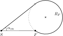
(a) Definition of $\alpha_{\text{\tiny SR}}$

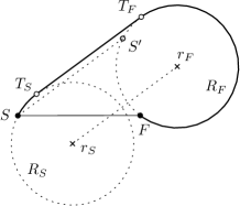
(b) $\mathit{RSR}$-path

Figure 9: $\mathit{RSR}$-paths in case C.

Let us first assume that $\alpha\geqslant\alpha_{\text{\tiny SR}}$, and consider the $\mathit{RSR}$-path from $S$ to $F$. It consists of an initial right-turning arc $\ddddot{ST_{S}}$, a straight line segment $\overline{T_{S}T_{F}}$, and a final right-turning arc $\ddddot{T_{F}F}$, where the segment is tangent to $R_{S}$ and $R_{F}$ at the points $T_{S}$ and $T_{F}$. (When $\alpha=\alpha_{\text{\tiny SR}}$ we have $S=T_{S}$.) See Figure 9.

Let $t$ be the vector $t=\overrightarrow{T_{S}T_{F}}$, and let $S^{\prime}=S+t$. Since $t=\overrightarrow{r_{S}r_{F}}$, we have $R_{F}=R_{S}+t$, and so $S^{\prime}$ lies on $R_{F}$. We claim that $S^{\prime}$ lies on the clockwise arc $\ddddot{FT_{F}}$. Indeed, any point $(\alpha,\beta)\in\Delta$ satisfies $\beta\leqslant\alpha\leqslant 2\pi-\beta$, which implies that $t$ has a positive $y$-component.

It follows that the length of the $\mathit{RSR}$-path is $|\ddddot{ST_{S}}|+|T_{S}T_{F}|+|\ddddot{T_{F}F}|=|SS^{\prime}|+|\ddddot{S^{\prime}F}|$. By the triangle-inequality, $|SS^{\prime}|\leqslant|SF|+|\ddddot{FS^{\prime}}|$, and so the length of the $\mathit{RSR}$-path is at most $|SF|+2\pi=d+2\pi$.

Consider now the case where $\alpha<\alpha_{\text{\tiny SR}}$. We show that the $\mathit{LSR}$-path from $S$ to $F$ has length at most $d+2\pi$. The $\mathit{LSR}$-path consists of an initial left-turning arc $\ddddot{ST_{S}}$, a straight line segment $\overline{T_{S}T_{F}}$ and a final right-turning arc $\ddddot{T_{F}F}$, where the segment is tangent to $L_{S}$ and $R_{F}$ at points $T_{S}$ and $T_{F}$. See Figure 10.

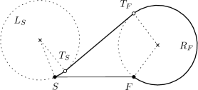
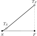
Figure 10: $\mathit{LSR}$-paths in case C.

Here, it suffices to observe that $|\ddddot{ST_{S}}|+|T_{S}T_{F}|\leqslant|SF|+|FT_{F}|$ (a convex curve contained within another convex curve), and so $|\ddddot{ST_{S}}|+|T_{S}T_{F}|+|\ddddot{T_{F}F}|\leqslant|SF|+|FT_{F}|+|\ddddot{T_{F}F}|\leqslant|SF|+|\ddddot{FT_{F}}|+|\ddddot{T_{F}F}|=d+2\pi$. ∎

It turns out that the bound in Lemma 4 is tight, and we obtain:

Lemma 5.

For any $d>0$ we have $\operatorname{dub}_{C}(d)=2\pi$.

Proof.

Lemma 4 implies that $\operatorname{dub}_{C}(d)\leqslant 2\pi$, so it remains to provide a matching lower bound. We will show that $\ell(d,\pi,\pi)=2\pi+d$, and since $(\pi,\pi)\in C^{\Delta}$, this proves the claim. Consider a shortest bounded-curvature path $G$ from $(0,0,\pi)$ to $(d,0,\pi)$. This path must intersect the line $x=0$ in a point $p$ and the line $x=d$ in a point $q$. The distance $|pq|$ is at least $d$. If the path from $S$ to $p$ intersects $L_{S}\cup R_{S}$, then Ahn et al. [18, Fact 1] showed that it has length at least $\pi$. Otherwise the path avoids $L_{S}\cup R_{S}$ and hence must have length at least $\pi$. The same argument applies to the path from $q$ to $F$, and so the total length of $G$ is at least $d+2\pi$. ∎

Since $\operatorname{dub}(d)\geqslant\operatorname{dub}_{C}(d)$, this establishes a lower bound for the Dubins cost function.

5 Regions of the square $\Gamma$ for $0<d<2$

Before we can discuss cases A and B in detail, we need to have a precise description of the regions $A$ and $B$ of the square $\Gamma$. As we saw in Section 3, it suffices to do this for $0<d<2$.

We define the angle

$$\alpha^{\ast}=\arcsin({d}/{2}),$$

and observe that for $(\alpha,\beta)=(\alpha^{\ast},2\pi-\alpha^{\ast})$ as well as for $(\alpha,\beta)=(\pi-\alpha^{\ast},\pi+\alpha^{\ast})$ we have $R_{S}=R_{F}$ (Figure 11).

(a) $\alpha=\alpha^{\ast}$, $\beta=2\pi-\alpha^{\ast}$

(b) $\alpha=\pi-\alpha^{\ast}$, $\beta=\pi+\alpha^{\ast}$

Figure 11: Configurations when $R_{S}$ and $R_{F}$ coincide.

Let us also define $\sigma^{\ast}=\arcsin({d}/4)$.

The following lemma is proven by elementary calculations, given in the appendix.

Lemma 6.

For $0<d<2$,

• there is a curve $(\sigma,\delta_{\text{\tiny LR}}(\sigma))_{0\leqslant\sigma\leqslant\pi}$ in $\Gamma$ that connects the two points $(0,\alpha^{\ast})$ and $(\pi,\alpha^{\ast})$, lies strictly between $\delta=\alpha^{\ast}$ and $\delta=\pi/2$ except for its endpoints, and such that $d_{\text{\tiny LR}}=2$ on the curve, $d_{\text{\tiny LR}}<2$ between the curve and the line $\delta=\pi/2$, and $d_{\text{\tiny LR}}>2$ below the curve;

• there is a curve $(\sigma,\delta_{\text{\tiny RL}}(\sigma))_{0\leqslant\sigma\leqslant\sigma^{\ast}}$ in $\Gamma$ that connects the two points $(0,\alpha^{\ast})$ and $(\sigma^{\ast},0)$, lies strictly below $\delta=\alpha^{\ast}$ except for its left endpoint, and such that $d_{\text{\tiny RL}}=2$ on the curve, $d_{\text{\tiny RL}}<2$ between the curve and the line $\delta=\alpha^{\ast}$, and $d_{\text{\tiny RL}}>2$ below the curve;

• for $\alpha^{\ast}\leqslant\delta\leqslant\pi/2$, we have $d_{\text{\tiny RL}}\leqslant 2$ with equality only for the two points $(0,\alpha^{\ast})$ and $(\pi,\alpha^{\ast})$;

• for $\sigma^{\ast}<\sigma<\pi-\sigma^{\ast}$, $0\leqslant\delta\leqslant\alpha^{\ast}$, we have $d_{\text{\tiny RL}}<2$.

By Equations (8) and (9), we have $d_{\text{\tiny RL}}(\sigma,\delta)=d_{\text{\tiny LR}}(\sigma,\pi-\delta)$. Our regions are therefore as follows (see Figure 12):

• $C_{1}$ is the region $\delta\leqslant\delta_{\text{\tiny LR}}(\sigma)$. Inside this region we have $d_{\text{\tiny LR}}\geqslant 2$.

• $C_{2}$ is the region $\pi-\sigma^{\ast}\leqslant\sigma\leqslant\pi$, $\pi-\delta_{\text{\tiny RL}}(\sigma)\leqslant\delta\leqslant\pi$. Here we have $d_{\text{\tiny LR}}\geqslant 2$ and $d_{\text{\tiny RL}}\geqslant 2$.

• $C_{3}$ is the region $0\leqslant\sigma\leqslant\sigma^{\ast}$, $\pi-\delta_{\text{\tiny RL}}(\sigma)\leqslant\delta\leqslant\pi$. Here we have $d_{\text{\tiny LR}}\geqslant 2$ and $d_{\text{\tiny RL}}\geqslant 2$.

• $A$ is the region $\delta_{\text{\tiny LR}}(\sigma)<\delta<\pi-\delta_{\text{\tiny LR}}(\sigma)$. In this region we have $d_{\text{\tiny LR}}<2$ and $d_{\text{\tiny RL}}<2$.

• Finally, $B$ is the remaining region, where $\pi-\delta_{\text{\tiny LR}}(\sigma)\leqslant\delta$, but excluding $C_{2}\cup C_{3}$. In this region we have $d_{\text{\tiny LR}}<2$ and $d_{\text{\tiny RL}}\geqslant 2$ .

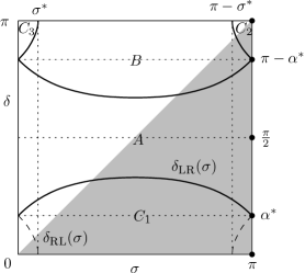
(a) Subdivision of $\Gamma$

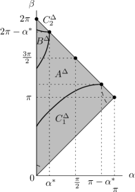
(b) Subdivision of $\Delta$

Figure 12: The subdivision of $\Gamma$ and $\Delta$ for $d=1$

It is clear from this description that the five regions $A$, $B$, $C_{1}$, $C_{2}$, and $C_{3}$ are $\sigma$-monotone, meaning that a line parallel to the $\delta$-axis intersects each region in a single interval. We will also need that the region $B^{\Delta}$ is monotone with respect to the $\alpha$-direction. The proof by elementary calculations is again given in the appendix.

Lemma 7.

For $0<d<2$, there are two continuous functions $\alpha\mapsto\beta_{\text{\tiny RL}}(\alpha)$ and $\alpha\mapsto\beta_{\text{\tiny LR}}(\alpha)$ defined on the interval $[0,\alpha^{\ast}]$ such that $\beta_{\text{\tiny LR}}(\alpha^{\ast})=\beta_{\text{\tiny RL}}(\alpha^{\ast})=2\pi-\alpha^{\ast}$, and such that for $0\leqslant\alpha<\alpha^{\ast}$ we have

• $\alpha+\pi<\beta_{\text{\tiny RL}}(\alpha)<2\pi-\alpha^{\ast}<\beta_{\text{\tiny LR}}(\alpha)<2\pi-\alpha$;

• $d_{\text{\tiny RL}}<2$ for $\beta<\beta_{\text{\tiny RL}}(\alpha)$, $d_{\text{\tiny RL}}=2$ for $\beta=\beta_{\text{\tiny RL}}(\alpha)$, and $d_{\text{\tiny RL}}>2$ for $\beta>\beta_{\text{\tiny RL}}(\alpha)$;

• $d_{\text{\tiny LR}}<2$ for $\beta<\beta_{\text{\tiny LR}}(\alpha)$, $d_{\text{\tiny LR}}=2$ for $\beta=\beta_{\text{\tiny LR}}(\alpha)$, and $d_{\text{\tiny LR}}>2$ for $\beta>\beta_{\text{\tiny LR}}(\alpha)$;

The function $\beta_{\text{\tiny LR}}$ is a monotonically decreasing function of $\alpha$, and we have

$$B^{\Delta}=\big{\{}(\alpha,\beta)\mathrel{\big{|}}\alpha\in[0,\alpha^{\ast}),\;\beta_{\text{\tiny RL}}(\alpha)\leqslant\beta<\beta_{\text{\tiny LR}}(\alpha)\big{\}}.$$

6 Explicit expressions for the length of $\mathit{LRL}$- and $\mathit{RLR}$-paths

In this section we develop explicit formulas for the length of $\mathit{LRL}$- and $\mathit{RLR}$-paths.

We start by a change of perspective, and consider all configurations where $d_{\text{\tiny L}}$ is fixed. We choose a coordinate system where the line $\ell_{S}\ell_{F}$ is horizontal, and $\ell_{S}$ lies to the left of $\ell_{F}$, see Figure 13(a).

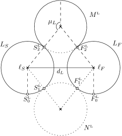
(a) $\mathit{LRL}$-paths

(b) $\mathit{RLR}$-paths

Figure 13: Locations of $S$ and $F$ on their disks

We have drawn the two unit-radius disks $M^{\text{\tiny L}}$ and $N^{\text{\tiny L}}$ tangent to $L_{S}$ and $L_{F}$. The points of tangency are $S^{\text{\tiny L}}_{2}$ and $F^{\text{\tiny L}}_{2}$ for $M^{\text{\tiny L}}$, and $S^{\text{\tiny L}}_{1}$ and $F^{\text{\tiny L}}_{1}$ for $N^{\text{\tiny L}}$. Dubins [11] showed that the length of the middle circular arc of a $\mathit{CCC}$-path is larger than $\pi$, and so it lies on $M^{\text{\tiny L}}$.

So any $\mathit{LRL}$-path first follows a leftwards arc on $L_{S}$, then switches to $M^{\text{\tiny L}}$ at $S^{\text{\tiny L}}_{2}$, follows the rightwards arc on $M^{\text{\tiny L}}$ until it reaches $F^{\text{\tiny L}}_{2}$, and finally follows a leftwards arc on $L_{F}$. We note that the middle arc on $M^{\text{\tiny L}}$ does not depend on the specific endpoints $S$ and $F$, it is determined entirely by $S^{\text{\tiny L}}_{2}$ and $F^{\text{\tiny L}}_{2}$, and therefore by $d_{\text{\tiny L}}$. Let $\mu_{\text{\tiny L}}$ denote half the length of the middle circular arc $\ddddot{S^{\text{\tiny L}}_{2}F^{\text{\tiny L}}_{2}}$. We have $\pi/2<\mu_{\text{\tiny L}}\leqslant\pi$, and $4\sin(\pi-\mu_{\text{\tiny L}})=d_{\text{\tiny L}}$, so that we have

$$\mu_{\text{\tiny L}} =\pi-4\arcsin({d_{\text{\tiny L}}}/{4}).$$

The same considerations apply to $\mathit{RLR}$-paths, see Figure 13(b). We define $\mu_{\text{\tiny R}}$ as half the length of the middle circular arc of the $\mathit{RLR}$-path, and obtain

$$\mu_{\text{\tiny R}} =\pi-4\arcsin({d_{\text{\tiny R}}}/{4}).$$

It is easy to express the length of $\mathit{CCC}$-paths up to a multiple of $2\pi$:

Lemma 8.

For any $\sigma,\delta$, we have

$$\operatorname{\textsc{lrl}}(\sigma,\delta) \equiv 4\mu_{\text{\tiny L}}+2\delta\pmod{2\pi},$$

$$\operatorname{\textsc{rlr}}(\sigma,\delta) \equiv 4\mu_{\text{\tiny R}}-2\delta\pmod{2\pi}.$$

Proof.

An $\mathit{LRL}$-path consists of an initial left-turning arc of length $\gamma_{1}$ on $L_{S}$, a right-turning arc of length $2\mu_{\text{\tiny L}}$ on the middle disk, and a final left-turning arc of length $\gamma_{2}$ on $L_{F}$. This means that the total change in orientation is $\gamma_{1}-2\mu_{\text{\tiny L}}+\gamma_{2}$. On the other hand, since the initial orientation is $\alpha$ and the final orientation is $\beta$, this must be equal, up to multiples of $2\pi$, to $\beta-\alpha=2\delta$. It follows that

$$\operatorname{\textsc{lrl}}=\gamma_{1}+\gamma_{2}+2\mu_{\text{\tiny L}}=\gamma_{1}-2\mu_{\text{\tiny L}}+\gamma_{2}+4\mu_{\text{\tiny L}}\equiv 2\delta+4\mu_{\text{\tiny L}}\pmod{2\pi}.$$

For $\mathit{RLR}$-paths, we can similarly observe that $-\gamma_{1}+2\mu_{\text{\tiny R}}-\gamma_{2}\equiv 2\delta\pmod{2\pi}$ (here, $\gamma_{1}$ and $\gamma_{2}$ are the right-turning arcs) and obtain

$$\operatorname{\textsc{rlr}}=\gamma_{1}+\gamma_{2}+2\mu_{\text{\tiny R}}=4\mu_{\text{\tiny R}}-(-\gamma_{1}+2\mu_{\text{\tiny R}}-\gamma_{2})\equiv 4\mu_{\text{\tiny R}}-2\delta\pmod{2\pi}.\qed$$

Lemma 8 expresses the length of $\mathit{CCC}$-paths only up to a multiple of $2\pi$. Indeed, when considering the length as a function of the endpoints $S$ and $F$ on the fixed disks $L_{S}$ and $L_{F}$, then the length jumps by $2\pi$ when $S$ crosses $S_{2}^{\textsc{l}}$, or when $F$ crosses $F_{2}^{\textsc{l}}$ (see Figure 13(a)), even though $\mu_{\text{\tiny L}}$ is constant and $\delta$ changes continuously. It is therefore important to understand the possible locations of the endpoints $S$ and $F$ along the disks $L_{S}$ and $L_{F}$:

Lemma 9.

We have

• $S$ lies on the counter-clockwise arc $\ddddot{S^{\text{\tiny L}}_{1}S^{\text{\tiny L}}_{2}}$ of $L_{S}$ if and only if $d_{\text{\tiny RL}}<2$;

• $F$ lies on the clockwise arc $\ddddot{F^{\text{\tiny R}}_{2}F^{\text{\tiny R}}_{1}}$ of $R_{F}$ if and only if $d_{\text{\tiny RL}}<2$;

• $S$ lies on the clockwise arc $\ddddot{S^{\text{\tiny R}}_{1}S^{\text{\tiny R}}_{2}}$ of $R_{S}$ if and only if $d_{\text{\tiny LR}}<2$;

• $F$ lies on the counter-clockwise arc $\ddddot{F^{\text{\tiny L}}_{2}F^{\text{\tiny L}}_{1}}$ of $L_{F}$ if and only if $d_{\text{\tiny LR}}<2$.

If $d_{\text{\tiny RL}}\geqslant 2$ and in addition $0\leqslant\alpha\leqslant\pi/2$, then $S$ lies on the counter-clockwise arc $\ddddot{S^{\text{\tiny L}}_{0}S^{\text{\tiny L}}_{1}}$ of $L_{S}$.

Proof.

Consider the position of $R_{S}$ as $S$ moves once around the fixed circle $L_{S}$. The center $r_{S}$ describes a circle of radius two around $\ell_{S}$. When $S=S^{\text{\tiny L}}_{1}$, we have $R_{S}=N^{\text{\tiny L}}$, when $S=S^{\text{\tiny L}}_{2}$, we have $R_{S}=M^{\text{\tiny L}}$. If $d_{\text{\tiny RL}}<2$, we have $R_{S}\cap L_{F}\neq\emptyset$, and so $S$ must lie on the counter-clockwise arc $\ddddot{S^{\text{\tiny L}}_{1}S^{\text{\tiny L}}_{2}}$. If $d_{\text{\tiny RL}}\geqslant 2$, we have $R_{S}\cap L_{F}=\emptyset$, and $S$ must lie on the complementary arc $\ddddot{S^{\text{\tiny L}}_{2}S^{\text{\tiny L}}_{1}}$. The same argument applies to $\mathit{RLR}$-paths to determine the location of $F$. We argue similarly for $d_{\text{\tiny LR}}<2$ and $d_{\text{\tiny LR}}\geqslant 2$.

We observe next that the starting orientation at $S$, which is the forward tangent to $L_{S}$ at $S$, and the vector $\overrightarrow{SF}$ must make an angle of $\alpha$. Since $F\in L_{F}$, this is impossible for $0\leqslant\alpha\leqslant\pi/2$ and $S$ on the long counter-clockwise arc $\ddddot{S^{\text{\tiny L}}_{2}S^{\text{\tiny L}}_{0}}$, and so $d_{\text{\tiny RL}}\geqslant 2$ with $0\leqslant\alpha\leqslant\pi/2$ implies that $S\in\ddddot{S^{\text{\tiny L}}_{0}S^{\text{\tiny L}}_{1}}$. ∎

Given the location of the endpoints on the disks $L_{S}$ and $L_{F}$, we can strengthen Lemma 8 by computing the exact multiple of $2\pi$ that appears in the length. The proof, based on bounding the possible lengths of $\gamma_{1}$ and $\gamma_{2}$, the initial arc and the final arc of a $\mathit{CCC}$-path, is given in the appendix.

Lemma 10.

We have

• For $(\sigma,\delta)\in A$, $\operatorname{\textsc{lrl}}(\sigma,\delta)=4\mu_{\text{\tiny L}}+2\delta-2\pi$ and $\operatorname{\textsc{rlr}}(\sigma,\delta)=4\mu_{\text{\tiny R}}-2\delta$;

• For $(\sigma,\delta)\in B$, $\operatorname{\textsc{lrl}}(\sigma,\delta)=4\mu_{\text{\tiny L}}+2\delta-2\pi$ and $\operatorname{\textsc{rlr}}(\sigma,\delta)=4\mu_{\text{\tiny R}}-2\delta+2\pi$.

Understanding the position of the endpoints also allows us to extend Lemma 1 to include the $\mathit{LRL}$-path, at least when the original configuration is in case $B^{\Delta}$. We need this to prove that $\operatorname{dub}(d)=2\pi$ for all $d\geqslant 2$ by simply appealing to monotonicity.

Lemma 11.

Let $d_{1}<d_{2}$, and $(\alpha,\beta)\in B^{\Delta}$ (where $B^{\Delta}$ is defined for $d_{1}$). If there is an $\mathit{LRL}$-path of length $\ell$ from $(0,0,\alpha)$ to $(d_{1},0,\beta)$, then there is a path of length $\ell+(d_{2}-d_{1})$ from $(0,0,\alpha)$ to $(d_{2},0,\beta)$.

Proof.

We only have to prove that the $\mathit{LRL}$-path has a horizontal tangent oriented in the positive $x$-direction. Assume this is not the case, so there is no point on the path were the orientation is $0$ or $2\pi$. The path starts at orientation $\alpha$, the orientation increases to $\alpha+\gamma_{1}$, decreases to $\alpha+\gamma_{1}-2\mu_{\text{\tiny L}}$, and increases again to $\beta=\alpha+\gamma_{1}-2\mu_{\text{\tiny L}}+\gamma_{2}$, without ever leaving the open range $(0,2\pi)$. But by Lemma 3, $(\alpha,\beta)\in B^{\Delta}$ implies $d_{\text{\tiny RL}}\geqslant 2$ and $0\leqslant\alpha\leqslant\pi/2$ and thus, by Lemma 9 the point $S$ lies on the counter-clockwise arc $\ddddot{S^{\text{\tiny L}}_{0}S^{\text{\tiny L}}_{1}}$ of $L_{S}$. Since $\angle S^{\text{\tiny L}}_{0}\ell_{S}S^{\text{\tiny L}}_{2}=\mu_{\text{\tiny L}}$ and $\angle S^{\text{\tiny L}}_{1}\ell_{S}S^{\text{\tiny L}}_{2}=2\pi-\mu_{\text{\tiny L}}$, we have $2\mu_{\text{\tiny L}}-\pi\leqslant\gamma_{1}\leqslant\mu_{\text{\tiny L}}$ and $0\leqslant\gamma_{2}\leqslant 2\mu_{\text{\tiny L}}-\pi$. This implies that $\gamma_{1}+\gamma_{2}\leqslant 2\mu_{\text{\tiny L}}$, and so $\beta\leqslant\alpha$, a contradiction to $(\alpha,\beta)\in B^{\Delta}$. ∎

The explicit expressions for the $\mathit{LRL}$-path length in Lemma 10 allow us to study its derivative, and to show that the length of $\mathit{LRL}$-paths is monotone in $\alpha$ and $\beta$, at least for the cases of interest to us. The calculations involving these derivatives are given in the appendix.

Lemma 12.

We have

• For $(\alpha,\beta)\in A^{\Delta}$, the function $\beta\mapsto\operatorname{\textsc{lrl}}(\alpha,\beta)$ is increasing;

• For $(\alpha,\beta)\in B^{\Delta}$, the function $\alpha\mapsto\operatorname{\textsc{lrl}}(\alpha,\beta)$ is decreasing, while $\beta\mapsto\operatorname{\textsc{lrl}}(\alpha,\beta)$ is increasing; Moreover, if $(\alpha,\beta)\in B^{\Delta}$ and $\beta\geqslant{3\pi}/{2}$, then $\frac{\partial\operatorname{\textsc{lrl}}}{\partial\beta}(\alpha,\beta)\geqslant 1$.

7 Case A

When $d<2$, both $\mathit{LRL}$- and $\mathit{RLR}$-paths exist for any $(\sigma,\delta)\in\Gamma$. We define three functions l, r, and c on $\Gamma$:

$$\textsc{l}(\sigma,\delta) =4\mu_{\text{\tiny L}}(\sigma,\delta)+2\delta-2\pi$$ (11)

$$\textsc{r}(\sigma,\delta) =4\mu_{\text{\tiny R}}(\sigma,\delta)-2\delta$$ (12)

$$\textsc{c}(\sigma,\delta) =\min\{\textsc{l}(\sigma,\delta),\textsc{r}(\sigma,\delta)\}.$$ (13)

While these functions are defined and continuous everywhere on $\Gamma$, we have shown in Lemma 10 only that $\operatorname{\textsc{lrl}}(\sigma,\delta)=\textsc{l}(\sigma,\delta)$ for $(\sigma,\delta)\in A\cup B$, and $\operatorname{\textsc{rlr}}(\sigma,\delta)=\textsc{r}(\sigma,\delta)$ for $(\sigma,\delta)\in A$.

Recall that $\alpha^{\ast}=\arcsin({d}/{2})$. We define the following rectangle $\Xi\subset\Gamma$:

$$\Xi:\quad 0\leqslant\sigma\leqslant\pi\quad\text{and}\quad\alpha^{\ast}\leqslant\delta\leqslant\pi-\alpha^{\ast}.$$

Note that $A\subset\Xi$ (see Figure 12(a)). It will be easier to work with the rectangular domain $\Xi$ rather than the curved region $A$, as long as we keep in mind that $\textsc{c}(\sigma,\delta)$ is the length of the shortest $\mathit{CCC}$-path for $(\sigma,\delta)\in A$ only.

By studying the derivatives of the functions $\textsc{l}(\sigma,\delta)$ and $\textsc{r}(\sigma,\delta)$, we can show that they are monotone in $\sigma$- and $\delta$-direction. The calculations are given in the appendix.

Lemma 13.

For $(\sigma,\delta)\in\Xi$, the function

• $\sigma\mapsto\textsc{l}(\sigma,\delta)$ is decreasing, while $\sigma\mapsto\textsc{r}(\sigma,\delta)$ is increasing,

• $\delta\mapsto\textsc{l}(\sigma,\delta)$ is increasing, while $\delta\mapsto\textsc{r}(\sigma,\delta)$ is decreasing.

Monotonicity of l and r implies that neither has a local extremum in the interior of $\Xi$, and a local extremum can only occur on the set $\Lambda$ of points $(\sigma,\delta)$ with $\textsc{l}(\sigma,\delta)=\textsc{r}(\sigma,\delta)$ (see Figure 14).

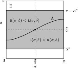
Figure 14: The curve $\Lambda$ where $\textsc{l}(\sigma,\delta)=\textsc{r}(\sigma,\delta)$ in rectangle $\Xi$ (shaded region), shown for $d=1$.

In the appendix we use Lagrange multipliers to prove that in fact the only local extremum is at $(\pi/2,\pi/2)$.

Lemma 14.

The function $\textsc{c}(\sigma,\delta)$ has no local extremum in the interior of $\Xi$ except at $(\pi/2,\pi/2)$.

Since $\textsc{c}(\sigma,\delta)$ is continuous, it assumes its maximum on $\Xi$. By Lemma 14, this must happen either at $(\sigma,\delta)=(\pi/2,\pi/2)$, or on the boundary of $\Xi$, at a point $(\sigma_{\text{\tiny A}},\delta_{\text{\tiny A}})$ where $\textsc{l}(\sigma_{\text{\tiny A}},\delta_{\text{\tiny A}})=\textsc{r}(\sigma_{\text{\tiny A}},\delta_{\text{\tiny A}})$. This must happen either on the vertical side $\sigma=\pi,\pi/2<\delta\leqslant\pi-\alpha^{\ast}$, or on the horizontal side $\delta=\pi-\alpha^{\ast},\pi/2<\sigma\leqslant\pi$. The point $(\sigma_{\text{\tiny A}},\delta_{\text{\tiny A}})$ is unique if we require $\sigma_{\text{\tiny A}}+\delta_{\text{\tiny A}}>\pi$, and there is a symmetric point $(\pi-\sigma_{\text{\tiny A}},\pi-\delta_{\text{\tiny A}})$. Let us define the function $\textsc{a}(d)$ for $0\leqslant d<2$ as

$$\textsc{a}(d) =\operatorname{\textsc{lrl}}(\sigma_{\text{\tiny A}},\delta_{\text{\tiny A}})=\operatorname{\textsc{rlr}}(\sigma_{\text{\tiny A}},\delta_{\text{\tiny A}}).$$ (14)

There is an important breakpoint at $d=\sqrt{2}$:

Lemma 15.

The maximum $\textsc{a}(d)$ occurs with $\sigma_{\text{\tiny A}}=\pi$ when $0\leqslant d\leqslant\sqrt{2}$, and with $\delta_{\text{\tiny A}}=\pi-\alpha^{\ast}$ when $\sqrt{2}\leqslant d<2$.

Proof.

We evaluate $\textsc{l}(\pi,\pi-\alpha^{\ast})$ and $\textsc{r}(\pi,\pi-\alpha^{\ast})$. Using (6) and (7), we have

$$d_{\text{\tiny L}}(\pi,\pi-\alpha^{\ast}) =2d$$

$$d_{\text{\tiny R}}(\pi,\pi-\alpha^{\ast}) =0,$$

which implies by (11) and (12):

$$\textsc{l}(\pi,\pi-\alpha^{\ast}) =4\pi-6\alpha^{\ast},$$

$$\textsc{r}(\pi,\pi-\alpha^{\ast}) =2\pi+2\alpha^{\ast}.$$

Since $\alpha^{\ast}=\arcsin(d/2)$, we have $\textsc{r}(\pi,\pi-\alpha^{\ast})<\textsc{l}(\pi,\pi-\alpha^{\ast})$ for $d<\sqrt{2}$, equality for $d=\sqrt{2}$, and $\textsc{r}(\pi,\pi-\alpha^{\ast})>\textsc{l}(\pi,\pi-\alpha^{\ast})$ for $d>\sqrt{2}$. In the first case, Lemma 13 implies that the maximum must occur on the vertical side at $\sigma=\pi$, in the last case it must occur on the horizontal side at $\delta=\pi-\alpha^{\ast}$. For $d=\sqrt{2}$ the maximum occurs at the corner $(\sigma_{A},\delta_{A})=(\pi,\pi-\alpha^{\ast})$. ∎

Again using Lagrange multipliers, we prove in the appendix that the functions $d\mapsto\textsc{a}(d)$ and $d\mapsto\textsc{a}(d)-d$ are monotone.

Lemma 16.

On the interval $0\leqslant d\leqslant\sqrt{2}$, the function

• $d\mapsto\textsc{a}(d)$ is monotonically increasing,

• $d\mapsto\textsc{a}(d)-d$ is monotonically decreasing.

It remains to decide whether $\textsc{c}(d,\pi/2,\pi/2)$ or $\textsc{a}(d)$ is larger.

Lemma 17.

For $0<d\leqslant\sqrt{2}$, we have $\max_{(\sigma,\delta)\in\Xi}\textsc{c}(d,\sigma,\delta)=\textsc{a}(d)$.

Proof.

For $0\leqslant d\leqslant\sqrt{2}$ and $(\sigma,\delta)=(\pi/2,\pi/2)$, we have

$$d_{\text{\tiny L}}^{2} =d^{2}+4\quad\text{by~{}(\ref{eq:dl-sigma-delta})}$$

$$\mu_{\text{\tiny L}} =\pi-\arcsin(\sqrt{d^{2}+4}/4)$$

$$\textsc{l}(d,\pi/2,\pi/2) =4\mu_{\text{\tiny L}}+2\delta-2\pi=3\pi-4\arcsin(\sqrt{d^{2}+4}/4).$$

Since $\arcsin$ is an increasing function, $d\mapsto\textsc{l}(d,\pi/2,\pi/2)$ is a decreasing function. We therefore have

$$\textsc{l}(d,\pi/2,\pi/2)<\textsc{l}(0,\pi/2,\pi/2)=7\pi/3.$$

On the other hand, by Lemma 16, the function $d\mapsto\textsc{a}(d)$ is increasing, and so $\textsc{a}(d)\geqslant\textsc{a}(0)=7\pi/3>\textsc{l}(d,\pi/2,\pi/2)$. ∎

We now justify that it suffices to study $\mathit{CCC}$-paths in case A, as no other path type can be shorter. Since $\mathit{LSR}$- and $\mathit{RSL}$-paths do not exist, it is enough to show the following lemma:

Lemma 18.

For $(\sigma,\delta)\in A$, we have

$$\operatorname{\textsc{lrl}}(\sigma,\delta) \leqslant\operatorname{\textsc{lsl}}(\sigma,\delta)$$

$$\operatorname{\textsc{rlr}}(\sigma,\delta) \leqslant\operatorname{\textsc{rsr}}(\sigma,\delta).$$

Proof.

Let $\gamma_{1}$ and $\gamma_{2}$ be the length of the left-turning arcs of an $\mathit{LRL}$-path. By Lemma 9, the endpoints $S$ and $F$ lie on the counterclockwise arcs $\ddddot{S^{\text{\tiny L}}_{1}S^{\text{\tiny L}}_{2}}$ of $L_{S}$ and $\ddddot{F^{\text{\tiny L}}_{2}F^{\text{\tiny L}}_{1}}$ of $L_{F}$ (see Figure 13(a)).

On the other hand, the $\mathit{LSL}$-path turns left on $L_{S}$ until $S^{\text{\tiny L}}_{0}$, goes along the tangent to $F^{\text{\tiny L}}_{0}$, then turns left on $L_{F}$ until it reaches $F$. Since $\angle S^{\text{\tiny L}}_{2}\ell_{S}S^{\text{\tiny L}}_{0}=\mu_{\text{\tiny L}}$ and $|S^{\text{\tiny L}}_{0}F^{\text{\tiny L}}_{0}|=d_{\text{\tiny L}}$, we have

$$\operatorname{\textsc{lsl}}-\operatorname{\textsc{lrl}} =d_{\text{\tiny L}}+2(2\pi-\mu_{\text{\tiny L}})-2\mu_{\text{\tiny L}}=d_{\text{\tiny L}}+4(\pi-\mu_{\text{\tiny L}})\geqslant 0$$

since $\mu_{\text{\tiny L}}\leqslant\pi$. The analogous argument shows that $\operatorname{\textsc{rlr}}\leqslant\operatorname{\textsc{rsr}}$. ∎

Putting everything together, the following two lemmas describe $\operatorname{dub}_{A}(d)$.

Lemma 19.

For $0<d<\sqrt{2}$, $\operatorname{dub}_{A}(d)=\textsc{a}(d)-d$. In other words, the maximum is realized by the unique point $(\sigma_{\text{\tiny A}},\delta_{\text{\tiny A}})$ on the segment $\sigma=\pi$, $\pi/2\leqslant\delta\leqslant\pi-\alpha^{\ast}$ where $\textsc{l}(d,\sigma_{\text{\tiny A}},\delta_{\text{\tiny A}})=\textsc{r}(d,\sigma_{\text{\tiny A}},\delta_{\text{\tiny A}})$. We have $\textsc{a}(d)>2\pi+2\alpha^{\ast}$.

Proof.

By Lemma 17, we have $\max_{(\sigma,\delta)\in\Xi}\textsc{c}(d,\sigma,\delta)=\textsc{a}(d)$, and the maximum is assumed at the point $(\sigma_{\text{\tiny A}},\delta_{\text{\tiny A}})\in A^{\Delta}$. By Lemma 18, we have $\ell(d,\sigma,\delta)=\textsc{c}(d,\sigma,\delta)$ for $(\sigma,\delta)\in A^{\Delta}$. Since $(\sigma_{\text{\tiny A}},\delta_{\text{\tiny A}})\in A^{\Delta}\subset\Xi$, this means that $\operatorname{dub}_{A}(d)=\sup_{(\sigma,\delta)\in A^{\Delta}}\ell(d,\sigma,\delta)-d=\textsc{c}(d,\sigma_{\text{\tiny A}},\delta_{\text{\tiny A}})-d=\textsc{a}(d)-d$. Finally, the last inequality follows from $\textsc{a}(d)>\textsc{c}(\pi,\pi-\alpha^{\ast})=\textsc{r}(\pi,\pi-\alpha^{\ast})=2\pi+2\alpha^{\ast}$, as we observed in the proof of Lemma 15. ∎

Lemma 20.

For $\sqrt{2}\leqslant d<2$, we have $\operatorname{dub}_{A}(d)\leqslant\max\{2\pi,\operatorname{dub}_{B}(d)\}$.

Proof.

Let $\bar{A}$ be the closure of $A^{\Delta}$. Since $\bar{A}$ is compact and c is continuous, there is a point $(\sigma,\delta)\in\bar{A}$ where $\textsc{c}(\sigma,\delta)$ assumes its maximum. By Lemma 14 this is necessarily a point where $\textsc{l}(\sigma,\delta)=\textsc{r}(\sigma,\delta)$, and either $(\sigma,\delta)=(\pi/2,\pi/2)$, or $(\sigma,\delta)$ lies on the boundary of $\bar{A}$. By Lemma 15, it cannot occur on the vertical side of $\Xi$.

Assume first that $\delta<\pi/2$. By Lemma 13, we must then have $\sigma<\pi/2$. Using Lemmas 13 and 12, we have

$$\textsc{c}(d,\sigma,\delta) \leqslant\textsc{l}(d,\sigma,\delta)\leqslant\textsc{l}(d,\delta,\delta)\leqslant\textsc{l}(d,\pi/2,\pi/2).$$

We observed in the proof of Lemma 17 that $\textsc{l}(d,\pi/2,\pi/2)$ is a decreasing function of $d$. For $d=\sqrt{2}$, we already have $\textsc{l}(\sqrt{2},\pi/2,\pi/2)=3\pi-4\arcsin(\sqrt{6}/4)<2\pi+\sqrt{2}$, and so $\textsc{c}(d,\sigma,\delta)\leqslant d+2\pi$. The same argument covers the case where $(\sigma,\delta)=(\pi/2,\pi/2)$.

It remains to consider the possibility that $\delta>\pi/2$. In this case $(\sigma,\delta)$ lies on the common boundary of $A^{\Delta}$ and $B^{\Delta}$. On this boundary we have $d_{\text{\tiny RL}}=2$, so $R_{S}$ and $L_{F}$ touch. Note that in this case $(\sigma,\delta)$ lies in $B^{\Delta}$, not in $A^{\Delta}$. It remains to observe that then the $\mathit{RLR}$-path is identical to the $\mathit{RSL}$-path, so we have $\operatorname{\textsc{rsl}}(\sigma,\delta)=\operatorname{\textsc{lrl}}(\sigma,\delta)$. We will prove in Lemma 22 that in $B^{\Delta}$ these two path types are always shortest, and so $\textsc{c}(d,\sigma,\delta)\leqslant\operatorname{dub}_{B}(d)+d$. ∎

8 Case B

It was proven by Goaoc et al. [13] that for any $\mathit{CSC}$-path type (that is, one of the types $\mathit{LSR}$, $\mathit{RSL}$, $\mathit{LSL}$, or $\mathit{RSR}$), the length of a path of this type from $(0,0,\alpha)$ to $(d,0,\beta)$ is differentiable at any point $(\alpha,\beta)\in\square$ where such a path exists and both its circular arcs have non-zero length. For the case of $\mathit{RSL}$-paths, they prove specifically that

$$\frac{\partial}{\partial\alpha}\operatorname{\textsc{rsl}}(\alpha,\beta) =1-\cos\gamma_{\text{\tiny R}}$$ (15)

$$\frac{\partial}{\partial\beta}\operatorname{\textsc{rsl}}(\alpha,\beta) =1-\cos\gamma_{\text{\tiny L}},$$ (16)

where $\gamma_{\text{\tiny R}}$ and $\gamma_{\text{\tiny L}}$ are the lengths of the right-turning and the left-turning circular arc on the path.

We recall that case B is the situation where $d_{\text{\tiny LR}}(\alpha,\beta)<2$ and $d_{\text{\tiny RL}}(\alpha,\beta)\geqslant 2$. For $0<d<2$, Lemma 7 gives an explicit description of the region $B^{\Delta}$, using the two functions $\beta_{\text{\tiny RL}}(\alpha)$ and $\beta_{\text{\tiny LR}}(\alpha)$. Let us define two extended regions:

$$B^{\circ} =\big{\{}(\alpha,\beta)\mathrel{\big{|}}0\leqslant\alpha\leqslant\alpha^{\ast},\;\beta_{\text{\tiny RL}}(\alpha)\leqslant\beta\leqslant 2\pi-\alpha\big{\}},$$

$$\bar{B} =\big{\{}(\alpha,\beta)\mathrel{\big{|}}0\leqslant\alpha\leqslant\alpha^{\ast},\;\beta_{\text{\tiny RL}}(\alpha)\leqslant\beta\leqslant\beta_{\text{\tiny LR}}(\alpha)\big{\}}.$$

So $\bar{B}$ is the closure of $B^{\Delta}$, while $B^{\circ}$ is the union $B^{\Delta}\cup C^{\Delta}_{2}$ (see Figure 12(b)).

We now investigate where the three segments of an $\mathit{RSL}$-path can vanish in $B^{\circ}$: First, the $S$-segment vanishes exactly if $d_{\text{\tiny RL}}=2$. This happens exactly on the lower boundary of $B^{\circ}$. By Lemma 9, $S$ lies on the arc $\ddddot{S^{\text{\tiny L}}_{0}S^{\text{\tiny L}}_{1}}$ of $L_{S}$ (see Figure 13), and so $0\leqslant\gamma_{\text{\tiny R}}\leqslant 2\alpha^{\ast}$. If $\gamma_{\text{\tiny R}}=0$, then we must have $S=S^{\text{\tiny L}}_{0}$ and therefore $F=F^{\text{\tiny L}}_{0}$. This is the case $(\alpha,\beta)=(0,2\pi)$. Finally, if $\gamma_{\text{\tiny L}}=0$, then $F$ must lie on the arc $\ddddot{F^{\text{\tiny L}}_{1}F^{\text{\tiny L}}_{0}}$, and we have $2\pi-\beta\leqslant\alpha$ (see Figure 15). Equality holds only for $S=S^{\text{\tiny L}}_{1}$, $F=F^{\text{\tiny L}}_{1}$, which is the case $(\alpha,\beta)=(\alpha^{\ast},2\pi-\alpha^{\ast})$. In all other cases, $2\pi-\beta<\alpha$ is a contradiction to $(\alpha,\beta)\in\Delta$.

Figure 15: When $\gamma_{\text{\tiny L}}$ vanishes.

The above implies that $\operatorname{\textsc{rsl}}(\alpha,\beta)$ is differentiable in any point in the interior of $B^{\circ}$. The function is continuous everywhere except at the two points $(\alpha,\beta)=(0,2\pi)$ and $(\alpha,\beta)=(\alpha^{\ast},2\pi-\alpha^{\ast})$. At the first point, the $\mathit{RSL}$-path degenerates to the line segment $\overline{SF}$ of length $d$, while the limit of $\operatorname{\textsc{rsl}}(\alpha,\beta)$ for $(\alpha,\beta)\rightarrow(0,2\pi)$ is $d+2\pi$. For the second point $(\alpha^{\ast},2\pi-\alpha^{\ast})$, consider Figure 11(a). At this point, both the straight segment and the left-turning arc vanish at the same time, and the length of the path is only $|\ddddot{SF}|=2\alpha^{\ast}$. However, for $(\alpha,\beta)\rightarrow(\alpha^{\ast},2\pi-\alpha^{\ast})$, the limit of $\operatorname{\textsc{rsl}}(\alpha,\beta)$ is $|\ddddot{SF}|+2\pi=2\alpha^{\ast}+2\pi$. We observe that this is exactly the value of $\operatorname{\textsc{rlr}}(\alpha^{\ast},2\pi-\alpha^{\ast})$, as the final right-turning arc of the $\mathit{RLR}$-path vanishes.

We therefore define the following function on $B^{\circ}$:

$$\operatorname{\textsc{rsl}^{\ast}}(\alpha,\beta) =\begin{cases}d+2\pi&\text{for $(\alpha,\beta)=(0,2\pi)$}\\ 2\alpha^{\ast}+2\pi&\text{for $(\alpha,\beta)=(\alpha^{\ast},2\pi-\alpha^{\ast})$}\\ \operatorname{\textsc{rsl}}(\alpha,\beta)&\text{else}\end{cases}$$

Overview.

The main goal of this section is to show that for $\sqrt{2}\leqslant d<2$, $\operatorname{dub}_{B}(d)$ is determined by a unique point $(\alpha_{B},\beta_{B})$ on the curve $\beta_{\text{\tiny LR}}$ such that $\operatorname{\textsc{rsl}^{\ast}}(\alpha_{B},\beta_{B})=\operatorname{\textsc{lrl}}(\alpha_{B},\beta_{B})$. To prove this, we first show that the function $\beta\mapsto\operatorname{\textsc{rsl}^{\ast}}(\alpha,\beta)$ is increasing (Lemma 21). Since the function $\beta\mapsto\operatorname{\textsc{lsl}}(\alpha,\beta)$ is increasing in $B^{\Delta}$ as well (Lemma 12), the function $\min\{\operatorname{\textsc{rsl}^{\ast}}(\alpha,\beta),\operatorname{\textsc{lrl}}(\alpha,\beta)\}$ must assume its maximum on the curve $\beta_{\text{\tiny LR}}$ in $\bar{B}$.

Lemma 22 shows that $\operatorname{dub}_{B}(d)$ is indeed determined by the $\mathit{RSL}$-path and the $\mathit{LRL}$-path only. Finally, we will prove that the function $d\mapsto\operatorname{dub}_{B}(d)$ is monotonically decreasing.

We start by studying the derivatives of $\operatorname{\textsc{rsl}^{\ast}}(\alpha,\beta)$ to show monotonicity. The short calculations are in the appendix.

Lemma 21.

For $(\alpha,\beta)\in B^{\circ}$, the function

• $\alpha\mapsto\operatorname{\textsc{rsl}^{\ast}}(\alpha,\beta)$ is increasing,

• $\beta\mapsto\operatorname{\textsc{rsl}^{\ast}}(\alpha,\beta)$ is increasing,

• $\alpha\mapsto\operatorname{\textsc{rsl}^{\ast}}(\alpha,2\pi-\alpha)$ is increasing,

• $\operatorname{\textsc{rsl}^{\ast}}(\alpha,\beta)\leqslant\operatorname{\textsc{rsl}^{\ast}}(\alpha^{\ast},2\pi-\alpha^{\ast})=2\alpha^{\ast}+2\pi$.

Let us define the following function $\textsc{b}(d,\alpha,\beta)$ on $B^{\circ}$:

$$\textsc{b}(d,\alpha,\beta) =\min\{\operatorname{\textsc{rsl}^{\ast}}(d,\alpha,\beta),\,\operatorname{\textsc{lrl}}(d,\alpha,\beta)\}.$$ (17)

Our goal will be to determine $\textsc{b}(d)=\sup_{(\alpha,\beta)\in B^{\Delta}}\textsc{b}(d,\alpha,\beta)$, and then to show that $\operatorname{dub}_{B}(d)=\textsc{b}(d)-d$. Since $\textsc{b}(d,\alpha,\beta)$ is continuous, we have $\textsc{b}(d)=\max_{(\alpha,\beta)\in\bar{B}}\textsc{b}(d,\alpha,\beta)$. By Lemmas 12 and 21, we have $\textsc{b}(d,\alpha,\beta)\leqslant\textsc{b}(d,\alpha,\beta_{\text{\tiny LR}}(\alpha))$ for any $(\alpha,\beta)\in\bar{B}$, and so

$$\textsc{b}(d)=\max_{(\alpha,\beta)\in\bar{B}}\textsc{b}(d,\alpha,\beta)=\max_{0\leqslant\alpha\leqslant\alpha^{\ast}}\textsc{b}(d,\alpha,\beta_{\text{\tiny LR}}(\alpha)).$$

We now show that $\operatorname{dub}_{B}(d)=\textsc{b}(d)-d$ by showing that the $\mathit{LRL}$-path or the $\mathit{RSL}$-path is shorter than any other path type. Since there is no $\mathit{LSR}$-path in case B, it suffices to exclude path types $\mathit{LSL}$, $\mathit{RLR}$, and $\mathit{RSR}$. The details can be found in the appendix.

Lemma 22.

For $(\alpha,\beta)\in B^{\Delta}$ we have $\operatorname{\textsc{lsl}}(\alpha,\beta)\geqslant\operatorname{\textsc{lrl}}(\alpha,\beta),$ $\operatorname{\textsc{rlr}}(\alpha,\beta)\geqslant\operatorname{\textsc{lrl}}(\alpha,\beta),$ and $\operatorname{\textsc{rsr}}(\alpha,\beta)\geqslant\operatorname{\textsc{rsl}}(\alpha,\beta)$.

It remains to understand the function $\textsc{b}(d)$. By definition, it is the maximum of the function

$$\alpha\mapsto\textsc{b}(d,\alpha,\beta_{\text{\tiny LR}}(\alpha))=\min\{\operatorname{\textsc{rsl}^{\ast}}(d,\alpha,\beta_{\text{\tiny LR}}(\alpha)),\operatorname{\textsc{lrl}}(d,\alpha,\beta_{\text{\tiny LR}}(\alpha))\},$$

for $0\leqslant\alpha\leqslant\alpha^{\ast}$ for fixed $d$. We first argue that there is a unique $\alpha_{\text{\tiny B}}\in[0,\alpha^{\ast}]$ such that

$$\textsc{b}(d,\alpha,\beta_{\text{\tiny LR}}(\alpha))=\begin{cases}\operatorname{\textsc{rsl}^{\ast}}(d,\alpha,\beta_{\text{\tiny LR}}(\alpha))&\text{ for }\alpha\leqslant\alpha_{\text{\tiny B}}\\ \operatorname{\textsc{lrl}}(d,\alpha,\beta_{\text{\tiny LR}}(\alpha))&\text{ for }\alpha\geqslant\alpha_{\text{\tiny B}}\end{cases}$$

This follows directly from the following lemma, whose proof (based on comparing derivatives) can be found in the appendix.

Lemma 23.

The function $\alpha\mapsto\operatorname{\textsc{lrl}}(\alpha,\beta_{\text{\tiny LR}}(\alpha))-\operatorname{\textsc{rsl}}(\alpha,\beta_{\text{\tiny LR}}(\alpha))$ is monotonically decreasing on $[0,\alpha^{\ast}]$.

By Lemmas 12 and 7, the function $\alpha\mapsto\operatorname{\textsc{lrl}}(d,\alpha,\beta_{\text{\tiny LR}}(\alpha))$ is decreasing. The maximum of $\textsc{b}(d,\alpha,\beta_{\text{\tiny LR}}(\alpha))$ is therefore at $\alpha=0$, at $\alpha=\alpha_{B}$, or is a local maximum of $\operatorname{\textsc{rsl}^{\ast}}(d,\alpha,\beta_{\text{\tiny LR}}(\alpha))$ with $\alpha<\alpha_{B}$.

In the first case $\alpha=0$ a simple geometric argument similar to Lemma 4 shows that $\operatorname{\textsc{rsl}}(d,0,\beta_{\text{\tiny LR}}(0))\leqslant d+2\pi$. Similarly, we show that a local maximum of $\operatorname{\textsc{rsl}^{\ast}}(d,\alpha,\beta_{\text{\tiny LR}}(\alpha))$ implies a path length at most $d+2\pi$. The proof for this technical detail looks at both the path geometry and at the derivatives, and can be found in the appendix.

Lemma 24.

If $\alpha\mapsto\operatorname{\textsc{rsl}^{\ast}}(d,\alpha,\beta_{\text{\tiny LR}}(\alpha))$ has an extremum for $0<\alpha<\alpha^{\ast}$, then $\operatorname{\textsc{rsl}^{\ast}}(d,\alpha,\beta_{\text{\tiny LR}}(\alpha))\leqslant d+2\pi$.

Putting these arguments together, we have shown:

Lemma 25.

For $0<d<2$ if $\operatorname{dub}_{B}(d)>2\pi$, then $\operatorname{dub}_{B}(d)=\textsc{b}(d,\alpha_{\text{\tiny B}},\beta_{\text{\tiny LR}}(\alpha_{\text{\tiny B}}))-d$, where $\alpha_{\text{\tiny B}}$ is the unique value in $[0,\alpha^{\ast}]$ where $\operatorname{\textsc{rsl}^{\ast}}(d,\alpha_{\text{\tiny B}},\beta_{\text{\tiny LR}}(\alpha_{\text{\tiny B}}))=\operatorname{\textsc{lrl}}(d,\alpha_{\text{\tiny B}},\beta_{\text{\tiny LR}}(\alpha_{\text{\tiny B}}))$.

It remains to argue the monotonicity of $d\mapsto\operatorname{dub}_{B}(d)$.

Lemma 26.

For $\sqrt{2}\leqslant d<2$, $\operatorname{dub}_{B}(d)$ decreases monotonically from $\operatorname{dub}_{B}(\sqrt{2})=5\pi/2-\sqrt{2}$ to $\operatorname{dub}_{B}(d^{\ast})=2\pi$ for $d^{\ast}\approx 1.5874$. We have $\operatorname{dub}_{B}(d)\leqslant 2\pi$ for $d\geqslant d^{\ast}$.

Proof.

Assume the function is not monotone, so there is $\sqrt{2}\leqslant d_{1}<d_{4}<2$ such that $2\pi<\operatorname{dub}_{B}(d_{1})<\operatorname{dub}_{B}(d_{4})$. Since $\operatorname{dub}_{B}(d)$ is continuous, it assumes its maximum $D:=\max_{d\in[d_{1},d_{4}]}\operatorname{dub}_{B}(d)$ on the closed interval $[d_{1},d_{4}]$. The set $\{d\in[d_{1},d_{4}]\mid\operatorname{dub}_{B}(d)=D\}$ is compact, and so assumes its infimum, say at $d_{3}$. So we have $\operatorname{dub}_{B}(d_{3})>\operatorname{dub}_{B}(d_{1})>2\pi$, and $\operatorname{dub}_{B}(d)<\operatorname{dub}_{B}(d_{3})$ for $d_{1}\leqslant d<d_{3}$.

By Lemma 25, we have $\operatorname{dub}_{B}(d_{3})=\textsc{b}(d_{3},\alpha_{\text{\tiny B}},\beta_{\text{\tiny B}})-d_{3}$, where $0<\alpha_{\text{\tiny B}}\leqslant\arcsin(d_{3}/2)$ and $\beta_{\text{\tiny B}}=\beta_{\text{\tiny LR}}(\alpha_{\text{\tiny B}})$. Let us define $d_{2}=\max\{d_{1},2\sin(2\pi-\beta_{\text{\tiny B}})\}$. Then $d_{1}\leqslant d_{2}<d_{3}$, and $(\alpha_{\text{\tiny B}},\beta_{\text{\tiny B}})\in B^{\Delta}$ for $d=d_{2}$. Then there is an $\mathit{RSL}$- or $\mathit{LRL}$-path from $(0,0,\alpha_{\text{\tiny B}})$ to $(d_{2},0,\beta_{\text{\tiny B}})$ of length at most $\operatorname{dub}_{B}(d_{2})+d_{2}$. By Lemmas 1 and 11, there is then a path of length $\operatorname{dub}_{B}(d_{2})+d$ from $(0,0,\alpha_{\text{\tiny B}})$ to $(d,0,\beta_{\text{\tiny B}})$ for all $d\geqslant d_{2}$, implying that $\ell(d,\alpha_{\text{\tiny B}},\beta_{\text{\tiny B}})\leqslant\operatorname{dub}_{B}(d_{2})+d$, a contradiction to the assumption that $\operatorname{dub}_{B}(d_{3})>\operatorname{dub}_{B}(d_{2})$.

Continuity and monotonicity of $\operatorname{dub}_{B}(d)$ imply that there must be a value $d^{\ast}$ with $\operatorname{dub}_{B}(d^{\ast})=2\pi$. We have numerically computed the approximation $d^{\ast}\approx 1.5874$. For a given $d$, we first approximate $\alpha_{\text{\tiny B}}$ numerically by binary search on the interval $[0,\alpha^{\ast}]$ using Lemma 23. We can then compute $\beta_{\text{\tiny LR}}(\alpha_{\text{\tiny B}})$ and $\textsc{b}(d)$. ∎

Appendix A Appendix

Proof of Lemma 6

Proof.

We first argue about the curve $\delta_{\text{\tiny LR}}(\sigma)$. From Eq. (8) we have $d_{\text{\tiny LR}}^{2}=d^{2}+4d\cos\delta\sin\sigma+4\cos^{2}\delta$. For $\delta=\alpha^{\ast}$, we have $\cos^{2}\delta=1-\sin^{2}\delta=1-d^{2}/4$, and so $d_{\text{\tiny LR}}^{2}=4+4d\cos\alpha^{\ast}\sin\sigma$. This is equal to $4$ for $\sigma\in\{0,\pi\}$, and otherwise larger than $4$. For $\delta=\pi/2$, we have $d_{\text{\tiny LR}}^{2}=d^{2}<4$. Finally, for $\delta\in(0,\pi/2)$, we have $\frac{\partial}{\partial\delta}d_{\text{\tiny LR}}^{2}=-4d\sin\delta\sin\sigma-8\cos\delta\sin\delta<0$, and so $\delta\mapsto d_{\text{\tiny LR}}$ is a decreasing function for $\sigma\in(0,\pi)$, proving the first claim.

Consider now $d_{\text{\tiny RL}}^{2}=d^{2}-4d\cos\delta\sin\sigma+4\cos^{2}\delta$ by Eq. (9). For $\alpha^{\ast}\leqslant\delta\leqslant\pi/2$, we have $\cos^{2}\delta=1-\sin^{2}\delta\leqslant 1-d^{2}/4$, and so $d_{\text{\tiny RL}}^{2}\leqslant 4$, with equality only for $\sigma\in\{0,\pi\}$ and $\delta=\alpha^{\ast}$ which proves the third claim. On the interval $0\leqslant\sigma\leqslant\sigma^{\ast}$, we have $d_{\text{\tiny RL}}^{2}\geqslant 4$ for $\delta=0$ (with equality only for $\sigma=\sigma^{\ast}$), $d_{\text{\tiny RL}}^{2}\leqslant 4$ for $\delta=\alpha^{\ast}$ (with equality only for $\sigma=0$), and $d_{\text{\tiny RL}}^{2}\geqslant 4$ for $\delta=\pi$. Since for fixed $\sigma$, $d_{\text{\tiny RL}}^{2}=4$ is a quadratic polynomial in $\cos\delta$, it has at most two roots in $0\leqslant\delta\leqslant\pi$, and thus there must be a unique value $0\leqslant\delta_{\text{\tiny RL}}(\sigma)\leqslant\alpha^{\ast}$ on the interval $0\leqslant\sigma\leqslant\sigma^{\ast}$ where $d_{\text{\tiny RL}}=2$. This proves the second claim.

In the remaining region $\sigma^{\ast}<\sigma<\pi-\sigma^{\ast}$, $0\leqslant\delta\leqslant\alpha^{\ast}$, we have $d_{\text{\tiny RL}}^{2}<4$. Indeed, in this region we have $\sin\sigma>d/4$, and so $d_{\text{\tiny RL}}^{2}<D(\sigma,\delta)$, where $D(\sigma,\delta)=d^{2}-d^{2}\cos\delta+4\cos^{2}\delta$. We have $\frac{\partial}{\partial\delta}D(\sigma,\delta)=d^{2}\sin\delta-8\cos\delta\sin\delta=\sin\delta(d^{2}-8\cos\delta)$. Since $\sin^{2}\delta\leqslant d^{2}/4$, we have $\cos^{2}\delta\geqslant 1-d^{2}/4$, which gives $64\cos^{2}\delta\geqslant 64-d^{2}/16\geqslant d^{4}$ since $d<2$. This means that $d^{2}\leqslant 8\cos\delta$, which implies that $\delta\mapsto D(\sigma,\delta)$ is decreasing. Since $D(\sigma,0)=4$, the last claim follows. ∎

Proof of Lemma 7

Proof.

Let us fix an $\alpha\in[0,\alpha^{\ast})$, so the points $\ell_{S}$ and $r_{S}$ are fixed. While $\beta$ ranges over $[0,2\pi]$, the point $\ell_{F}$ makes a full circle around $F$. This means that the distance $d_{\text{\tiny RL}}$ is strictly increasing for half a period, and strictly decreasing for the other half period. This implies that in the range $\alpha+\pi\leqslant\beta\leqslant 2\pi-\alpha$ there is at most one extremum of $d_{\text{\tiny RL}}$. The same argument shows that $d_{\text{\tiny LR}}$ has at most one extremum in the range.

Consider first $\beta=2\pi-\alpha^{\ast}$. We observe from Figure 11(a) that $S=(0,0)$ lies on the boundary of $R_{F}$, and so $d_{\text{\tiny LR}}<2$. Also, since $\alpha<\alpha^{\ast}$, $d_{\text{\tiny RL}}>2$. Consider now $\beta=\alpha+\pi$, so $\delta=\pi/2$. By Eqns. (8) and (9), we have $d_{\text{\tiny LR}}=d_{\text{\tiny RL}}=d<2$. Finally, consider $\beta=2\pi-\alpha$, so that $\sigma=\pi$. Since $\alpha<\alpha^{\ast}$ we have $\delta>\pi-\alpha^{\ast}$, so $\sin\delta<d/2$, so $\cos^{2}\delta=1-\sin^{2}\delta>1-d^{2}/4$. Again by Eqns. (8) and (9), we then have $d_{\text{\tiny LR}}^{2}=d_{\text{\tiny RL}}^{2}=d^{2}+4\cos^{2}\delta>4$, and so $d_{\text{\tiny LR}}=d_{\text{\tiny RL}}>2$.

Since $d_{\text{\tiny LR}}=d_{\text{\tiny RL}}<2$ for $\beta=\alpha+\pi$, $d_{\text{\tiny LR}}=d_{\text{\tiny RL}}>2$ for $\beta=2\pi-\alpha$, and both functions have only one extremum in this range, both functions must assume the value two exactly once in this range, at values $\beta_{\text{\tiny LR}}(\alpha)$ and $\beta_{\text{\tiny RL}}(\alpha)$. For $\beta=2\pi-\alpha^{\ast}$ we have $d_{\text{\tiny LR}}<2$ and $d_{\text{\tiny RL}}>2$, so we have $\beta_{\text{\tiny RL}}(\alpha)<2\pi-\alpha^{\ast}<\beta_{\text{\tiny LR}}(\alpha)$. The two functions are clearly continuous, and since we have $d_{\text{\tiny LR}}=d_{\text{\tiny RL}}=2$ for $(\alpha,\beta)=(\alpha^{\ast},2\pi-\alpha^{\ast})$ (see Figure 11), we have $\beta_{\text{\tiny LR}}(\alpha^{\ast})=\beta_{\text{\tiny RL}}(\alpha^{\ast})=2\pi-\alpha^{\ast}$.

Pick any point $(\alpha,\beta_{\text{\tiny LR}}(\alpha))$. This is a configuration where $L_{S}$ and $R_{F}$ are touching. If we now increase $\alpha$, the point $\ell_{S}$ rotates left around $S$, and so the distance $d_{\text{\tiny LR}}$ increases (at least locally). This implies that $\beta_{\text{\tiny LR}}(\alpha)$ is a decreasing function of $\alpha$.

By Lemma 3, $B^{\Delta}$ is contained in the triangle $0\leqslant\alpha\leqslant\pi/2$, $\alpha+\pi\leqslant\beta\leqslant 2\pi-\alpha$. Consider Figure 11(a). We first observe that for $\alpha^{\ast}<\alpha\leqslant\pi/2$, the point $F=(d,0)$ is contained in the interior of $R_{S}$, and so $d_{\text{\tiny RL}}<2$. It follows that for $(\alpha,\beta)\in B^{\Delta}$ we must have $\alpha\in[0,\alpha^{\ast})$, and the expression for $B^{\Delta}$ follows from the above. ∎

Proof of Lemma 10

Proof.

We note the following angles (see Figure 13):

$$\angle S^{\text{\tiny L}}_{1}\ell_{S}S^{\text{\tiny L}}_{2} =\angle F^{\text{\tiny L}}_{2}\ell_{F}F^{\text{\tiny L}}_{1}=2\mu_{\text{\tiny L}}-\pi,$$ (18)

$$\angle S^{\text{\tiny R}}_{1}r_{S}S^{\text{\tiny R}}_{2} =\angle F^{\text{\tiny R}}_{2}r_{F}F^{\text{\tiny R}}_{1}=2\mu_{\text{\tiny R}}-\pi.$$ (19)

Let us first assume that $(\sigma,\delta)\in A$. We have $2\alpha^{\ast}<2\delta<2\pi-2\alpha^{\ast}$. On the other hand, $\gamma_{1}+\gamma_{2}-2\mu_{\text{\tiny L}}\geqslant-2\mu_{\text{\tiny L}}\geqslant-2\pi$, where $\gamma_{1}$ is an initial left-turning arc of length on $L_{S}$ and $\gamma_{2}$ is a final left-turning arc of length on $L_{F}$ of an $\mathit{LRL}$-path (see Figure 16(a)). By Lemma 9, $S\in\ddddot{S^{\text{\tiny L}}_{1}S^{\text{\tiny L}}_{2}}$ and $F\in\ddddot{F^{\text{\tiny L}}_{2}F^{\text{\tiny L}}_{1}}$, and so we can extend the $\mathit{LRL}$-path to a complete clockwise loop as in Figure 16(b). The loop uses additional left-turns $\zeta_{1}$ and $\zeta_{2}$, and an additional right-turn of length $2\mu_{\text{\tiny L}}$. The total turning angle of a clockwise loop is $-2\pi$, and thus $\gamma_{1}+\gamma_{2}+\delta_{1}+\delta_{2}-4\mu_{\text{\tiny L}}=-2\pi$. Since $2\mu_{\text{\tiny L}}\leqslant 2\pi$ this implies that $\gamma_{1}+\gamma_{2}-2\mu_{\text{\tiny L}}\leqslant 0$. From $-2\pi\leqslant\gamma_{1}+\gamma_{2}-2\mu_{\text{\tiny L}}\leqslant 0$ and $0\leqslant 2\alpha^{\ast}<2\delta<2\pi-2\alpha^{\ast}\leqslant 2\pi$, we conclude that $\gamma_{1}+\gamma_{2}-2\mu_{\text{\tiny L}}\equiv 2\delta\pmod{2\pi}$ implies $\gamma_{1}+\gamma_{2}-2\mu_{\text{\tiny L}}=2\delta-2\pi$. This shows that $\operatorname{\textsc{lrl}}=4\mu_{\text{\tiny L}}+2\delta-2\pi$.

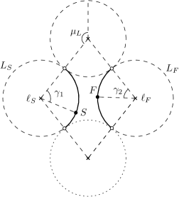
(a) $0\leqslant\gamma_{1},\gamma_{2}\leqslant 2\mu_{\text{\tiny L}}-\pi$

(b) Completing to a loop

Figure 16: Proof of Lemma 10 for case A

For $\mathit{RLR}$-paths, we could argue analogously, or we can simply observe that

$$\operatorname{\textsc{rlr}}(\sigma,\delta)=\operatorname{\textsc{lrl}}(\pi-\sigma,\pi-\delta)=4\mu_{\text{\tiny L}}(\pi-\sigma,\pi-\delta)+2(\pi-\delta)-2\pi=4\mu_{\text{\tiny R}}(\sigma,\delta)-2\delta.$$

Assume now that $(\sigma,\delta)\in B$. By Lemma 3, we have $\pi<2\delta\leqslant 2\pi$. By Lemma 9 and Eq. (18) we have

$$2\mu_{\text{\tiny L}}-\pi \leqslant\gamma_{1}<2\pi$$

$$0 \leqslant\gamma_{2}\leqslant 2\mu_{\text{\tiny L}}-\pi$$

Together these imply $-\pi\leqslant\gamma_{1}+\gamma_{2}-2\mu_{\text{\tiny L}}<\pi$. Since $\gamma_{1}+\gamma_{2}-2\mu_{\text{\tiny L}}\equiv 2\delta\pmod{2\pi}$, we must have $\gamma+\gamma_{2}-2\mu_{\text{\tiny L}}=2\delta-2\pi$. It follows that $\operatorname{\textsc{lrl}}(\sigma,\delta)=4\mu_{\text{\tiny L}}+2\delta-2\pi$.

We turn to the $\mathit{RLR}$-path in case B. By Lemma 9 and Eq. (19) we have (here, $\gamma_{1}$ and $\gamma_{2}$ are the right-turning arcs)

$$0 \leqslant\gamma_{1}\leqslant 2\mu_{\text{\tiny R}}-\pi$$

$$2\mu_{\text{\tiny R}}-\pi \leqslant\gamma_{2}<2\pi$$

Together we have $-\pi\leqslant\gamma_{1}+\gamma_{2}-2\mu_{\text{\tiny R}}\leqslant\pi$. Since $-\gamma_{1}-\gamma_{2}+2\mu_{\text{\tiny R}}\equiv 2\delta\pmod{2\pi}$, we must have $-\gamma_{1}+2\mu_{\text{\tiny R}}-\gamma_{2}=2\delta-2\pi$, which shows that $\operatorname{\textsc{rlr}}=\gamma_{1}+2\mu_{\text{\tiny R}}+\gamma_{2}=4\mu_{\text{\tiny R}}-(2\delta-2\pi)=4\mu_{\text{\tiny R}}-2\delta+2\pi$. ∎

Proof of Lemma 12

Proof.

We first prove that for $(\alpha,\beta)\in B^{\Delta}$, the function $\alpha\mapsto\operatorname{\textsc{lrl}}(\alpha,\beta)$ is decreasing. By Lemma 10 we have $\operatorname{\textsc{lrl}}(\alpha,\beta)=4\mu_{\text{\tiny L}}+2\delta-2\pi$ in $B^{\Delta}$. We have $2\delta=\beta-\alpha$, $\mu_{\text{\tiny L}}=\pi-\arcsin({d_{\text{\tiny L}}}/{4})$, $d_{\text{\tiny L}}^{2}=(d-\sin\beta+\sin\alpha)^{2}+(\cos\beta-\cos\alpha)^{2}$ by Eq. (2), and $\frac{\partial\arcsin{x}}{\partial{x}}=\frac{1}{\sqrt{1-x^{2}}}$. Setting $D_{\text{\tiny L}}=d_{\text{\tiny L}}\sqrt{1-({d_{\text{\tiny L}}/4})^{2}}$, we have

$$\frac{\partial\operatorname{\textsc{lrl}}}{\partial\alpha}(\alpha,\beta) =-\frac{(d-\sin\beta+\sin\alpha)\cos\alpha+(\cos\beta-\cos\alpha)\sin\alpha}{D_{L}}-1.$$

We also have

$$(d-\sin\beta+\sin\alpha)\cos\alpha+(\cos\beta-\cos\alpha)\sin\alpha= d\cos\alpha-\sin\beta\cos\alpha+\cos\beta\sin\alpha$$

$$= d\cos\alpha-\sin(\beta-\alpha)\geqslant 0.$$

The last inequality holds since $0\leqslant\alpha\leqslant\pi/2$ and $\beta-\alpha\geqslant\pi$ in $B^{\Delta}$ by Lemma 3. It follows that $\frac{\partial\operatorname{\textsc{lrl}}}{\partial\alpha}(\alpha,\beta)\leqslant-1<0$.

We now prove that if $(\alpha,\beta)\in B^{\Delta}$ and $\beta\geqslant 3\pi/2$ then $\frac{\partial\operatorname{\textsc{lrl}}}{\partial\beta}(\alpha,\beta)\geqslant 1$. We have

$$\frac{\partial\operatorname{\textsc{lrl}}}{\partial\beta}(\alpha,\beta) =\frac{(d-\sin\beta+\sin\alpha)\cos\beta+(\cos\beta-\cos\alpha)\sin\beta}{D_{L}}+1.$$

$\beta\geqslant{3\pi}/{2}$ implies that $\sin\beta\leqslant 0$ and $\cos\beta\geqslant 0$. By Lemma 3 we have $\pi+\alpha\leqslant\beta\leqslant 2\pi-\alpha$, which implies that $\cos\beta\leqslant\cos\alpha$. It follows that the first term of $\frac{\partial\operatorname{\textsc{lrl}}}{\partial\beta}(\alpha,\beta)$ is nonnegative, proving that $\frac{\partial\operatorname{\textsc{lrl}}}{\partial\beta}(\alpha,\beta)\geqslant 1$.

We finally prove that for $(\alpha,\beta)\in A^{\Delta}\cup B^{\Delta}$ the function $\beta\mapsto\operatorname{\textsc{lrl}}(\alpha,\beta)$ is increasing. Let $U=d-\sin\beta+\sin\alpha$, and $V=\cos\beta-\cos\alpha$ (note that $d_{\text{\tiny L}}^{2}=U^{2}+V^{2}$). If $U\cos\beta+V\sin\beta\geqslant 0$, we have $\frac{\partial\operatorname{\textsc{lrl}}}{\partial\beta}(\alpha,\beta)>0$, and $\beta\mapsto\operatorname{\textsc{lrl}}(\alpha,\beta)$ is increasing. Now let us assume that $U\cos\beta+V\sin\beta$ is negative, and let us compare the squared terms of $\frac{\partial\operatorname{\textsc{lrl}}}{\partial\beta}$ (we only consider the numerator since the denominator is always positive).

$$(U\cos\beta+V\sin\beta)^{2}-d_{\text{\tiny L}}^{2}\!\left({1-\frac{d_{\text{\tiny L}}^{2}}{16}}\right)= (U^{2}\cos^{2}\beta+V^{2}\sin^{2}\beta+2UV\cos\beta\sin\beta)-(U^{2}+V^{2})+\frac{(U^{2}+V^{2})^{2}}{16}$$

$$= (-U^{2}\sin^{2}\beta-V^{2}\cos^{2}\beta+2UV\cos\beta\sin\beta)+\frac{(U^{2}+V^{2})^{2}}{16}$$

$$= \frac{1}{16}\!\left({-16(U\sin\beta-V\cos\beta)^{2}+(U^{2}+V^{2})^{2}}\right).$$

For $(\alpha,\beta)\in A^{\Delta}\cup B^{\Delta}$, we have $d_{\text{\tiny LR}}<2$. From Eq. (4), $d_{\text{\tiny LR}}^{2}=(d+\sin\beta+\sin\alpha)^{2}+(\cos\beta+\cos\alpha)^{2}<4$. By substituting $d+\sin\alpha=U+\sin\beta$ and $\cos\alpha=\cos\beta-V$, we have

$$d_{\text{\tiny LR}}^{2}<4$$

$$\Leftrightarrow(U+2\sin\beta)^{2}+(2\cos\beta-V)^{2}<4$$

$$\Leftrightarrow U^{2}+V^{2}+4(U\sin\beta-V\cos\beta)+4(\sin^{2}\beta+\cos^{2}\beta)<4$$

$$\Leftrightarrow(U^{2}+V^{2})+4(U\sin\beta-V\cos\beta)<0.$$

Since $U^{2}+V^{2}=d_{\text{\tiny L}}^{2}\geqslant 0$, this implies that $U\sin\beta-V\cos\beta<0$, and further the squared term $16(U\sin\beta-V\cos\beta)^{2}$ is greater than $(U^{2}+V^{2})^{2}$, which implies that $(U^{2}+V^{2})^{2}-16(U\sin\beta-V\cos\beta)^{2}<0$, completing the proof. ∎

Proof of Lemma 13

Proof.

Setting $D_{\text{\tiny L}}=d_{\text{\tiny L}}\sqrt{1-({d_{\text{\tiny L}}/4})^{2}}$ and $D_{\text{\tiny R}}=d_{\text{\tiny R}}\sqrt{1-({d_{\text{\tiny R}}/4})^{2}}$, we obtain the derivatives of l and r using $\mu_{\text{\tiny L}}=\pi-\arcsin({d_{\text{\tiny L}}}/{4})$, $\mu_{\text{\tiny R}}=\pi-\arcsin({d_{\text{\tiny R}}}/{4})$, and Eqns. (6)–(9):

$$\frac{\partial\textsc{l}}{\partial\delta}(\sigma,\delta) =2+\frac{-4\cos\delta\sin\delta+2d\cos\delta\cos\sigma}{D_{\text{\tiny L}}},$$ (20)

$$\frac{\partial\textsc{l}}{\partial\sigma}(\sigma,\delta) =\frac{-2d\sin\delta\sin\sigma}{D_{\text{\tiny L}}},$$ (21)

$$\frac{\partial\textsc{r}}{\partial\delta}(\sigma,\delta) =-2+\frac{-4\cos\delta\sin\delta-2d\cos\delta\cos\sigma}{D_{\text{\tiny R}}},$$ (22)

$$\frac{\partial\textsc{r}}{\partial\sigma}(\sigma,\delta) =\frac{2d\sin\delta\sin\sigma}{D_{\text{\tiny R}}}.$$ (23)

The derivatives are not defined when $D_{\text{\tiny L}}=0$ or $D_{\text{\tiny R}}=0$. $D_{\text{\tiny L}}=0$ occurs when $d_{\text{\tiny L}}=0$ or $d_{\text{\tiny L}}=4$, and $D_{\text{\tiny R}}=0$ occurs when $d_{\text{\tiny R}}=0$ or $d_{\text{\tiny R}}=4$.

In the interior of $\Xi$, we have $\sin\delta>d/2$, which implies $\cos\delta^{2}<1-d^{2}/4$. So for $\alpha^{\ast}<\delta\leqslant\pi/2$, we have $d_{\text{\tiny RL}}<2$ by Eq. (9), and for $\pi/2\leqslant\delta<\pi-\alpha^{\ast}$, we have $d_{\text{\tiny LR}}<2$ by Eq. (8). By the triangle inequality it follows that $d_{\text{\tiny L}}<4$ and $d_{\text{\tiny R}}<4$. Also, by Eq. (6) $d_{\text{\tiny L}}^{2}=(d-2\sin\delta\cos\sigma)^{2}+4\sin\delta(-\cos\sigma+1)$. Since $\sin\delta>0$, $d_{\text{\tiny L}}=0$ can occur only when $\sigma=0$ and $\delta\in\{\alpha^{\ast},\pi-\alpha^{\ast}\}$, which occurs at a corner of $\Xi$. Similar arguments hold for the case where $d_{\text{\tiny R}}^{2}=0$. Thus, in the interior of $\Xi$, $D_{\text{\tiny L}}\neq 0$ and $D_{\text{\tiny R}}\neq 0$.

Consider Eqns. (21) and (23). Since $\sin\delta>0$ in $\Xi$ and $\sin\sigma\geqslant 0$ with equality only for $\sigma\in\{0,\pi\}$, we have $\frac{\partial\textsc{l}}{\partial\sigma}<0$ and $\frac{\partial\textsc{r}}{\partial\sigma}>0$ in the interior of $\Xi$.

It remains to discuss the two functions of $\delta$. We show that $\frac{\partial\textsc{l}}{\partial\delta}(\sigma,\delta)>0$. If $Z=2\cos\delta(-2\sin\delta+d\cos\sigma)\geqslant 0$, this is true. Let us thus assume that $Z<0$. Since $\sin\delta\geqslant d/2$ implies that $-2\sin\delta+d\cos\sigma\leqslant-2(d/2)+d\cos\sigma=d(-1+\cos\sigma)\leqslant 0$, we have $\cos\delta>0$ and so $-2\sin\delta+d\cos\sigma<0$. $\sin\delta\geqslant d/2$ also implies that $d^{2}\leqslant 4\sin^{2}\delta$, so by Eq. (6) $d_{\text{\tiny L}}^{2}=d^{2}-4d\sin\delta\cos\sigma+4\sin^{2}\delta\leqslant 8\sin^{2}\delta-4d\sin\delta\cos\sigma=4\sin\delta(2\sin\delta-d\cos\sigma)$. Since $d_{\text{\tiny L}}^{2}\geqslant 0$, we have

$$d_{\text{\tiny L}}^{4}\leqslant 16\sin^{2}\delta(2\sin\delta-d\cos\sigma)^{2}.$$ (24)

On the other hand, we have

$$d_{\text{\tiny L}}^{2} =d^{2}-4d\sin\delta\cos\sigma+4\sin^{2}\delta$$

$$\geqslant d^{2}\cos^{2}\sigma-4d\sin\delta\cos\sigma+4\sin^{2}\delta=(2\sin\delta-d\cos\sigma)^{2}.$$ (25)

Now we want to show that $2D_{\text{\tiny L}}\geqslant-Z$, which will imply $\frac{\partial\textsc{l}}{\partial\delta}(\sigma,\delta)\geqslant 0$. Let us compare the squared terms:

$$4{D_{\text{\tiny L}}}^{2}-Z^{2}$$

$$=4D_{\text{\tiny L}}^{2}-4\cos^{2}\delta(-2\sin\delta+d\cos\sigma)^{2}$$

$$=4\!\left({d_{\text{\tiny L}}^{2}\!\left({1-\frac{d_{\text{\tiny L}}^{2}}{16}}\right)-\cos^{2}\delta(2\sin\delta-d\cos\sigma)^{2}}\right)$$

$$\geqslant 4\!\left({d_{\text{\tiny L}}^{2}-\sin^{2}\delta(2\sin\delta-d\cos\sigma)^{2}-\cos^{2}\delta(2\sin\delta-d\cos\sigma)^{2}}\right)\quad\text{(by~{}\eqref{eq:dl-smaller})}$$

$$=4\!\left({d_{\text{\tiny L}}^{2}-(2\sin\delta-d\cos\sigma)^{2}}\right)\geqslant 0\quad\text{(by~{}\eqref{eq:dl-larger})}.$$

One of the inequalities in above formula is a strict inequality: if (A) is an equality, then $d_{\text{\tiny L}}^{2}=(2\sin\delta-d\cos\sigma)^{2}$, which means that $\cos^{2}\sigma=1$. This implies that $d^{2}<4\sin^{2}\delta$ since we have $-2\sin\delta+d\cos\sigma<0$, so (24) is strict. In the case where (24) is an equality, we can argue similarly that (A) is strict.

Similarly, we prove that $\frac{\partial\textsc{r}}{\partial\delta}(\sigma,\delta)<0$, since $\sin\delta\geqslant d/2$ again implies that $d_{\text{\tiny R}}^{2}=d^{2}+4d\sin\delta\cos\sigma+4\sin^{2}\delta\leqslant 4\sin\delta(2\sin\delta+d\cos\sigma)$, so

$$d_{\text{\tiny R}}^{4} \leqslant 16\sin^{2}\delta(2\sin\delta+d\cos\sigma)^{2},$$

and we have

$$d_{\text{\tiny R}}^{2} \geqslant d^{2}\cos^{2}\sigma+4d\sin\delta\cos\sigma+4\sin^{2}\delta=(2\sin\delta+d\cos\sigma)^{2}.\qed$$

Proof of Lemma 14

Proof.

By Lemma 13, neither l nor r has a local extremum in the interior of $\Xi$, so any local extremum of $\textsc{c}(\sigma,\delta)$ must be a point in the set $\Lambda$ of points $(\sigma,\delta)$ with $\textsc{l}(\sigma,\delta)=\textsc{r}(\sigma,\delta)$. By Lemma 13, $\Lambda$ is a $\delta$-monotone curve. Since $\textsc{l}(\sigma,\delta)=\textsc{r}(\pi-\sigma,\pi-\delta)$, the curve $\Lambda$ passes through the point $(\pi/2,\pi/2)$. By Lemma 13, this implies that $\textsc{l}(\sigma,\delta)<\textsc{r}(\sigma,\delta)$ for the quadrant $\pi/2\leqslant\sigma\leqslant\pi$, $\alpha^{\ast}\leqslant\delta\leqslant\pi/2$, and that $\textsc{r}(\sigma,\delta)<\textsc{l}(\sigma,\delta)$ for the quadrant $0\leqslant\sigma\leqslant\pi/2$, $\pi/2\leqslant\delta\leqslant\pi-\alpha^{\ast}$ except at the point $(\pi/2,\pi/2)$. By point symmetry, we can restrict our attention to the range $\pi/2<\sigma<\pi$, $\pi/2<\delta<\pi-\alpha^{\ast}$.

Assume for a contradiction that $(\sigma,\delta)\in\Lambda$ is a local extremum of l, restricted to $\Lambda$. This implies that the gradient $\nabla\textsc{l}(\sigma,\delta)$ and the normal of $\Lambda$ in $(\sigma,\delta)$ are linearly dependent, by the method of Lagrange Multipliers. The normal of $\Lambda$ is the gradient of $\textsc{l}(\sigma,\delta)-\textsc{r}(\sigma,\delta)$, so $\nabla\textsc{l}(\sigma,\delta)$ and $\nabla\textsc{r}(\sigma,\delta)$ must be linearly dependent.

For the two vectors to be linearly dependent, we would have to have

$$D_{\text{\tiny L}}\frac{\partial\textsc{l}}{\partial\delta}(\sigma,\delta)+D_{\text{\tiny R}}\frac{\partial\textsc{r}}{\partial\delta}(\sigma,\delta)=0,$$

which means

$$2D_{\text{\tiny L}}-2D_{\text{\tiny R}}-8\cos\delta\sin\delta=0.$$

In the range under consideration, $-8\cos\delta\sin\delta>0$. We will show that $D_{\text{\tiny L}}>D_{\text{\tiny R}}$, a contradiction. We have

$$16(D_{\text{\tiny L}}^{2}-D_{\text{\tiny R}}^{2}) =d_{\text{\tiny L}}^{2}(16-d_{\text{\tiny L}}^{2})-d_{\text{\tiny R}}^{2}(16-d_{\text{\tiny R}}^{2})$$

$$=d_{\text{\tiny R}}^{4}-d_{\text{\tiny L}}^{4}+16(d_{\text{\tiny L}}^{2}-d_{\text{\tiny R}}^{2})$$

$$=(d_{\text{\tiny L}}^{2}-d_{\text{\tiny R}}^{2})(16-(d_{\text{\tiny L}}^{2}+d_{\text{\tiny R}}^{2}))$$

$$=-8d\cos\sigma\sin\delta(16-(2d^{2}+8\sin^{2}\delta)).$$

Since $\cos\sigma<0$ and $d<2$, the expression is positive. ∎

Proof of Lemma 16

Proof.

We will show below that the two functions $d\mapsto\textsc{a}(d)$ and $d\mapsto\textsc{a}(d)-d$ have no extremum on the interval $(0,\sqrt{2})$. This will imply the claim if we observe that

$$\textsc{a}(0) =7\pi/3,$$

$$\textsc{a}(\sqrt{2}) =5\pi/2>\textsc{a}(0)$$

$$\textsc{a}(\sqrt{2})-\sqrt{2} =5\pi/2-\sqrt{2}<\textsc{a}(0)-0.$$

Again we will employ Lagrange multipliers. Let us first give the necessary derivatives. Setting $\sigma=\pi$ and $\pi/2<\delta\leqslant\pi-\alpha^{\ast}$ (by Lemma 15), we have:

$$d_{\text{\tiny L}} =d+2\sin\delta\qquad\text{by (\ref{eq:dl-sigma-delta})}$$

$$d_{\text{\tiny R}} =2\sin\delta-d\qquad\text{by (\ref{eq:dr-sigma-delta})}$$

$$\textsc{l}(d,\pi,\delta) =2\pi-4\arcsin(d_{\text{\tiny L}}/4)+2\delta\qquad\text{by (\ref{eq:def-l})}$$

$$\textsc{r}(d,\pi,\delta) =4\pi-4\arcsin(d_{\text{\tiny R}}/4)-2\delta\qquad\text{by (\ref{eq:def-r})}$$

Let us introduce $F_{\text{\tiny L}}=\sqrt{1-(d_{\text{\tiny L}}/4)^{2}}$ and $F_{\text{\tiny R}}=\sqrt{1-(d_{\text{\tiny R}}/4)^{2}}$ to obtain:

$$\frac{\partial}{\partial d}\textsc{l}(d,\pi,\delta) =-\frac{1}{F_{\text{\tiny L}}}\qquad\frac{\partial}{\partial\delta}\textsc{l}(d,\pi,\delta)=2-\frac{2\cos\delta}{F_{\text{\tiny L}}}$$

$$\frac{\partial}{\partial d}\textsc{r}(d,\pi,\delta) =\frac{1}{F_{\text{\tiny R}}}\qquad\frac{\partial}{\partial\delta}\textsc{r}(d,\pi,\delta)=-2-\frac{2\cos\delta}{F_{\text{\tiny R}}}$$

We consider first the function $d\mapsto\textsc{a}(d)$. An extremum of $\textsc{a}(d)$ is an extremum of the two-parameter function $(d,\delta)\mapsto\textsc{l}(d,\pi,\delta)$ under the restriction $\textsc{l}(d,\pi,\delta)=\textsc{r}(d,\pi,\delta)$. Such an extremum would have to satisfy the condition $\nabla\textsc{l}(d,\pi,\delta)=\lambda\nabla\textsc{r}(d,\pi,\delta)$. For this to hold:

$$\lambda=-\frac{F_{\text{\tiny R}}}{F_{\text{\tiny L}}} =\frac{2-2\cos\delta/F_{\text{\tiny L}}}{-2-2\cos\delta/F_{\text{\tiny R}}},$$

which implies $F_{\text{\tiny R}}-F_{\text{\tiny L}}=-2\cos\delta$. Since $d_{\text{\tiny R}}<2$, $F_{\text{\tiny R}}>\sqrt{3}/2$, and since $d_{\text{\tiny L}}<2+\sqrt{2}<2\sqrt{3}$, $F_{\text{\tiny L}}>1/2$. This implies $F_{\text{\tiny R}}+F_{\text{\tiny L}}>1$, and so

$$-2\cos\delta=F_{\text{\tiny R}}-F_{\text{\tiny L}}<(F_{\text{\tiny R}}-F_{\text{\tiny L}})(F_{\text{\tiny R}}+F_{\text{\tiny L}})=F_{\text{\tiny R}}^{2}-F_{\text{\tiny L}}^{2}=\frac{d}{2}\sin\delta.$$ (26)

The condition $\textsc{l}(d,\pi,\delta)=\textsc{r}(d,\pi,\delta)$ implies (using $\arcsin x-\arcsin y\geqslant x-y$ for $0\leqslant y\leqslant x\leqslant 1$)

$$4\delta=2\pi+4\big{(}\arcsin\frac{d_{\text{\tiny L}}}{4}-\arcsin\frac{d_{\text{\tiny R}}}{4}\big{)}\geqslant 2\pi+(d_{\text{\tiny L}}-d_{\text{\tiny R}})=2\pi+2d.$$

It follows that $\pi/2+d/2\leqslant\delta\leqslant\pi$, and so we have $\sin\delta\leqslant\cos\frac{d}{2}$ and $-\cos\delta\geqslant\sin\frac{d}{2}$. With (26) this gives

$$2\sin\frac{d}{2}\leqslant-2\cos\delta<\frac{d}{2}\sin\delta\leqslant\frac{d}{2}\cos\frac{d}{2}.$$

Setting $f(x):=x\cos x-2\sin x$, this implies $f(d/2)>0$. But this is impossible, since $f(0)=0$ and $f^{\prime}(x)=-2\cos x-x\sin x\leqslant 0$ for $0\leqslant x\leqslant d/2<\pi/2$.

Consider next the function $d\mapsto\textsc{a}(d)-d$. An extremum of $\textsc{a}(d)-d$ is an extremum of the two-parameter function $(d,\delta)\mapsto\textsc{l}(d,\pi,\delta)-d$ under the restriction $\textsc{l}(d,\pi,\delta)=\textsc{r}(d,\pi,\delta)$. Such an extremum would have to satisfy the condition $\lambda\nabla(\textsc{l}(d,\pi,\delta)-d)=\nabla\big{(}\textsc{l}(d,\pi,\delta)-\textsc{r}(d,\pi,\delta)\big{)}$, or

$$\lambda(-\frac{1}{F_{\text{\tiny L}}}-1) =-\frac{1}{F_{\text{\tiny L}}}-\frac{1}{F_{\text{\tiny R}}},$$

$$\lambda(2-\frac{2\cos\delta}{F_{\text{\tiny L}}}) =4-\frac{2\cos\delta}{F_{\text{\tiny L}}}+\frac{2\cos\delta}{F_{\text{\tiny R}}}$$

The two components give us the following conditions on $\lambda$:

$$\lambda =1+\frac{1/F_{\text{\tiny R}}-1}{1/F_{\text{\tiny L}}+1}=1+\frac{2+(2\cos\delta)/F_{\text{\tiny R}}}{2-(2\cos\delta)/F_{\text{\tiny L}}}.$$

This is equivalent to

$$\Big{(}2-\frac{2\cos\delta}{F_{\text{\tiny L}}}\Big{)}\Big{(}\frac{1}{F_{\text{\tiny R}}}-1\Big{)} =\Big{(}2+\frac{2\cos\delta}{F_{\text{\tiny R}}}\Big{)}\Big{(}\frac{1}{F_{\text{\tiny L}}}+1\Big{)}.$$

Multiplying out and rearranging the terms gives

$$(2-2\cos\delta)\Big{(}\frac{1}{F_{\text{\tiny R}}}-\frac{1}{F_{\text{\tiny L}}}\Big{)} =4\Big{(}\frac{\cos\delta}{F_{\text{\tiny R}}F_{\text{\tiny L}}}+1\Big{)}.$$

Since $d_{\text{\tiny L}}-d_{\text{\tiny R}}=2d>0$, we have $F_{\text{\tiny R}}>F_{\text{\tiny L}}$. With $\cos\delta<0$ this implies that the left-hand side is negative. We will now show that the right-hand side is non-negative, a contradiction, and so $d\mapsto\textsc{a}(d)-d$ cannot have a local extremum.

It is enough to show that $\cos^{2}\delta\leqslant(F_{\text{\tiny R}}F_{\text{\tiny L}})^{2}$:

$$(F_{\text{\tiny R}}F_{\text{\tiny L}})^{2}-\cos^{2}\delta =\Big{(}1-\frac{d_{\text{\tiny L}}^{2}+d_{\text{\tiny R}}^{2}}{16}+\frac{(d_{\text{\tiny L}}d_{\text{\tiny R}})^{2}}{16^{2}}\Big{)}-\cos^{2}\delta$$

$$=-\frac{2d^{2}+8\sin^{2}\delta}{16}+\frac{(d_{\text{\tiny L}}d_{\text{\tiny R}})^{2}}{16^{2}}+\sin^{2}\delta$$

$$=\frac{-2d^{2}+8\sin^{2}\delta}{16}+\frac{(d_{\text{\tiny L}}d_{\text{\tiny R}})^{2}}{16^{2}}\geqslant 0.$$

The last inequality holds since $\sin\delta\geqslant d/2$. ∎

Proof of Lemma 21

Proof.

The two derivatives in Eqns. (15) and (16) are defined and both positive in the interior of $B^{\circ}$, implying the first two claims.

For the third claim, we need to show that

$$0 \leqslant\frac{\partial}{\partial\alpha}\operatorname{\textsc{rsl}}(\alpha,\beta)-\frac{\partial}{\partial\beta}\operatorname{\textsc{rsl}}(\alpha,\beta)=-\cos\gamma_{\text{\tiny R}}+\cos\gamma_{\text{\tiny L}}$$

for $\beta=2\pi-\alpha$. By Lemma 9, $S$ lies on the arc $\ddddot{S^{\text{\tiny L}}_{0}S^{\text{\tiny L}}_{1}}$ of $L_{S}$. If $\beta=2\pi-\alpha$, then $F$ lies on the counter-clockwise arc $\ddddot{F^{\text{\tiny L}}_{1}F^{\text{\tiny L}}_{0}}$ of $L_{F}$. The two circular arcs of the $\mathit{RSL}$-path have two components, namely, $\gamma_{\text{\tiny R}}=\alpha+\zeta$ and $\gamma_{\text{\tiny L}}=\beta+\zeta=2\pi-\alpha+\zeta$, see Figure 17. This implies

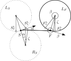
Figure 17: An $\mathit{RSL}$-path for $\beta=2\pi-\alpha$

$$-\cos\gamma_{\text{\tiny R}}+\cos\gamma_{\text{\tiny L}} =-\cos(\alpha+\zeta)+\cos(\alpha-\zeta)=2\sin\alpha\sin{\zeta}\geqslant 0.$$

The second and third claim immediately imply the last one. ∎

Proof of Lemma 22

Proof.

We first compare the $\mathit{LRL}$-path and the $\mathit{LSL}$-path. Let $\gamma_{1}$ and $\gamma_{2}$ be the two arcs on the $\mathit{LRL}$-path. By Lemma 9, we have $2\mu_{\text{\tiny L}}-\pi\leqslant\gamma_{1}\leqslant\mu_{\text{\tiny L}}$ and $0\leqslant\gamma_{2}\leqslant 2\mu_{\text{\tiny L}}-\pi$. The $\mathit{LSL}$-path has length $\operatorname{\textsc{lsl}}=\gamma_{1}+\gamma_{2}+2(2\pi-\mu_{\text{\tiny L}})+d_{\text{\tiny L}}$. We thus have $\operatorname{\textsc{lsl}}-\operatorname{\textsc{lrl}}=d_{\text{\tiny L}}+4(\pi-\mu_{\text{\tiny L}})\geqslant 0$.

Consider now the $\mathit{LRL}$-path and the $\mathit{RLR}$-path. By (6) and (7), we have $d_{\text{\tiny R}}^{2}-d_{\text{\tiny L}}^{2}=8d\sin\delta\cos\sigma\leqslant 0$ for $(\sigma,\delta)\in B^{\Delta}$, and so $d_{\text{\tiny R}}\leqslant d_{\text{\tiny L}}$, implying $\mu_{\text{\tiny L}}\leqslant\mu_{\text{\tiny R}}$. By Lemma 10, we have $\operatorname{\textsc{rlr}}-\operatorname{\textsc{lrl}}=4(\mu_{\text{\tiny R}}-\mu_{\text{\tiny L}}-\delta+\pi)\geqslant 0$.

Finally, we compare $\mathit{RSL}$-path and $\mathit{RSR}$-path. The $\mathit{RSL}$-path consist of an initial right-turning arc $\ddddot{ST_{S}}$, a segment $\overline{T_{S}T_{F}}$, and a final left-turning arc $\ddddot{T_{F}F}$. The $\mathit{RSR}$-path consist of an initial right-turning arc $\ddddot{SR_{1}}$, a segment $\overline{R_{1}R_{2}}$, and a final right-turning arc $\ddddot{R_{2}F}$, see Figure 18.

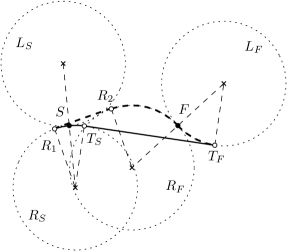
Figure 18: $\operatorname{\textsc{rsl}}(\alpha,\beta)\leqslant\operatorname{\textsc{rsr}}(\alpha,\beta)$ for $(\alpha,\beta)\in B^{\Delta}$ with $\beta$ close to $\beta_{\text{\tiny LR}}(\alpha)$.

We first claim that the arc $\ddddot{ST_{S}}$ is common to both paths. Indeed, since $d_{\text{\tiny LR}}<2$, by Lemma 9, the initial arc $\ddddot{SR_{1}}$ of the $\mathit{RSR}$-path must have length at least $\pi$ (Figure 13(b)), while the arc $\ddddot{ST_{S}}$ must be shorter than $\pi$ (Figure 13(a)).

Since $|\ddddot{T_{F}F}|=2\pi-|\ddddot{FT_{F}}|$ and $|\ddddot{T_{S}R_{1}}|=2\pi-|\ddddot{R_{1}T_{S}}|$, where $\ddddot{FT_{F}}$ is a left-turning arc on the disk $L_{F}$ and $\ddddot{R_{1}T_{S}}$ is a right-turning arc on disk $R_{S}$, we have

$$\operatorname{\textsc{rsl}}-\operatorname{\textsc{rsr}} =\big{(}|\overline{T_{S}T_{F}}|-|\ddddot{FT_{F}}|\big{)}-\big{(}-|\ddddot{R_{1}T_{S}}|+|\overline{R_{1}R_{2}}|+|\ddddot{R_{2}F}|\big{)}$$

$$=|\ddddot{R_{1}T_{S}}\cup\overline{T_{S}T_{F}}|-|\overline{R_{1}R_{2}}\cup\ddddot{R_{2}F}\cup\ddddot{FT_{F}}|.$$

The path $\overline{R_{1}R_{2}}\cup\ddddot{R_{2}f}\cup\ddddot{FT_{F}}$ is a path connecting $R_{1}$ with $T_{F}$ while avoiding the interior of $R_{S}$. However, the path $\ddddot{R_{1}T_{S}}\cup\overline{T_{S}T_{F}}$ is clearly the shortest path of this kind, and so $\operatorname{\textsc{rsl}}-\operatorname{\textsc{rsr}}\leqslant 0$. ∎

Proof of Lemma 23

Proof.

We first observe that the function $\alpha\mapsto\operatorname{\textsc{lrl}}(\alpha,\beta)-\operatorname{\textsc{rsl}}(\alpha,\beta)$ is decreasing. This follows immediately from Lemmas 21 and 12. We also claim that the function $\beta\mapsto\operatorname{\textsc{lrl}}(\alpha,\beta)-\operatorname{\textsc{rsl}}(\alpha,\beta)$ is increasing for $\beta\geqslant 3\pi/2$. Together, these facts prove the lemma: consider two values $0\leqslant\alpha_{1}<\alpha_{2}\leqslant\alpha^{\ast}$. Since $\beta_{\text{\tiny LR}}(\alpha)$ is a decreasing function, we have $\beta_{\text{\tiny LR}}(\alpha_{1})>\beta_{\text{\tiny LR}}(\alpha_{2})\geqslant 2\pi-\alpha^{\ast}>3\pi/2$, and so

$$\operatorname{\textsc{lrl}}(\alpha_{1},\beta_{\text{\tiny LR}}(\alpha_{1}))-\operatorname{\textsc{rsl}}(\alpha_{1},\beta_{\text{\tiny LR}}(\alpha_{1})) \geqslant\operatorname{\textsc{lrl}}(\alpha_{1},\beta_{\text{\tiny LR}}(\alpha_{2}))-\operatorname{\textsc{rsl}}(\alpha_{1},\beta_{\text{\tiny LR}}(\alpha_{2}))$$

$$\geqslant\operatorname{\textsc{lrl}}(\alpha_{2},\beta_{\text{\tiny LR}}(\alpha_{2}))-\operatorname{\textsc{rsl}}(\alpha_{2},\beta_{\text{\tiny LR}}(\alpha_{2})).$$

It remains to show that for $(\alpha,\beta)\in B^{\Delta}$ with $\beta\geqslant{3\pi}/{2}$, the function $\beta\mapsto\operatorname{\textsc{lrl}}(\alpha,\beta)-\operatorname{\textsc{rsl}}(\alpha,\beta)$ is increasing. Since we are in case $B^{\Delta}$, by Lemma 9 the point $S$ lies on the arc $\ddddot{S^{\text{\tiny L}}_{0}S^{\text{\tiny L}}_{1}}$ of $L_{S}$, while $F$ lies on the arc $\ddddot{F^{\text{\tiny L}}_{2}F^{\text{\tiny L}}_{1}}$ of $L_{F}$ (see Figure 13(a)). It follows that $\gamma_{\text{\tiny L}}>\beta\geqslant 3\pi/2$, and so $\cos\gamma_{\text{\tiny L}}>0$. This implies that $\frac{\partial}{\partial\beta}\operatorname{\textsc{rsl}}(\alpha,\beta)=1-\cos\gamma_{\text{\tiny L}}<1$. On the other hand, by Lemma 12, $\frac{\partial}{\partial\beta}\operatorname{\textsc{lrl}}(\alpha,\beta)\geqslant 1$ for $\beta\geqslant{3\pi}/{2}$, and the claim follows. ∎

Proof of Lemma 24

Proof.

We first claim that for $(\alpha,\beta)\in B^{\circ}$ and $d<2$, if $\gamma_{\text{\tiny R}}+\gamma_{\text{\tiny L}}\leqslant 2\pi$, then $\operatorname{\textsc{rsl}}(d,\alpha,\beta)\leqslant d+2\pi$.

Let $T_{S}$ and $T_{F}$ denote the points of tangency of the $S$-segment to $R_{S}$ and $L_{F}$. We observed above that $\gamma_{\text{\tiny R}}\leqslant\pi$. If we also have $\gamma_{\text{\tiny L}}\leqslant\pi$ then $d\geqslant|T_{S}T_{F}|$, and the claim follows immediately.

If $\gamma_{\text{\tiny R}}\geqslant\pi/2$, then we have $\gamma_{\text{\tiny L}}\leqslant 2\pi-\gamma_{\text{\tiny R}}\leqslant 3\pi/2$. But then $d=|SF|\geqslant 2$, a contradiction. It follows that we must have $\gamma_{\text{\tiny R}}<\pi/2$. See Figure 19.

Figure 19: If $\gamma_{\text{\tiny R}}+\gamma_{\text{\tiny L}}\leqslant 2\pi$ then $\operatorname{\textsc{rsl}}\leqslant d+2\pi$

Let $S^{\prime}$ be the point on $L_{F}$ such that the counter-clockwise arc $\ddddot{S^{\prime}T_{F}}$ on $L_{F}$ has length $\gamma_{\text{\tiny R}}$. Let $h_{S}$ and $h_{S^{\prime}}$ be lines through $S$ and $S^{\prime}$ orthogonal to the segment $\overline{T_{S}T_{F}}$. The distance between $h_{S}$ and $h_{S^{\prime}}$ is $|T_{S}T_{F}|$, and so we have $|SS^{\prime}|\geqslant|T_{S}T_{F}|$. By the triangle inequality, we have $d+|\ddddot{FS^{\prime}}|=|SF|+|\ddddot{FS^{\prime}}|\geqslant|SS^{\prime}|\geqslant|T_{S}T_{F}|$, so $|T_{S}T_{F}|-|\ddddot{FS^{\prime}}|\leqslant d$. Since $2\pi-|\ddddot{FS^{\prime}}|=\gamma_{\text{\tiny R}}+\gamma_{\text{\tiny L}}$, we have

$$\operatorname{\textsc{rsl}}(d,\alpha,\beta)=\gamma_{\text{\tiny R}}+|T_{S}T_{F}|+\gamma_{\text{\tiny L}}=|T_{S}T_{F}|+2\pi-|\ddddot{FS^{\prime}}|\leqslant d+2\pi,$$

and the claim follows.

Now let $\alpha_{0}$ be such an extremum, and consider the $\mathit{RSL}$-path for $(\alpha_{0},\beta_{\text{\tiny LR}}(\alpha_{0}))$. If $\gamma_{\text{\tiny R}}+\gamma_{\text{\tiny L}}\leqslant 2\pi$, then by above argument we have $\operatorname{\textsc{rsl}}(d,\alpha_{0},\beta_{\text{\tiny LR}}(\alpha_{0}))\leqslant d+2\pi$. We can therefore assume $\gamma_{\text{\tiny R}}+\gamma_{\text{\tiny L}}>2\pi$. The point $(\alpha_{0},\beta_{\text{\tiny LR}}(\alpha_{0}))$ is an extremum of the function $\operatorname{\textsc{rsl}^{\ast}}(\alpha,\beta)$, under the constraint that $d_{\text{\tiny LR}}^{2}=4$, and so there must be a constant $\lambda$ such that $\nabla\operatorname{\textsc{rsl}^{\ast}}(\alpha_{0},\beta_{\text{\tiny LR}}(\alpha_{0}))=\lambda\nabla d_{\text{\tiny LR}}^{2}(\alpha_{0},\beta_{\text{\tiny LR}}(\alpha_{0}))$.

Using $\pi/2<\sigma,\delta\leqslant\pi$ and (8) we have

$$\frac{\partial}{\partial\sigma}d_{\text{\tiny LR}}^{2} =4d\cos\delta\cos\sigma>0$$ (27)

$$\frac{\partial}{\partial\delta}d_{\text{\tiny LR}}^{2} =-4\sin\delta(d\sin\sigma+2\cos\delta).$$ (28)

Using (15) and (16) we get

$$2\frac{\partial}{\partial\sigma}\operatorname{\textsc{rsl}^{\ast}} =\frac{\partial}{\partial\beta}\operatorname{\textsc{rsl}^{\ast}}+\frac{\partial}{\partial\alpha}\operatorname{\textsc{rsl}^{\ast}}=2-\cos\gamma_{\text{\tiny L}}-\cos\gamma_{\text{\tiny R}}\geqslant 0$$ (29)

$$2\frac{\partial}{\partial\delta}\operatorname{\textsc{rsl}^{\ast}} =\frac{\partial}{\partial\beta}\operatorname{\textsc{rsl}^{\ast}}-\frac{\partial}{\partial\alpha}\operatorname{\textsc{rsl}^{\ast}}=-\cos\gamma_{\text{\tiny L}}+\cos\gamma_{\text{\tiny R}}.$$ (30)

Inequalities (27) and (29) imply that $\lambda\geqslant 0$, so let us consider (28). By Lemma 7, we have $\sigma+\delta=\beta_{\text{\tiny LR}}(\alpha_{0})\geqslant\beta_{\text{\tiny LR}}(\alpha^{\ast})=2\pi-\alpha^{\ast}>3\pi/2$ for $d<2$, and so $\cos\delta<\cos(3\pi/2-\sigma)=-\sin\sigma$. It follows that $2\cos\delta<-2\sin\sigma<-d\sin\sigma$, and so (28) is positive.

We have $0\leqslant\gamma_{\text{\tiny R}}\leqslant\pi$ and we assumed that $\gamma_{\text{\tiny R}}+\gamma_{\text{\tiny L}}>2\pi$. It follows that $\gamma_{\text{\tiny L}}>2\pi-\gamma_{\text{\tiny R}}\geqslant\pi$. Since $\gamma_{\text{\tiny R}}>2\pi-\gamma_{\text{\tiny L}}$ we have $\cos\gamma_{\text{\tiny R}}<\cos\gamma_{\text{\tiny L}}$. This implies that (30) is negative. But this means that $\lambda<0$, a contradiction. ∎

References

- [1] P. K. Agarwal, T. Biedl, S. Lazard, S. Robbins, S. Suri, and S. Whitesides. Curvature-constrained shortest paths in a convex polygon. SIAM Journal on Computing, 31(6):1814–1851, 2002.
- [2] P. K. Agarwal, P. Raghavan, and H. Tamaki. Motion planning for a steering-constrained robot through moderate obstacles. In Proceedings of the twenty-seventh annual ACM symposium on Theory of computing, pages 343–352, New York, NY, USA, 1995. ACM Press.
- [3] P. K. Agarwal and H. Wang. Approximation algorithms for curvature-constrained shortest paths. SIAM Journal on Computing, 30(6):1739–1772, 2001.
- [4] J. Backer and D. Kirkpatrick. A complete approximation algorithm for shortest bounded-curvature paths. In Proceedings of the nineteenth International Symposium on Algorithms and Computation, pages 628–643, Dec 2008.
- [5] S. Bereg and D. Kirkpatrick. Curvature-bounded traversals of narrow corridors. In Proceedings of the twenty-first annual symposium on Computational Geometry, pages 278–287, New York, NY, USA, 2005. ACM Press.
- [6] J.-D. Boissonnat and X.-N. Bui. Accessibility region for a car that only moves forwards along optimal paths. Research Report 2181, INRIA, Le Chesnay Cedex, France, 1994.
- [7] J.-D. Boissonnat, A. Cérézo, and J. Leblond. Shortest paths of bounded curvature in the plane. Journal of Intelligent and Robotic Systems, 11(1-2):5–20, 1994.
- [8] J.-D. Boissonnat, S. Ghosh, T. Kavitha, and S. Lazard. An algorithm for computing a convex and simple path of bounded curvature in a simple polygon. Algorithmica, 34:109–156, 2002.
- [9] J.-D. Boissonnat and S. Lazard. A polynomial-time algorithm for computing a shortest path of bounded curvature amidst moderate obstacles. International Journal of Computational Geometry and Applications, 13(3):189–229, June 2003.
- [10] X.-N. Bui, P. Souères, J.-D. Boissonnat, and J.-P. Laumond. The shortest paths synthesis for non-holonomic robots moving forwards. In Proceedings of the IEEE International conference on Robotics and Automation, pages 2–7, San Diego, CA, 1994.
- [11] L. E. Dubins. On curves of minimal length with a constraint on average curvature, and prescribed initial and terminal positions and tangents. American Journal of Mathematics, 79(3):497–516, 1957.
- [12] S. Fortune and G. Wilfong. Planning constrained motion. Annals of Mathematics and Artificial Intelligence, 3(1):21–82, 1991.
- [13] X. Goaoc, H.-S. Kim, and S. Lazard. Bounded-curvature shortest paths through a sequence of points. Technical Report inria-00539957, INRIA, 2010. http://hal.inria.fr/inria-00539957/en.
- [14] D. Halperin, L. E. Kavraki, and J.-C. Latombe. Robotics. In Handbook of Discrete and Computational Geometry (second edition), chapter 48, pages 1065–1093. Chapman & Hall/CRC, 2004.
- [15] P. Jacobs and J. Canny. Planning smooth paths for mobile robots. In Z. Li and J.F. Canny, editors, Nonholonomic Motion Planning, pages 271–342. Kluwer Academic, 1992.
- [16] J.-H. Kim. The upper bound of bounded curvature path. Master’s thesis, KAIST, 2008.
- [17] S. M. LaValle. Planning Algorithms. Cambridge University Press, 2006.
- [18] J.-H. Lee, O. Cheong, W.-C. Kwon, S.-Y. Shin, and K.-Y. Chwa. Approximation of curvature-constrained shortest paths through a sequence of points. In Algorithms - ESA 2000, pages 314–325, 2000.
- [19] X. Ma and D. A. Castañón. Receding horizon planning for Dubins traveling salesman problems. In 45th IEEE Conference on Decision and Control, Dec 2006.
- [20] J. Le Ny, E. Feron, and E. Frazzoli. The curvature-constrained traveling salesman problem for high point densities. In Proceedings of the 46th IEEE Conference on Decision and Control, pages 5985–5990, 2007.
- [21] J. Reif and H. Wang. The complexity of the two dimensional curvature-constrained shortest-path problem. In Proceedings of the third Workshop on the Algorithmic Foundations of Robotics on Robotics: the Algorithmic Perspective, pages 49–57, Natick, MA, USA, 1998. A. K. Peters, Ltd.
- [22] K. Savla, E. Frazzoli, and F. Bullo. On the point-to-point and traveling salesperson problems for Dubins’ vehicle. In American Control Conference, pages 786–791, Portland, OR, June 2005.
- [23] K. Savla, E. Frazzoli, and F. Bullo. Traveling salesperson problems for the Dubins vehicle. IEEE Transactions on Automatic Control, 53, July 2008.
- [24] M. Sharir. Algorithmic motion planning. In Handbook of Discrete and Computational Geometry (second edition), chapter 47, pages 1037–1064. Chapman & Hall/CRC, 2004.
- [25] H. J. Sussmann. Shortest 3-dimensional paths with a prescribed curvature bound. In Proceedings of the 34th IEEE Conference on Decision and Control, volume 4, pages 3306–3312, 1995.
- [26] H. J. Sussmann and G. Tang. Shortest paths for the Reeds-Shepp car: A worked out example of the use of geometric techniques in nonlinear optimal control. Report SYCON 91-10, Rutgers University, New Brunswick, NJ, 1991.