Schwinger-Dyson equations and disorder

Abstract

Using simple models in $D=0+0$ and $D=0+1$ dimensions we construct partition functions and compute two-point correlations. The exact result is compared with saddle-point approximation and solutions of Schwinger-Dyson equations. When integrals are dominated by more than one saddle-point we find Schwinger-Dyson equations do not reproduce the correct results unless the action is first transformed into dual variables.

I Introduction

We examine applicability of Schwinger-Dyson equations in simple models characterized by a nontrivial vacuum. An infinite set of Schwinger-Dyson equations (SDE’s) represents integral relations between Green’s functions that in principle describe the complete dynamics of the underlying field theory. In terms of loop expansion even a single SDE contains an infinite series of interaction terms. For this reason, in QCD, where strong interactions between quarks and gluons dominate long range dynamics Schwinger-Dyson equations have been extensively used to describe various non-perturbative phenomena; ranging from confinement and chiral symmetry breaking. to applications in hadron phenomenology Roberts:1994dr ; Alkofer:2000wg ; Maris:2003vk . Even when the underlying theory has only a limited number of elementary interactions the full set of SDE’s generates a complicated effective potential. In practical applications any approximation to SDE’s eliminates an infinite set of such effective interactions and therefore it is important to access the applicability of any such truncation in QCD phenomenology. A number of investigations in the ultraviolet, and in the more relevant for strong QCD, the infrared region, have been performed Alkofer:2004it ; Alkofer:2008tt .

There is ample evidence from lattice simulations that confinement in the QCD vacuum has origin in topology Del Debbio:1996mh ; Langfeld:1997jx ; Engelhardt:1999fd ; Greensite:2003bk . It has been postulated long ago that both confinement and chiral symmetry breaking originate from instantons. In the case of confinement topological objects like center vortices or magnetic monopole loops percolate through Wilson loops and lead to its area law dependence Nambu:1974zg ; Mandelstam:1974vf ; Polyakov:1976fu ; 'tHooft:1981ht . As such a condensate of magnetic monopoles ought to screen electric flux lines and produce a finite gluon-gluon correlation length, i.e. magnetic mass. The gluon propagator has been extensively studied using SDE techniques von Smekal:1997vx ; Fischer:2008uz ; Aguilar:2008xm and it is therefore worth examining to what extent topological features are manifested in the Green’s functions. Examples of such studies in the context of the gluon propagator, can be found in Cornwall:1997ds ; Gubarev:1998ss ; Chernodub:1999tv ; Szczepaniak:2010fe .

In this work perform such a study in simple models where SDE solutions can be compared to exact results. In particular with these models we will be able to address the adequacy of truncated SDE in capturing the underlying, nontrivial properties of the vacuum. In more realistic models with nontrivial topology i.e. the Schwinger model Adam:1994by ; Radozycki:1998xs or the abelian Higgs model Orland:1994qt ; Sato:1994vz ; Akhmedov:1995mw ; Polikarpov:1993cc Green’s functions have been studied using semiclassical approximations by introducing dual variables that account for the topological defects. Here instead we will use models in which we can compare SD, semiclassical and exact results. In particular we consider the following three models that we design to capture, in a much simplified way, some characteristic properties of a topological vacuum of the more sophisticated modes, like the ones mentioned above. In Sec. II we compare truncated SDE results with the exact solution of $D=0+0$ dimensions models that have either a unique vacuum or degenerate vacua. In Sec. III we consider a model with a quasi-periodic vacuum and finally in Sec. IV we discuss the role of boundary conditions following the example of a particle on a circle i.e. a $D=0+1$ field theory. A $D=0+1$ dimensional theory describes a quantum particle at finite temperature or equivalently classical statistical mechanics of a string. A $D=0+0$ ”theory” may be considered as dimensionally reduced, heavy mass limit of a $D=0+1$ model. In the following, however, we will focus on comparing results of various approximation schemes, including SDE’s rather then on their physical interpretation. Conclusions and outlook are summarized in Sec. V.

II Unique vs Degenerate Vacuum

In $D=0+0$ dimensions the generating functional becomes a function of a single source variable, $j$ and given by a one-dimensional integral

$$Z(j)=e^{W(j)}=\int dxe^{-S(x)+jx}.$$ (1)

For the action $S(x)$ we take

$$S(x)=\epsilon\frac{x^{2}}{2!}+\lambda\frac{x^{4}}{4!}$$ (2)

and depending on $\epsilon$ consider both unique and degenerate vacua: if $\epsilon=+1$ the action has a single minimum while for $\epsilon=-1$ there are two degenerate minima at $x=\pm\sqrt{6/\lambda}$ with the $x=0$ point corresponding to a local maximum. In $D=0+1$ euclidean dimensions, $x\to x(\tau)$ and the action $\int_{0}^{\beta}d\tau[\dot{x}^{2}(\tau)/2m+S(x(\tau))]$ (with $S(x)$ defined by (2)) describes thermal fluctuations of a quantum particle, which in the $m\to\infty$ limit reduces to considerations of integrals as the one given in Eq. (1). We have assumed that the integral over $x$ is not restricted i.e. $x$ runs over the interval $(-\infty,+\infty)$. The semiclassical approximation will be valid in the limit of small coupling $\lambda\to 0$, as can be easily seen once $x$ is rescaled via, $x\to\bar{x}=\lambda^{1/2}x$,

$$S(x)=\frac{1}{\lambda}\left(\epsilon\frac{\bar{x}^{2}}{2}+\frac{\bar{x}^{4}}{4!}\right).$$ (3)

In the small-$\lambda$ limit the integral should be well approximated by the contributions from the saddle points. For $\epsilon=+1$ there is one saddle point at $x=0$, which in higher dimensions corresponds to a unique vacuum. For this reason, in the following we refer to saddle points as vacuum contributions, which can be unique, for $\epsilon=+1$ or multiple as in the case of $\epsilon=-1$ (and in the more general case considered in Sec. III). For $\epsilon=+1$ the saddle point approximation is equivalent to the leading order standard, perturbative expansion in powers of $\lambda$. In particular, the two point correlation

$$\langle x^{2}\rangle=\frac{d^{2}\log Z(j)_{j=0}}{dj^{2}}$$ (4)

can be easily computed by expanding Eq. (1) in powers of $\lambda$ with the result

$$\langle x^{2}\rangle=1-\frac{1}{2}\lambda+\frac{2}{3}\lambda^{2}-\frac{11}{8}\lambda^{3}+\frac{34}{9}\lambda^{4}-\frac{619}{48}\lambda^{5}+O(\lambda^{6}).$$ (5)

Comparison between the exact, numerical evaluation of $\langle x^{2}\rangle$ and the above perturbative series is shown in Fig. 1. As expected, as $\lambda$ decreases, the accuracy of the saddle point approximation improves, however, even with corrections up to $O(\lambda^{5})$ the perturbative expansion is accurate only for very small couplings, $\lambda\mathrel{\hbox to0.0pt{\lower 4.0pt\hbox{\hskip 1.0pt$\sim$}\hss}\raise 1.0pt\hbox{$<$}}0.25$. This is an indication of the non-analytical behavior of $Z(j)$ at $\lambda=0$. A similar behavior is also expected in QCD. For larger values of the coupling any reasonable approximation must therefore, at least partially, re-sum the perturbative series to all orders. Since at any order of truncation in the number of effective interactions, Schwinger-Dyson equations do sum up an infinite number of insertions of $\lambda$ one expects that a solution of a truncated set of SDE’s will be a better approximation compared to the truncated perturbative expansion of Eq. (5). The SD equations follow from the identity

$$F^{\prime}\left[-\frac{1}{\Gamma^{(2)}(y)}\frac{d}{dy}+y\right]=-\Gamma^{(1)}(y)$$ (6)

where $\Gamma(y)$ is the effective action defined by

$$\Gamma(y)=W(j)-jy,\mbox{ with }y=\frac{dW(j)}{dj}.$$ (7)

With $W(j)$ given by Eq. (2), Eq. (6) leads to the master equation,

$$\epsilon y-\frac{\lambda}{6}\left(\frac{\Gamma^{(3)}(y)}{[\Gamma^{(2)}(y)]^{3}}+\frac{3y}{\Gamma^{(2)}(y)}-y^{3}\right)=-\Gamma^{(1)}(y)$$

(8)

from which expectation values of any function of $x$, can be generated by taking appropriate number of derivatives. In particular the SDE for the two-point correlation,

$$\langle x^{2}\rangle=\frac{d^{2}W(j)_{j=0}}{dj^{2}}=-\frac{1}{\Gamma^{(2)}_{0}}$$ (9)

is obtained by taking the first derivative of Eq. (8) and setting the source term to zero. This gives

$$\epsilon+\frac{\lambda}{6}\left(\langle x^{2}\rangle^{3}\Gamma^{(4)}_{0}+3\langle x^{2}\rangle\right)=\frac{1}{\langle x^{2}\rangle}.$$ (10)

Since $j=0$ implies $y=0$ all terms odd in $y$, in the effective action, Eq. (7) vanish and the SD equation for $\Gamma^{(4)}$ is obtained from Eq. (8) by taking two more derivatives of the master equation,

$$-\frac{\Gamma^{(4)}_{0}}{\lambda}-1=+\frac{3}{2}\langle x^{2}\rangle^{4}(\Gamma^{(4)}_{0})^{2}+\frac{1}{6}\langle x^{2}\rangle^{3}\Gamma^{(6)}_{0}+\frac{3}{2}\langle x^{2}\rangle^{2}\Gamma^{(4)}_{0}.$$ (11)

Here $\Gamma^{(n)}_{0}=d^{n}\Gamma(y)_{y=0}/dy^{n}$ is the dimensionless coupling in the $n$-point vertex of the effective action. Similarly, one can derive equations for all higher order vertices, e.g $\Gamma^{(n)}_{0}$, $n\geq 6$ by taking more derivatives of the master equation. Most truncation schemes in applications of SDE’s are based on neglecting all but a lowest few vertices. The lowest order (LO) approximation is obtained by setting $\Gamma^{(4)}_{0}=-\lambda$ i.e. neglecting dressing of the bare vertex implied by the rhs of Eq. (11) as well all higher order vertices since they are generated by higher order loops. In the next to leading order (NLO) one would keep loop dressing of the bare vertex, appearing on the rhs of Eq. (11) as terms containing $\Gamma_{0}^{(4)}$, while continuing to neglect vertices generated by higher order loops, $\Gamma^{(n)}_{0}=0,n\geq 6$. In LO the two-point correlator is therefore given by a solution of,

$$\langle x^{2}\rangle=\frac{1}{\epsilon+\frac{\lambda}{2}\langle x^{2}\rangle-\frac{\lambda^{2}}{6}\langle x^{2}\rangle^{3}},$$ (12)

while in the NLO one needs to solve a set of the two coupled non-linear, algebraic equations, Eq. (10) and Eq. (11) with $\Gamma^{(6)}_{0}=0$. It can be easily verified that the LO solution has the following expansion in powers of the coupling constant $\lambda$

$$\langle x^{2}\rangle=1-\frac{1}{2}\lambda+\frac{2}{3}\lambda^{2}-\frac{9}{8}\lambda^{3}+O(\lambda^{4})$$ (13)

i.e. it agrees with the exact result only up to the second order, while for the NLO solution one finds,

$$\langle x^{2}\rangle=1-\frac{1}{2}\lambda+\frac{2}{3}\lambda^{2}-\frac{11}{8}\lambda^{3}+\frac{34}{9}\lambda^{4}-\frac{599}{48}\lambda^{5}+O(\lambda^{6})$$ (14)

which agrees with Eq. (5) up to the fourth order. In Fig. 1 we also compare the saddle-point approximation of Eq. (5) with the LO and NLO solution of SDE’s for $\epsilon=+1$. Clearly the SDE equations result in the two-point correlation that is significantly more accurate then the saddle point approximation (aka perturbation theory) for large values of $\lambda$. It is worth noting that this not because the solution of the SDE’s and the perturbative series match to some high order in $\lambda$; clearly the perturbative expansion is quite inaccurate except for very small $\lambda$. The agreement between solutions of SDE’s and the exact result originates from the effective all order re-summation of the perturbative series generated by the nonlinear SDE’s. Indeed comparing the coefficients of the first few terms in perturbative expansion beyond the order where SED’s match the exact expansion, e.g. $619/48$ vs $599/48$ one finds the difference to be only a few percent.

For strong coupling, $\lambda>1$, however, the SDE’s truncated so that higher vertices (loops) are removed, fail. This is because higher order vertices in the effective action, $\Gamma^{(n)}_{0}$ grow with $\lambda$. The perturbative expansion near the $x=0$ saddle point can nevertheless be set up by expanding the integrand in Eq. (1) in terms of the ”kinetic term”, $\epsilon x^{2}/2$, instead of the interaction term, i.e. by expanding in powers of $1/\sqrt{\lambda}$. This leads to

$$\langle x^{2}\rangle=\frac{2\sqrt{3}\Gamma^{2}(\frac{3}{4})}{\pi\sqrt{\lambda}}\left(1+\sum_{n=1}\frac{c_{n}}{(\sqrt{\lambda})^{n}}\right)$$ (15)

where all higher order coefficients, $c_{n}$ can be computed analytically. It then follows from Eqs. (10), (11) that for large-$\lambda$

$$\frac{\Gamma^{(4)}_{0}}{\lambda}\approx-0.2960+O(\frac{1}{\sqrt{\lambda}}),\;\frac{\Gamma^{(6)}_{0}}{\lambda^{3/2}}\approx-0.6276+O(\frac{1}{\sqrt{\lambda}}).$$ (16)

i.e. there is no suppression of higher order vertices, $\Gamma^{(n)}/\lambda^{n/4}=O(1)$.

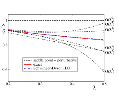
Figure 1: Comparison of perturbative (dashed lines), Schwinger-Dyson (dashed-dotted line) and exact, numerical evaluation of the two-point correlation (solid line) for the action with a unique classical vacuum ($\epsilon=1$). On this scale the NLO SDE solution is indistinguishable from the exact result.

For $\epsilon=-1$, SD equations truncated at any finite order cannot reproduce the exact result. This is because vertices in the SDE’s generated from the master equation originate from expansion around $x=0$, which is a local maximum and a metastable sate in higher dimensions. For $\epsilon=-1$, $\langle x^{2}\rangle$ is still positive and as a function of $\lambda$ it is non-analytical at $\lambda=0$, where it has a pole, while the LO solution Eq. (12) is analytical and for $\lambda=0$ gives $\langle x^{2}\rangle_{LO}=-1$! The action has two minima and in the saddle point approximation the integral in Eq. (1) is approximated by a sum of gaussian fluctuations around each of them with the difference between the full action and gaussian approximation treated as perturbation. This leads to

$$\langle x^{2}\rangle=\frac{6}{\lambda}-1-\frac{1}{2}\lambda-\frac{2}{3}\lambda^{2}-\frac{11}{8}\lambda^{3}-\frac{34}{9}\lambda^{4}-\frac{619}{48}\lambda^{5}+O(\lambda^{6})$$ (17)

and is compared to the exact, numerical result in Fig. 2

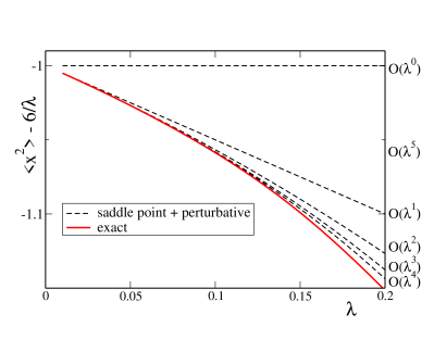
Figure 2: Saddle-point approximation computed to a varying order in $\lambda$ (dashed lines) compared with the exact result for $\epsilon=1$ obtained by numerical integration (solid line). The $O(\lambda^{4})$ perturbative results is indistinguishable form the exact result. For easier comparison we subtracted the leading, $6/\lambda$ term from $\langle x^{2}\rangle$. On this scale the solution of SD equation tends to $-6/\lambda\to-\infty$ as $\lambda\to 0$.

III Multiple quasi-degenerate vacua

In QCD large gauge transformations are not constrained by the Gauss’ law and result in topologically disconnected field configurations inst1 ; inst2 ; Reinhardt:1997rma ; Ford:1998bt ; Jahn:1998nw . In the semiclassical approximation these configurations correspond to degenerate classical vacua and the true vacuum state is a linear superposition of these vacua. To access the applicability of SDE equations in the case of such multiple saddle points, we again make a simple model for the action in $D=0+0$. Since there is no tunneling without the ”time” direction, it is possible that SDE’s equations in the realistic case with instantons are more accurate then the one ones in the no-time model discussed here.

To mimic the effect of multiple vacua in the partition function we consider the following action

$$S(x)=\frac{1}{g^{2}}\left[2(1-\cos(x))+\frac{x^{2}}{\Lambda^{2}}\right].$$ (18)

For simplicity, to be able to compare with SDE’s we define $x$ in the $(-\infty,+\infty)$ interval. The multiple saddle points originate from the $\cos$ term the role of the second term on rhs in Eq. 18 is to make the integral in Eq. (1) well defined. Because of this term the minima of $S(x)$ are not really degenerate, and their relative contribution depends on $\Lambda$. For weak coupling, $g<1$ the expectation value of $\langle x^{2}\rangle$ is determined in the saddle point approximation by the number of minima of the action. For fixed, finite $\Lambda$, $\langle x^{2}\rangle\to 0$ when $g\to 0$ since in this case the term $x^{2}/(g^{2}\Lambda^{2})$ is large for all minima of $\cos x$ except the one at $x=0$. In this limit, therefore, the integral becomes dominated by the single minimum at $x=0$ and one finds.

$$\langle x^{2}\rangle\to\frac{\Lambda^{2}g^{2}}{2(\Lambda^{2}+g^{2})}\to\frac{g^{2}}{2}.$$ (19)

Since the problem becomes effectively that of a single vacuum one expects the SDE to yield a similar result. This indeed is the case as shown in Fig. 4. As $\Lambda$ increases for fixed $g<1$ the contribution from the minima of $\cos x$ at $x=2\pi n$, $|n|>0$ are no longer suppressed and in the limit $\Lambda\to\infty$ one obtains

$$\langle x^{2}\rangle\to\frac{\Lambda^{2}}{2}.$$ (20)

This is an interesting limit, since even though there are multiple vacua contributing to the partition function integral their contribution is approximately equal to that of a broad minimum given by $x^{2}/\Lambda^{2}$ (c.f. Fig. 3), and it is this gaussian distribution that results in Eq. (20).

Figure 3: A typical action used here in a model study of multiple, quasi-degenerate vacua. For large $\Lambda$ and/or small $g$ the the number of minima contributing to the partition function is proportional to $\Lambda^{2}/g^{2}$. For the case shown in this figure, besides the central minimum there are additional $N=32$ local minima.

The SD equations for the action of Eq. (18) are derived from the operator identity

$$\frac{2}{g^{2}}\sin\left[-\frac{1}{\Gamma^{(2)}(y)}\frac{d}{dy}+y\right]+\frac{2y}{\Lambda^{2}}=-\Gamma^{(1)}(y).$$ (21)

In particular for the two-point correlation in the LO approximation, $\Gamma^{(2)}(y)=\Gamma^{(2)}_{0}$, it yields,

$$\frac{2}{g^{2}}\frac{d}{dy}\sin\left[-\frac{1}{\Gamma^{(2)}_{0}}\frac{d}{dy}+y\right]+\frac{2}{\Lambda^{2}}=-\Gamma^{(2)}_{0}.$$ (22)

The non-linear, algebraic equation for $\langle x^{2}\rangle=-1/\Gamma^{(2)}_{0}$ can be derived from the above by noticing that the argument of the sine can be written as an expectation value of ladder operators

$$\frac{d}{dy}\sin\left[-\frac{1}{\Gamma^{(2)}_{0}}\frac{d}{dy}+y\right]=\sqrt{\langle x^{2}\rangle}\langle 0|a\sin\left[\frac{a+a^{{\dagger}}}{\sqrt{\langle x^{2}\rangle}}\right]|0\rangle$$ (23)

with $a\equiv 1/\sqrt{\langle x^{2}\rangle}d/dy$ and $a^{{\dagger}}\equiv\sqrt{\langle x^{2}\rangle}y$. It finally leads to the following gap equation

$$\frac{2}{g^{2}}e^{-\frac{\langle x^{2}\rangle}{2}}+\frac{2}{\Lambda^{2}}=\frac{1}{\langle x^{2}\rangle}.$$ (24)

It can be verified that for finite $\Lambda$ in the $g\to 0$ limit the solution of Eq. (24) agrees with Eq. (19) while in the limit $\Lambda\to\infty$ it agrees with Eq. (20) In the former case, as discussed above, the SD equation reproduces the result of the problem with a unique vacuum. For large-$\Lambda$ on the other hand, it indeed follows from Eq. (24) that even though multiple saddle points contribute the net effect is equivalent to that of a single minimum with a large width $\sim\Lambda$ leading to solution for $\langle x^{2}\rangle$ that agrees with Eq. (20), as shown in Fig. 4.

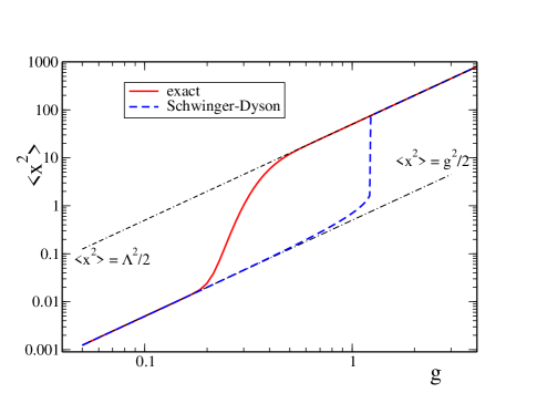
Figure 4: Comparison between exact (solid line) and Schwinger-Dyson, Eq. (24) approximation (dashed line) to $\langle x^{2}\rangle$ for the action given by Eq. (18). We used $g^{2}/\Lambda^{2}=0.01$ (cf. Fig.3). The dashed-dotted lines correspond to the two limits given by Eqs. (19), (20), were, as discussed in the text Schwinger-Dyson approximation becomes exact. For the range of couplings shown the saddle point approximation of Eq. (25) is indistinguishable from the exact result and involves summation over $N=33$ saddle points.

Outside of the two limits, several local minima of he action contribute to the partition function and the LO SD equation fails. This is seen in Fig. 4 for $g$ in the mid-range, $0.2\mathrel{\hbox to0.0pt{\lower 4.0pt\hbox{\hskip 1.0pt$\sim$}\hss}\raise 1.0pt\hbox{$<$}}g\mathrel{\hbox to0.0pt{\lower 4.0pt\hbox{\hskip 1.0pt$\sim$}\hss}\raise 1.0pt\hbox{$<$}}1$. In this range, where multiple minima contribute one expects summing over integrals around all saddle points is a better approximation to the generating functional compared to the SDE. In this, saddle point approximation

$$\langle x^{2}\rangle=\frac{\sum_{i=1}^{N}(x_{i}^{2}+\frac{1}{2\omega_{i}})\frac{e^{-S(x_{i})}}{\sqrt{\omega_{i}}}}{\sum_{i=1}^{N}\frac{e^{-S(x_{i})}}{\sqrt{\omega_{i}}}}$$ (25)

and comparison with the exact, numerical result is shown in Fig. 5. Indeed the saddle point approximation works while SDE fails in this range of couplings.

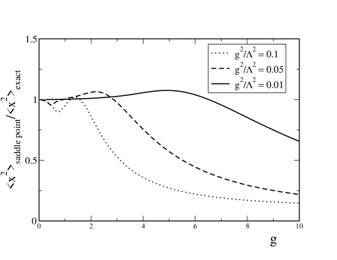
Figure 5: Comparison between exact, numerical computation and the saddle point approximation to $\langle x^{2}\rangle$ for different values of $g^{2}/\Lambda^{2}$. As $\Lambda$ increases for fixed $g$ so does the number of saddle points. The three cases shown correspond to $N=3,7,33$ points respectively (cf. Eq. (25)). As $\Lambda$ increases, saddle points become degenerate and Eq. 25 becomes an increasingly better approximation.

IV Particle on a circle

In QCD the domain of gauge fixed gluon field, i.e. the fundamental modular region may be non-flat with a non-trivial measure specified by the Fadeev-Popov determinant Gribov:1977wm . This highly complicates the Schwinger-Dyson formalism, which needs to take into account the boundary of fundamental modular region or the Gribov horizon Zwanziger:1989mf . In the following example we investigate what happens in a model in which the dynamical variable has a non-trivial boundary under an approximation when this boundary is ignored. For this purpose we consider quantum mechanics of a particle on a circle poc i.e. $D=0+1$ dimensional field theory. The variable $x(t)$ now describes location of the particle on a unit circle $0\leq x(t)<2\pi$ as a function of time and for the Hamiltonian we choose the free kinetic energy for a particle of unit mass $2H=p^{2}=-\partial^{2}_{x}$. Since the manifold is compact, the wave function must satisfy the boundary condition $\psi(x)=\exp(i\theta)\psi(x+2\pi)$ and in the following we take $\theta=0$. The normalized eigenvectors of the Hamiltonian are spanned by $\psi_{m}(x)=\exp(imx)/\sqrt{2\pi}$ with integer $m$ and the corresponding energies are $E_{m}=m^{2}/2$. The vacuum expectation value at the euclidean time ($t=-i\beta$), i.e. temperature-dependent correlation function is then given by

$$\langle x(\beta)x(0)\rangle=\langle 0|xe^{-\beta H}x|0\rangle=\pi^{2}+\sum_{m\neq 0}\frac{e^{-\beta\frac{m^{2}}{2}}}{m^{2}}.$$ (26)

At low temperatures, $T=1/\beta\to 0$ the correlation function is dominated by the lowest energy quantum sate and $\langle x(\infty)x(0)\rangle\to\pi^{2}$. In this case the restriction that $x$ be on a circle is important. At high temperatures, however, the system becomes semiclassical, and the particulars of the topology of the quantum system should become irrelevant. Also in this limit expectation values should be well approximated by contributions from small amplitude fluctuations around solutions of the classical equation of motion. In this case truncated SD equations should also be a good approximation. In our simple example we assume no interaction thus the SD equation and the semiclassical, saddle point approximation give the same results and both of them pertain to a formulation of the problem in terms of the variable dual to quantum number $m$  Banks:1977cc . This variable is just is the classical coordinate $x$ and the duality transformation $m\leftrightarrow x$ is given by

$$e^{-\beta\frac{m^{2}}{2}}=\int_{-\infty}^{\infty}\frac{dx}{\sqrt{2\pi\beta}}e^{-\frac{x^{2}}{2\beta}-imx}$$ (27)

leading to

$$\langle x(\beta)x(0)\rangle=\int_{0}^{2\pi}\frac{dx^{\prime}}{2\pi}\frac{dx}{2\pi}x^{\prime}\langle x^{\prime},\beta|x,0\rangle x$$ (28)

where

$$\langle x^{\prime},\beta|x,0\rangle=\sqrt{\frac{2\pi}{\beta}}\sum_{q\in N}\exp\left(-\frac{(x^{\prime}-x+2\pi q)^{2}}{2\beta}\right).$$ (29)

At finite temperature, $q$ counts the number of times the particle wraps around the circle. The duality between $m$ and $x$ is clear; at high temperature, $\beta\to 0$ and $x$ is well defined, (while $m$ is not) since

$$\langle x^{\prime},\beta|x,0\rangle\to 2\pi\delta(x^{\prime}-x)$$ (30)

with only the term with $q=0$ contributing. It then immediately follows that, $\langle x(0)x(0)\rangle=4\pi^{2}/3$. In the high temperature limit, the quantum variable $m$ is not well defined, i.e. in the sum in Eq. (26) an infinite number of terms contribute to give $4\pi^{2}/3$. At low temperatures, on the other hand, the system is quantum. As $\beta\to\infty$, $m$ becomes well defined, $m\to 0$ (while $x$ is not) and $\langle x(\infty)x(0)\rangle\to\pi^{2}$. To obtain the low temperature limit of the correlation function using the classical representation of Eq. (29) it is necessary to integrate over the entire range of $x$ and $x^{\prime}$. Furthermore it is necessary to allow $x$ (or $x^{\prime}$) to wrap around the circle an arbitrary number of times i.e. sum over all $q\in N$. The approximation in which the topology of the boundary is ignored corresponds to retaining only the $q=0$ term in the sum in Eq. (29), which, as follows from the discussion above, should work fine in the high temperature limit but fail at low temperatures. This is shown in Fig. 6.

V Summary

Phenomenological applications of Schwinger-Dyson equations require truncations in the number of retained effective interactions. It is important to access the reliability of such truncation in QCD where Green’s functions are not necessarily dominated by small fluctuations around the perturbative vacuum. In particular, confinement is expected to be related to topologically non-trivial field configuraiton like magnetic monoples and vortices that lie on the Gribov horizon Greensite:2004ke and produce tunneling between the degenerate, local minima of the action. If the effective potential for gauge degrees of freedom were known in principle one could compare the SDE approach with other, i.e. semiclassical approximations, (as can be done for example in the case of compact QED Drell:1978hr ). Here we have done such comparison in simple models to illustrate strengths and potential limitations of the SDE approach. In particular we have shown that if the partition function integral is dominated by a single semiclassical configuration, (one saddle point of the action), even the one-loop SD equation gives a much better approximation for a two-point correlation than perturbative series truncated at some high order. In the case of multiple-saddle points, however, we have shown that the semiclassical approximation, when applicable is more reliable while the SDE approach may not necessarily be capturing the correct physics. In such cases SDE’s can, however be successful when formulated in dual variables. Clearly the models studied here are very naive and more realistic problems need to be considered before definite conclusions about applicability of truncated SD equations to describe physics of confinement are made.

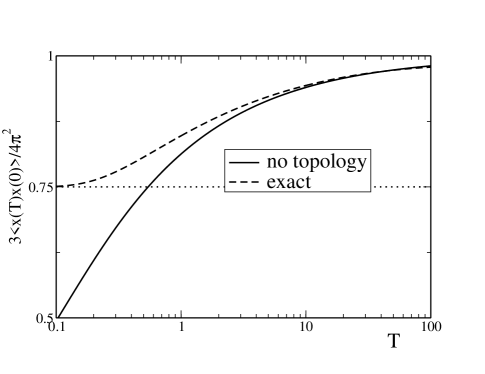
Figure 6: Comparison between exact (dashed line) and approximate evaluation of the correlation function as a function of temperature. In the approximation Eq. (29) only the $q=0$ term is retained.

- (1) C. D. Roberts and A. G. Williams, Prog. Part. Nucl. Phys. 33, 477 (1994).
- (2) R. Alkofer and L. von Smekal, Phys. Rept. 353, 281 (2001).
- (3) P. Maris and C. D. Roberts, Int. J. Mod. Phys. E 12, 297 (2003).
- (4) R. Alkofer, C. S. Fischer and F. J. Llanes-Estrada, Phys. Lett. B 611, 279 (2005) [Erratum-ibid. 670, 460 (2009)].
- (5) R. Alkofer, C. S. Fischer, F. J. Llanes-Estrada and K. Schwenzer, Annals Phys. 324, 106 (2009).
- (6) L. Del Debbio, M. Faber, J. Greensite and S. Olejnik, Phys. Rev. D 55, 2298 (1997).
- (7) K. Langfeld, H. Reinhardt and O. Tennert, Phys. Lett. B 419, 317 (1998).
- (8) M. Engelhardt, K. Langfeld, H. Reinhardt and O. Tennert, Phys. Rev. D 61, 054504 (2000).
- (9) J. Greensite, Prog. Part. Nucl. Phys. 51, 1 (2003).
- (10) Y. Nambu, Phys. Rev. D 10, 4262 (1974).
- (11) S. Mandelstam, Phys. Lett. B 53, 476 (1975).
- (12) A. M. Polyakov, Nucl. Phys. B 120, 429 (1977).
- (13) G. ’t Hooft, Nucl. Phys. B 190, 455 (1981).
- (14) L. von Smekal, A. Hauck and R. Alkofer, Annals Phys. 267, 1 (1998) [Erratum-ibid. 269, 182 (1998)].
- (15) C. S. Fischer, A. Maas and J. M. Pawlowski, Annals Phys. 324, 2408 (2009).
- (16) A. C. Aguilar, D. Binosi and J. Papavassiliou, Phys. Rev. D 78, 025010 (2008).
- (17) J. M. Cornwall, Phys. Rev. D 57, 7589 (1998).
- (18) F. V. Gubarev, M. I. Polikarpov and V. I. Zakharov, Phys. Lett. B 438, 147 (1998).
- (19) M. N. Chernodub, M. I. Polikarpov and V. I. Zakharov, Phys. Lett. B 457, 147 (1999).
- (20) A. P. Szczepaniak and H. H. Matevosyan, Phys. Rev. D 81, 094007 (2010).
- (21) C. Adam, Czech. J. Phys. 46, 893 (1996).
- (22) T. Radozycki, Phys. Rev. D 60, 105027 (1999).
- (23) P. Orland, Nucl. Phys. B 428, 221 (1994).
- (24) M. Sato and S. Yahikozawa, Nucl. Phys. B 436, 100 (1995).
- (25) E. T. Akhmedov, M. N. Chernodub, M. I. Polikarpov and M. A. Zubkov, Phys. Rev. D 53, 2087 (1996).
- (26) M. I. Polikarpov, U. J. Wiese and M. A. Zubkov, Phys. Lett. B 309, 133 (1993).
- (27) R. Jackiw and C. Rebbi, Phys. Rev. Lett. 37, 172 (1976).
- (28) A. Belavin, A. Polyakov, A. Schwartz, and Yu. Tyupkin, Phys. Lett. 59, 85 (1975).
- (29) H. Reinhardt, Nucl. Phys. B 503 (1997) 505.
- (30) C. Ford, U. G. Mitreuter, T. Tok, A. Wipf, J. M. Pawlowski, Annals Phys. 269, 26-50 (1998).
- (31) O. Jahn, F. Lenz, Phys. Rev. D58, 085006 (1998).
- (32) V. N. Gribov, Nucl. Phys. B 139, 1 (1978).
- (33) D. Zwanziger, Nucl. Phys. B 323, 513 (1989).
- (34) N. Fjeldso, J, Midtdal, and F. Ravndal, J. Phys. A: Math. Gen. 21, 1633 (1988).
- (35) T. Banks, R. Myerson and J. B. Kogut, Nucl. Phys. B 129, 493 (1977).
- (36) S. D. Drell, H. R. Quinn, B. Svetitsky and M. Weinstein, Phys. Rev. D 19, 619 (1979).
- (37) J. Greensite, S. Olejnik, D. Zwanziger, Phys. Rev. D69, 074506 (2004).