Almost classical solutions to the total variation flow

Instytut Matematyki Stosowanej i Mechaniki, Uniwersytet Warszawski
ul. Banacha 2, 02-097 Warszawa, Poland
E-mail: p.mucha@mimuw.edu.pl, p.rybka@mimuw.edu.pl

Abstract. The paper examines one-dimensional total variation flow equation with Dirichlet boundary conditions. Thanks to a new concept of “almost classical” solutions we are able to determine evolution of facets – flat regions of solutions. A key element of our approach is the natural regularity determined by nonlinear elliptic operator, for which $x^{2}$ is an irregular function. Such a point of view allows us to construct solutions. We apply this idea to implement our approach to numerical simulations for typical initial data. Due to the nature of Dirichlet data any monotone function is an equilibrium. We prove that each solution reaches such steady state in a finite time.

MSC: 35K55, 35K67, 74N05, 94A08.

Key words: total variation flow, optimal regularity, structure of solutions, almost classical solutions, sudden directional diffusion.

1 Introduction

The equation which is the topic of this paper

$$u_{t}-\frac{d}{dx}\left(\hbox{\rm sgn}\,(u_{x})\right)=0,\qquad u(a)=a_{b},\quad u(b)=a_{e}.$$ (1.1)

is a one-dimensional example of the total-variation flow. The motivation to study this problem is twofold: a) image analysis, see [ROF], [AC1], [Al]; b) crystal growth problems, see [AG], [Ta], [GGK], [Ma]. There are different physically relevant models, where a similar to ours surface energy appears, but the corresponding evolutionary problem is not necessarily set up, see e.g. [BL].

Equation (1.1) may be interpreted as a steepest descent of the total variation, i.e. we can write (1.1) as a gradient flow $u_{t}\in-\partial E(u)$ for a functional $E$. This is why we can apply the abstract nonlinear semigroup theory of Komura, see [Br], [Ba], to obtain existence of solutions. This has been performed by [FG], [KG], [GGK] and also by [ABC], [ABa], [ACD], [BCN]. However, the generality of this tool does not permit to study fine points of solutions to (1.1).

Solutions to (1.1) enjoy interesting properties, Fukui and Giga, [FG], have noticed that facets persist. By a facet we mean a flat part (i.e. affine) of the solution with zero slope. Zero is exactly the point of singularity of function $|\cdot|$. This is why the problem of facet evolution is not only nonlocal but highly anisotropic. Our equation (1.1) is at least formally parabolic of the second order. This is why we call the above behavior of solutions the sudden directional diffusion. However, even more dramatic effects of singular diffussion can be seen in the fourth order problems, see [GG]

As we have already mentioned some properties of facets were established in [FG], e.g. their finite speed of propagation was calculated. What is missing is the description of the process how they merge and how they are created. In [MR2] we studied a problem similar to (1.1). We worked there with a simplification of the flow of a closed curve by the singular mean weighted curvature. We have shown existence of so-called almost classical solutions, i.e. there is a finite number of time instances when the time derivative does not exist. However the results of [MR2] indicate lack of efficiency of the methods used there. This fact is our motivation to rebuilt the theory from the very beginning. For this reason we consider here the model system admitting effects of sudden directional diffusion. Hoping that our approach will be suitable for more general systems.

Our approach is as follows. We notice that the implicit time discretization leads to a series of Yosida approximations to the operator on the right-hand-side (r.h.s. for short) of (1.1). We study them quite precisely, because we consider variable time steps. As a result we capture the moment when two facets merge. We do not perform any further special considerations. We want to see how the regularity of original solutions is transported via solvability of the Yosida approximation. Due to the one-dimensional character of the problem we are able to obtain a result so good that it is of the maximal regularity character, what is rather expected for quasilinear parabolic systems. Let us underline that properly understood smoothness is the most important question connected to solvability of the original system. We have to modify standard regularity setting in order to capture all phenomena appearing in the system we study. As a result of our considerations we come to the conclusion that the best smoothness we could expect for a solution $u$ that $u(\cdot,t)$ be piecewise linear function, while $x^{2}$ is an example of an irregular function.

Our main goal is monitoring the evolution, as well creation, of the facets and a precise description of the regularity of solutions to (1.1), which we construct here. For this purpose we apply methods, which are distinctively different from those in the literature. We develop ideas which appeared in our earlier works. The key point is a construction of a proper composition of two multivalued operators: the first one is sgn  understood as a maximal monotone graph, the other one is $u_{x}$, which is defined only a.e. We leave aside the issue that in general this is a measure, not a function. This problem is resolved differently by the authors applying the semigroup approach, [FG], [AC1], [GGK], [BCN] etc. We treat $u_{x}$ as a Clarke differential (see (2.1) and the text below this formula). Here, we show that this composition is helpful when:
(a) we construct solutions, see Theorem 3.1;
(b) we discuss regularity of solutions, see Theorems 2.1 and 2.2.
At the moment, however, the usefulness of this approach is limited to one dimension. The advantage of our method is also simplicity, the composition is explicitly computable. As an extra result we obtain asymptotics of solutions. The Dirichlet boundary conditions imply that the set of possible equilibria consists of monotone functions. Our analysis shows that steady state must be reached in finite time.

On the other hand, there are two sorts of results available up to now to deal with (1.1):
1) the method based on the abstract semigroup theory, see e.g. [FG], [AC1], [GGK] and [BCN]. It is very general and elegant, it enables us to study the facet motion, but it does not capture all relevant information. The intrinsic difficulty associated with this method is the fact that the energy functional corresponding to (1.1) is not coercive, also see below Lemma 2.1 and the proof of Theorem 3.1.
2) the method based on the appropriate definition of the viscosity solution [TGO]. However, a different kind of problem was studied there. This is an active research field, see [GGR].

Our approach is based on the Yosida approximation, defined by as a solution of the resolvent problem

$$\lambda u-\frac{d}{dx}\left(\hbox{\rm sgn}\,(u_{x})\right)=\lambda v\qquad\hbox{in }(a,b),\quad(u-v)|_{\partial[a,b]}=0.$$ (1.2)

There are a couple of points to be made here. Firstly, we will construct $u$, a solution to (1.2), by very simple means, this is done is Section 3. This process resembles looking for a good notion of a weak solutions to a PDE. Since we came up with an integral equation we will call its solutions mild ones, see formula (3.16).

Secondly, (1.2) may be interpreted as an Euler-Lagrange equation for a non-standard variational functional. Namely, we set

$$\mathcal{J}(u)=\left\{\begin{array}[]{ll}\int_{a}^{b}|Du|&\hbox{if }u\in D(\mathcal{J})\equiv\{u\in BV[a,b],\ u(a)=a_{b},\ u(b)=a_{e}\},\\ +\infty&\hbox{if }L_{2}(a,b)\setminus D(\mathcal{J}),\end{array}\right.$$ (1.3)

where $\int_{a}^{b}|Du|$ is the total variation of measure $Du$. We stress that we consider the space $BV$ over a closed interval. Then, (1.2) may be seen as

$$v\in u+h\partial\mathcal{J}(u),$$ (1.4)

where $\partial\mathcal{J}$ is the subdifferential of $\mathcal{J}$ and $h=\frac{1}{\lambda}$. We shall see that the well-established convex analysis will yield existence of a unique solution to inclusion (1.4). This solution will be called variational. Since variational solutions are stronger (we shall see this), thus both solutions coincide.

We note that the Dirichlet problem in the multidimensional case is much more difficult, in particular the meaning of the boundary condition is not clear, see [AC2].

Thus, no matter which point of view we adopted, $u$ is given as the action of the nonlinear resolvent operator $R(\lambda,A)$ on $v$, i.e.

$$u=R(\lambda,A)(v)\equiv(\lambda+A)^{-1}(v),$$

where $A=-\frac{\partial}{\partial x}\hbox{\rm sgn}\,\frac{\partial}{\partial x}$. However, the notion of a mild solution to (1.2) does not permit us to interpret this equation easily. On the other hand, by convex analysis, we can see (1.2) as an inclusion (1.4).

The definition of the nonlinear resolvent operator leads to a detailed study of $\mathcal{J}$. One of our results, see Theorem 5.2 is a characterization of solutions to (1.2). The advantage of (1.2) is that it permits to monitor closely behavior of facets. It says that the regularity propagates. That is, if $v$ is such that $v_{x}$ belongs to the $BV$ space and the number of connected components of the properly understood set $\{x:v_{x}(x)=0\}$ is finite, then $u_{x}$ has the same property for sufficiently large $\lambda$.

It is well-known that the nonlinear resolvent leads to Yosida approximation, which is the key object in the construction of the nonlinear semigroup in the Komura theory. Namely, we set

$$A_{\lambda}u=\lambda(u-R(\lambda,A)(\lambda u)).$$ (1.5)

Our observation is that a maximal monotone multivalued operator like sgn  taking values in $[-1,1]$ may be composed with a multifunction properly generalizing a function of bounded total variation. We shall describe here this composition denoted by $\bar{\circ}$, see Section 2. We introduced such an operation in [MR2], see also [MR3]. We also point to an essential difficulty here, which is the problem of composition of two multivalued operators. Even if both of them are maximal monotone, the result need not be monotone nor single valued. If the outer of the two operators we compose is a subdifferential, then we expect that the result is closely related to the minimal section of the subdifferential.

One of our main results says that $A_{\lambda}u$ defined by (1.5) indeed converges to $-\frac{\partial}{\partial x}\hbox{\rm sgn}\,\bar{\circ}\,u_{x}$. Moreover, we have an error estimate, see Theorem 3.1, formula (3.4). In this way we justify correctness of the new notion. Due to the “explicit” nature of $\bar{\circ}$, we may better describe the regularity of solutions to (1.2).

Once we have constructed the Yosida approximation, we show existence of solution to the approximating problem $u^{\lambda}_{t}=-A_{\lambda}(u^{\lambda})$ on short time intervals, where $u^{\lambda}(t_{0})$ is given. This is done in Lemma 4.1. In fact, the method is close in spirit to the construction of the nonlinear semigroup, see [CL]. Convergence of the approximate solutions is shown at the end of Section 4. Here, we use the full power of the Yosida approximation to capture the finite number of time instances when the solution $u(t)$ is just right differentiable with respect to time, otherwise the derivative exists. The point is that we can control the distance to the original problem (1.1), so that we can monitor the time instances when facets merge.

Let us tell few words about the approach of proving our result. First, we define a space of admissible functions giving regularity of constructed solutions. Furthermore, we state main results together with an explanation of the meaning of almost classical solutions. In Section 3 we study the Yosida approximation for our system, concentrating on qualitative analysis of solutions. Proofs in this part are based on a direct construction which is possible due to the fine properties of chosen regularity. Subsequently, we prove the main results concerning existence and regularity. Section 5 is devoted to an alternative proof of existence for the resolvent operator based on the classical approach via Calculus of Variations. This analysis shows that restrictions taken in Sections 3 and 4 are natural and reasonable. Finally, we study the asymptotics of solutions and present an example of an explicit solution. We conclude our paper with numerical simulations. They are based upon the semidiscretization. Since they present a series of time snapshots, these pictures contain only the round-off error. At each time step there is no discretization error. The examples in Section 6 present the typical behavior, for which each solution becomes a monotone function in finite time.

2 The composition $\bar{\circ}\,$ and the main result

Our main goal is to present a new approach to solvability of systems of type (1.1). We construct a solution with this novel technique, and next we compare it with ones obtained in a more standard approach. This will clarify why some assumptions, which seem to be artificial, after deeper analysis will look completely natural. The total variation flow is a good example for such experiment, since we know precisely the solution, additionally its simple form allows us to deduce the qualitative properties by standard methods of the calculus of variation.

The first step is to define the basic regularity class of functions.

Definition 2.1.

(cf. [Z, Chapter 5]) We say that a real valued function $u$, defined over a closed interval $[a,b]$, belongs to $BV[a,b]$, provided that

$$\|Du\|\equiv\int_{a}^{b}|Du|<\infty,$$

where $|Du|$ is the total variation of the measure $Du$. We recall that

$$\|u\|_{BV[a,b]}=\|Du\|+\|u\|_{1}.$$

For the sake of definiteness, but without any loss of generality we assume that $[a,b]=[0,1]$.

Additionally, we treat $BV$ functions as multi-valued function. This is easy for functions which are derivatives, $u_{x}\in BV[a,b]$. This is very useful in the regularity study of solution to (1.1). Indeed, if $u$ and $u_{x}$ belong to $BV[a,b]$, then $u$ is Lipschitz continuous. Hence, $\frac{d^{+}u}{dx}$ and $\frac{d^{-}u}{dx}$ exist everywhere and they differ on at most countable set. Thus, we may set

$$\partial_{x}u(s)=\{\tau u_{x}^{-}+(1-\tau)u_{x}^{+}:\ \tau\in[0,1]\}.$$ (2.1)

Under our assumptions on $u$, the set $\partial_{x}u(x)$ is the Clarke differential of $u$ and equality holds in (2.1) due to [Cg, Section 2, Ex. 1]. If $u$ is convex, then $\partial_{x}u$ is the well-known subdifferential of $u$. As a result, if $u_{x}\in BV$, then for each $x_{0}\in(0,1)$, we have

$$\partial_{x}u(x_{0})=[\lim_{x\to x_{0}^{-}}u_{x}(x),\lim_{x\to x_{0}^{+}}u_{x}(x)]_{or},$$

where $[a,b]_{or}=[a,b]$ for $a\leq b$ and $[a,b]_{or}=[b,a]$ for $b>a$.

However, the description of solutions as functions whose derivatives belong to $BV$ is not sufficient. We have required to restrict our attention to its subclass. There is a need to control the facets, which we shall explain momentarily. A facet of $u$, $F$ is a closed, connected piece of graph of $u$ with zero slope, i.e. $F=F(\xi^{-},\xi^{+})=\{(x,y):\ y=const=u(x_{0}),\ x\in[\xi^{-},\xi^{+}]\}$, which is maximal with respect to inclusion of sets. The interval $[\xi^{-},\xi^{+}]$ will be called the set of parameters or preimage of facet $F$.

Let us recall that zero is the only point, where the absolute value, $|\cdot|$, the integrand in the definition of $\mathcal{J}$, fails to be differentiable. Thus, the special role of the zero slope and facets.

We shall also distinguish a subclass of facets. We shall say that a facet $F(\xi^{-},\xi^{+})$ has zero curvature, if and only if there is such $\epsilon>0$, that function $u$ restricted to $[\xi^{-}-\epsilon,\xi^{+}+\epsilon]$ is monotone. In the case the function under consideration is increasing this means that $u(\xi^{-}-\epsilon)<u(\xi^{-})=u(\xi^{+})<u(\xi^{+}+\epsilon)$. We shall see that zero curvature facets do not move at all. There may be even an infinite number of them. They have no influence on the evolution of the system. For that reason we introduce the following objects, capturing the essential phenomena. We shall say that a facet $F(\zeta^{-},\zeta^{+})$ of $u$ is an essential facet. It will be denoted by $F_{ess}(\zeta^{-},\zeta^{+})$, provided that there exists $\epsilon>0$ such that either

$u$ is decreasing on $(\zeta^{-}-\epsilon,\zeta^{-})$ and $u(t)>u(\zeta^{-})$ for $t\in(\zeta^{-}-\epsilon,\zeta^{-})$ and $u$ is increasing on $(\zeta^{+},\zeta^{+}+\epsilon)$ and $u(t)>u(\zeta^{+})$ for $t\in(\zeta^{+},\zeta^{+}+\epsilon)$ (then we call such a facet convex); moreover we set

$$\hbox{\rm sgn}\,\kappa_{[\zeta^{-},\zeta^{+}]}=1$$ (2.2)

or

$u$ is increasing on $(\zeta^{-}-\epsilon,\zeta^{-})$ and $u(t)<u(\zeta^{-})$ for $t\in(\zeta^{-}-\epsilon,\zeta^{-})$ and $u$ is decreasing on $(\zeta^{+},\zeta^{+}+\epsilon)$ and $u(t)<u(\zeta^{+})$ for $t\in(\zeta^{+},\zeta^{+}+\epsilon)$ (then we call such facet concave); moreover, we set

$$\hbox{\rm sgn}\,\kappa_{[\zeta^{-},\zeta^{+}]}=-1.$$ (2.3)

It may happen that $\zeta^{-}=\zeta^{+}=:\zeta$, then we shall call $F(\zeta,\zeta)$ a degenerate essential facet. In this case $u$ has a strict local minimum or a strict maximum at point $\zeta$.

We will call $\hbox{\rm sgn}\,\kappa_{[\zeta^{-},\zeta^{+}]}$ the transition number of facet $F(\zeta^{-},\zeta^{+})$. For the sake of consistency we set the transition number $\hbox{\rm sgn}\,\kappa_{[\zeta^{-},\zeta^{+}]}$ to zero for a zero curvature facet $F(\zeta^{-},\zeta^{+})$.

The union of parameter sets of all essential facets is denoted by $\Xi_{ess}(w)$ and $K_{ess}(w)$ is the number of essential facets, including degenerate facets.

Definition 2.2.

Let us suppose that $w=\partial_{x}u\in BV[0,1]$, where $u$ is absolutely continuous and $\partial_{x}u$ is the Clarke differential of $u$. We define $\Xi(w)=\{x\in[0,1]:0\in w(x)\}$. We say that $w$ as above is J-regular or shorter $w\in{\rm J}\mbox{-}{\rm R}$ iff the set $\Xi_{ess}(w)\subset\Xi(w)$ consists of a finite number of components, i.e.

$$\Xi_{ess}(w)=[a_{1},b_{1}]\cup\ldots\cup[a_{K_{ess}(w)},b_{K_{ess}(w)}]\quad\mbox{where }a_{i}\leq b_{i}$$ (2.4)

and each interval $[a^{i},b^{i}]$ is an argument set of an essential (nondegenerate or degenerate) facet $F(a^{i},b^{i})$. In particular, components of $\Xi(w)\setminus\Xi_{ess}(w)$ consists only of arguments of zero curvature facets of $u$.

Our definition in particular excludes functions with fast oscillations like $x^{2}\sin\frac{1}{x}$. We distinguished above a subset of $BV$ functions.

Since degenerate facets will be treated as pathology, for given $w\in{\rm J}\mbox{-}{\rm R}$, we define

$$L(w)=\min\{b-a:[a,b]\mbox{ is a connected component of }\Xi_{ess}(w)\}.$$ (2.5)

Note that $L(w)=0$ iff there exists a degenerate facet of $u$.

The name J-regular refers to the regularity of the integrand in the functional $\mathcal{J}$, which has singular point at $p=0$. $J$-regularity of $w=\partial u_{x}$ means that function $u$ can be split into finite number of subdomains where it is monotone.

We also define the following quantity,

$$\|w\|_{{\rm J}\mbox{-}{\rm R}[0,1]}=\|w\|_{BV[0,1]}+K_{ess}(w),$$ (2.6)

where $K_{ess}(w)$ is the number of connected parts of $\Xi_{ess}(w)$, however, this is not any norm in this space.

We start with the definition of a useful class of admissible functions.

Definition 2.3.

We shall say that a function $a$ is admissible, for short $a\in AF[0,1]$, iff $a:[0,1]\to\mathbb{R}$,

$$\alpha=\partial_{x}a\mbox{ ~{}~{}with~{}~{} }\alpha\in{\rm J}\mbox{-}{\rm R}\mbox{ ~{}~{}and~{}~{} }a(0)=a_{b},a(1)=a_{e}.$$ (2.7)

Here, $\partial_{x}a$ denotes the set-valued Clarke differential of $a$.

We note that the above definition restricts the behavior of admissible function at the boundary of the domain. Namely, if $a\in AF$, then $a$ is monotone on an interval $[0,x_{0})$ for some $x_{0}\in(0,1)$ and either

$$a(x_{0})>a(0)\mbox{~{}~{}~{} or~{}~{}~{} }a(x_{0})<a(0).$$

By the same token, $a$ is monotone on an interval $(x_{0},1]$ for some $x_{0}\in(0,1)$ and either

$$a(x_{0})>a(1)\mbox{~{}~{}~{} or~{}~{}~{} }a(x_{0})<a(1).$$

Thus, the Dirichlet boundary condition makes immobile any facet touching the boundary. Hence, such facets behave as if they had zero curvature.

A composition of multivalued operators requires proper preparations. Due to the needs of our paper, we restrict ourselves to a definition of

$$\hbox{\rm sgn}\,\bar{\circ}\,\alpha$$

for a suitable class of multivalued operators $\alpha$. Of course, it is most important to define this composition in the interior of the domain we work with. See also [MR2], [MR3].

Definition 2.4.

Let us suppose that $a$ is admissible and $\partial_{x}\beta=\alpha\in{\rm J}\mbox{-}{\rm R}[0,1]$. The definition of $\hbox{\rm sgn}\,\bar{\circ}\,\alpha$ is pointwise. Let us first consider $x\in[0,1]\setminus\Xi_{ess}(\alpha)$. Then, there exists an interval $(a,b)$ containing $x$ and such that either $\beta$ is increasing on $(a,b)$ or decreasing. In the first case we set

$$\hbox{\rm sgn}\,\bar{\circ}\,\alpha(x)=1;$$ (2.8)

if $\beta$ is decreasing on $(a,b)$, then we set

$$\hbox{\rm sgn}\,\bar{\circ}\,\alpha(x)=-1.$$ (2.9)

We note that the set $[0,1]\setminus\Xi_{ess}(\alpha)$ is a finite sum of open intervals, on each of them function $\beta$ is monotone. Furthermore, the end points of $[0,1]$ can not belong to $\Xi_{ess}(\alpha)$.

Now, let us consider $x\in\Xi_{ess}(\alpha)$, then there is $[p,q]$ a connected component of $\Xi_{ess}(\alpha)$ containing $x$. If $F(p,q)$ is a convex facet of $\beta$, then we set,

$$\hbox{\rm sgn}\,\bar{\circ}\,\alpha(x)=\frac{2}{q-p}x-\frac{2p}{q-p}-1\mbox{~{}~{}~{}~{}for~{}~{}}x\in[p,q].$$ (2.10)

If $F(p,q)$ is a concave facet of $\alpha$, then we set,

$$\hbox{\rm sgn}\,\bar{\circ}\,\alpha(x)=-\frac{2}{q-p}x+\frac{2p}{q-p}+1\mbox{~{}~{}~{}~{}for~{}~{}}x\in[p,q].$$ (2.11)

We have already mentioned that the Dirichlet boundary condition does not permit any motion of the facet touching the boundary. Thus, effectively, they behave like zero-curvature facets. Part 2 of Definition 2.4 takes this into account.

Now, we are in a position to state main results being also a justification of the notion of almost classical solutions to our system.

Theorem 2.1.

Let $u_{0}\in AF[0,1]$, $L(u_{0,x})>0$ with $u_{0}(0)=a_{b}$ and $u_{0}(1)=a_{e}$, then the system (1.1) admits unique solution in the sense specified by (3.16) and such that

$$u_{x}\in L_{\infty}(0,T;{\rm J}\mbox{-}{\rm R}[0,1]).$$ (2.12)

Moreover, $u$ is an almost classical solution, i.e. it fulfills (1.1) in the following sense

$$\begin{array}[]{lcr}u_{t}-\partial_{x}\hbox{\rm sgn}\,\bar{\circ}\,u_{x}=0&in&[0,1]\times(0,T),\\ u(0,t)=a_{b},\qquad u(1,t)=a_{e}&for&t\in[0,T),\\ u|_{t=0}=u_{0}&on&[0,1],\end{array}$$ (2.13)

where the time derivative in (2.13) exists for all time instances, except for at most a finite number of exceptions, the $x$ derivative exists for at most a finite number of exceptions. Additionally, $u(\cdot,t)\in AF[0,1]$ for $t\in[0,T]$.

We study a second order parabolic equation with the goal of establishing existence of almost classical solutions. This is why we do not consider general data in $L_{2}$, but those which are more natural for this problem, where the jumps in $u_{x}$ and their number matter most. This is why we look for $u$, which not only belongs to $BV$, i.e. $u(\cdot,t)\in BV$, but also $u(\cdot,t)\in AF$. In addition, the necessity of introducing essential facets will be explained.

An improvement of the above result, showing a regularization effects, is the following

Theorem 2.2.

Let $u_{0}$ be as in previous Theorem above, but $L(u_{0,x})=0$. Then, there exists a unique mild solution to (1.1), which is almost classical and it fulfills (2.13). Furthermore, $L(u_{x}(t))>0$ for $t>0$.

The second theorem shows that the class of functions with non-degenerate facets is typical, and each initially degenerate essential facet momentarily evolve into an nontrivial interval. Furthermore, creation of such a singularity is impossible. In order to explain this phenomena let us analyze the following very important example related to analysis of nonlinear elliptic operator defined by subdifferential of (1.3).

We first recall the basic definition. We say that $w\in\partial\mathcal{J}(u)$ iff $w\in L_{2}(a,b)$ and for all $h\in L_{2}(a,b)$ the inequality holds,

$$\mathcal{J}(u+h)-\mathcal{J}(u)\geq(w,h)_{2}.$$ (2.14)

Here $(f,g)_{2}$ stands for the regular inner product in $L_{2}(a,b)$. We also say that $v\in D(\partial\mathcal{J})$, i.e. $v$ belongs to the domain of $\partial\mathcal{J}$ iff $\partial\mathcal{J}(v)\neq\emptyset$.

We state here our fundamental example. We recall (1.3) and for the sake of convenience we set $(a,b)=(-1,1)$. Then we make the following observation.

Lemma 2.1.

Function $\frac{1}{2}x^{2}$ does not belong to $D(\partial\mathcal{J})$.

Proof. If $\frac{1}{2}x^{2}\in D(\partial\mathcal{J})$, then there existed $w\in L_{2}(-1,1)$ such that for all $\phi\in C^{\infty}_{0}(-1,1)$ and $t\in\mathbb{R}$

$$\int_{(-1,1)}(|x+t\phi_{x}|-|x|)dx\geq t\int_{(-1,1)}w\phi dx.$$ (2.15)

We restrict ourselves to $\phi$ such that

$$\phi\in C^{\infty}_{0}(-\delta,\delta)\mbox{~{}~{}~{}~{} and ~{}~{}~{}~{} supp}\,\phi_{x}[-\delta,-\delta/2]\cup[\delta/2,\delta].$$

Additionally,

$$\phi_{x}(t)>0\mbox{ ~{} for ~{} }t\in(-\delta,-\delta/2),\phi_{x}(t)<0\mbox{ ~{} for ~{} }t\in(\delta/2,-\delta)$$

and

$$\phi(-\delta)=\phi(\delta)=0,\phi(t)=1\mbox{ ~{} for ~{}}t\in(-\delta/2,\delta/2).$$

Next, let us observe that

$$|x+t\phi_{x}(x)|-|x|=t\phi_{x}(x)\hbox{\rm sgn}\,x\mbox{ ~{}~{}~{} for ~{}}|t\phi_{x}(x)|\leq\delta/2;$$ (2.16)

we keep in mind that $\phi_{x}(t)=0$ for $t\in(-\delta/2,\delta/2)$.

Thus, for such $\phi$ and $t$ the r.h.s. of (2.15) equals

$$\int_{(-\delta/2,\delta/2)}(|x+t\phi_{x}(x)|-|x|)dx=\int_{(-\delta,-\delta/2)}t\phi_{x}\cdot(-1)dx+\int_{(\delta/2,\delta)}t\phi_{x}\cdot(1)dx=-2t.$$ (2.17)

Hence, we get

$$-2t\geq t\int_{(-\delta,\delta)}w\phi dx,$$

what implies for $t>0$

$$2\leq-\int_{(-\delta,\delta)}w\phi dx\leq\int_{(-\delta,\delta)}|w|dx\to 0,$$ (2.18)

since $w\in L_{2}(-1,1)$. Thus, we have just reached a contradiction. Hence, $\frac{1}{2}x^{2}$ can not belong to $D(\partial\mathcal{J})$. ∎

The full description of the domain of the subdifferential $\partial\mathcal{J}$ of (1.3) is beyond the scope of this paper. There is a description of $D(\mathcal{J})$ for the multidimensional version of the problem we consider, see e.g. [AC2]. It is based on Anzellotti’s formula for integration by parts [Az]. However, a direct characterization of this set for the one-dimensional problem seems to be missing even though this functional has been studied in the literature.

At the end we mention a result describing the asymptotics of solutions, proved in the last section.

Theorem 2.3.

There is finite $t_{ext}>0$ such that the solution $u$ reaches a steady state at $t_{ext}$, i.e. $u(t)=u(t_{ext})$ for $t>t_{ext}$. Moreover, we have an explicit estimate for $t_{ext}$ in terms of $u_{0}$, see (6.1).

The above result shows that the limit of any solution, as time goes to infinity, is always a monotone function, and this will be proved and illustrated in Section 6. There we present numerical simulations based on the analysis of system (1.1). It is interesting to note that in comparison with [FOP] who deals with the multidimensional case, our computations do not contain any discretization error. A rich possibility of stationary states are allowed thanks to Dirichlet boundary conditions. Note that such picture is impossible for Neumann boundary constraints, for which there are only trivial/constant equilibria.

3 Yosida approximation

The central object for our considerations is the Yosida approximation to $-\partial_{x}\hbox{\rm sgn}\,\partial_{x}$. First, we introduce an auxiliary notion of a nonlinear resolvent operator to the following problem,

$$\lambda u-\frac{d}{dx}\hbox{\rm sgn}\,(u_{x})=\lambda v\mbox{ ~{}~{}~{} on ~{}~{} }[0,1],\qquad u=v\quad\hbox{ at }\partial[0,1],$$ (3.1)

where $v$ is a given element of $L_{2}(0,1)$.

Definition 3.1.

An operator assigning to $v\in{\rm J}\mbox{-}{\rm R}$ a unique solution, $u\in{\rm J}\mbox{-}{\rm R}$, to (3.1) will be called the resolvent of $A=-\partial_{x}\hbox{\rm sgn}\,\partial_{x}$ and we denote it by

$$u=R(\lambda,A)v.$$

Now, we may introduce the Yosida approximation to $A$.

Definition 3.2.

Let us assume that $A=-\partial_{x}\hbox{\rm sgn}\,\partial_{x}$ is as above and $\lambda>0$. An operator $A_{\lambda}:{\rm J}\mbox{-}{\rm R}\to{\rm J}\mbox{-}{\rm R}$ given by

$$A_{\lambda}u=\lambda(u-R(\lambda,A)(\lambda u))$$

is called the Yosida approximation of $A$.

Since the notion of Yosida approximation seems well-understood, we will use it to explain the meaning of $A$. For this purpose we will fix $w\in{\rm J}\mbox{-}{\rm R}$ and $\lambda>0$. We set $u^{\lambda}:=R(\lambda,A)w$. We will look more closely at $A_{\lambda}(u^{\lambda})$.

Theorem 3.1.

Let us assume that $w\in AF[0,1]$, i.e. $w_{x}\in{\rm J}\mbox{-}{\rm R}$, then there exists a unique solution to

$$\lambda u+A(u)=\lambda w\quad\hbox{in }(0,1),\qquad u(0)=w(0),\ u(1)=w(1),$$ (3.2)

denoted by $u^{\lambda}$, fulfilling

$$\|u^{\lambda}_{x}\|_{BV[0,1]}\leq\|w_{x}\|_{BV[0,1]}.$$ (3.3)

Moreover, there is $\lambda_{0}>0$ such that

$$K_{ess}(u^{\lambda}_{x})=K_{ess}(w_{x})\mbox{~{}~{}~{}~{}~{} for ~{}~{}}\lambda>\lambda_{0}\mbox{ ~{}~{} with ~{}~{} }\|u^{\lambda}_{x}\|_{{\rm J}\mbox{-}{\rm R}}\leq\|w_{x}\|_{{\rm J}\mbox{-}{\rm R}}.$$

Furthermore, if $L(w_{x})=d>0$, equation (3.2) can be restated as follows

$$\lambda u^{\lambda}-\partial_{x}\hbox{\rm sgn}\,\bar{\circ}u^{\lambda}_{x}=\lambda w+V(\lambda,x),$$ (3.4)

where $V(\lambda,x)\to 0$ in $L_{q}$ for all $q<\infty$ as $\lambda\to\infty$. In addition

$$A_{\lambda}(u^{\lambda})\to-\partial_{x}\hbox{\rm sgn}\,\bar{\circ}w_{x}\mbox{ ~{}~{}~{} in ~{}~{}~{} }L_{q}(0,1)\mbox{~{}~{}~{}with~{}~{}~{}}q<\infty.$$

Proof. We would like to present an independent proof of existence of solutions to system (3.2), which is based on simple tools, without any explicit reference to calculus of variations. For this purpose, we restrict ourselves to $w\in AF$ and for sufficiently large $\lambda$. A simple construction of $u^{\lambda}$ for a given $w$ based upon Lemma 3.1, is presented below.

Our assumptions give us

$$\Xi_{ess}(w_{x})=\bigcup_{i=1}^{K_{ess}(w_{x})}[a^{i}_{*},b^{i}_{*}]$$ (3.5)

with $a^{i}_{*}\leq b^{i}_{*}$. Moreover, $a^{1}_{*}>0$ and $b_{*}^{K_{ess}(w_{x})}<1$.

Below, we present a construction of $u^{\lambda}$. Namely, we consider system (3.2) in a neighborhood of preimage of an essential facet $[a^{i}_{*},b^{i}_{*}]$ of $w$ (it may be degenerate) and we prescribe the evolution of this facet. If $\lambda$ is sufficiently large, then we keep the number $K_{ess}$ constant.

Lemma 3.1.

Let us suppose that $w$ satisfies the assumptions of Theorem 3.1. Then, for sufficiently large $\lambda$, and for each $i=1,\ldots,K_{ess}(w_{x})$ there exist monotone functions

$$\lambda\mapsto a_{i}(\lambda)\quad\hbox{ and }\quad\lambda\mapsto b_{i}(\lambda),$$

which are solutions to the following problem,

$$(b^{i}(\lambda)-a^{i}(\lambda))w(a^{i}(\lambda))=\int_{a^{i}(\lambda)}^{b^{i}(\lambda)}w+2\frac{1}{\lambda}\hbox{\rm sgn}\,\kappa_{[a^{i}_{*},b^{i}_{*}]},\qquad w(b^{i}(\lambda))=w(a^{i}(\lambda)).$$ (3.6)

These solutions are defined locally, i.e. in a neighborhood of $[a^{i}_{*},b^{i}_{*}]$.

We recall that, the transition numbers $\hbox{\rm sgn}\,\kappa_{[a^{i}_{*},b^{i}_{*}]}$ were defined in (2.2), (2.3). Additionally, we require

$$a^{1}(\lambda)>0,\qquad b^{K_{ess}(w_{x})}(\lambda)<1\mbox{~{}~{} and~{}~{} }b^{i}(\lambda)<a^{i+1}(\lambda)\quad\hbox{for }i=1,\ldots,K_{ess}(w_{x})-1.$$ (3.7)

However, if $\lambda_{0}$ is the greatest lower bound of $\lambda$ as above, then one of the three possibilities occurs,

$$a^{1}(\lambda_{0})=0\quad\mbox{or}\quad b^{K(w_{x})}(\lambda_{0})=1\quad\mbox{or}\quad a^{i}(\lambda_{0})=b^{i+1}(\lambda_{0}).$$ (3.8)

It is worthwhile to underline that the lemma holds if $L(w_{x})=0$, too.

Proof. Let fix $i$ in $\{1,\ldots,K_{ess}(w_{x})\}$. Problem (3.6) comes from integration of equation (3.2) over a neighborhood of facet $[a^{i}_{*},b^{i}_{*}]$. For $\tau\in\mathbb{R}$ in a neighborhood of zero and such that $\tau\hbox{\rm sgn}\,\kappa_{[a_{*}^{i},b_{*}^{i}]}>0$, we set

$$\bar{a}^{i}(\tau)=\min(w|_{[b^{i-1}_{*},a^{i}_{*}]})^{-1}(w(a_{*}^{i})+\tau),\qquad\bar{b}^{i}(\tau)=\max(w|_{[b^{i}_{*},a^{i+1}_{*}]})^{-1}(w(b_{*}^{i})+\tau).$$ (3.9)

This definition is correct, because functions $w|_{[b^{i-1}_{*},a^{i}_{*}]}$ and $w|_{[b^{i}_{*},a^{i+1}_{*}]}$ are monotone. If these functions are strictly monotone, then $w^{-1}(w(b_{*}^{i})+\tau)$ is strictly monotone too, so the min/max are redundant. However, if there exists $\{\alpha\}\neq[\alpha,\beta]\subset\Xi(w)$ and $[\alpha,\beta]\subset[b^{i-1}_{*},a^{i}_{*}]$ (resp. $[\alpha,\beta]\subset[b^{i}_{*},a^{i+1}_{*}]$, then $(w|_{[b^{i-1}_{*},a^{i}_{*}]})^{-1}$ (resp. $(w|_{[b^{i}_{*},a^{i+1}_{*}]})^{-1}$) is a maximal monotone graph and min/max makes $\bar{a}^{i}(\cdot)$ (resp. $\bar{b}^{i}(\cdot)$) single valued and discontinuous. However, the function

$$\tau\mapsto(\bar{b}^{i}(\tau)-\bar{a}^{i}(\tau))w(\bar{a}^{i}(\tau))-\int_{\bar{a}^{i}(\tau)}^{\bar{b}^{i}(\tau)}w(s)\,ds=:F_{i}(\tau),\qquad i=1,\ldots,K_{ess}(w_{x}),$$

is continuous. Indeed, if $\tau_{0}$ is point, where $\bar{a}^{i}$ and $\bar{b}^{i}$ are continuous, then this statement is clear. Let us suppose that at $\tau_{0}$ function $\bar{a}^{i}$ has a jump (the argument for $\bar{b}^{i}$ is the same). Then, $[\bar{a}^{i}(\tau_{0}),\beta]\subset\Xi(w_{x})$, where $\bar{a}^{i}(\tau_{0})<\beta$ and for any $x\in[\bar{a}^{i}(\tau_{0}),\beta]$ we have

$$(\bar{b}^{i}(\tau_{0})-\bar{a}^{i}(\tau_{0}))w(\bar{a}^{i}(\tau_{0}))-\int_{\bar{a}^{i}(\tau_{0})}^{\bar{b}^{i}(\tau_{0})}w(s)\,ds=(\bar{b}^{i}(\tau_{0})-x)w(x)-\int_{x}^{\bar{b}^{i}(\tau)}w(s)\,ds.$$ (3.10)

This is so, because we notice that $w$ restricted to $[\bar{a}^{i}(\tau_{0}),\beta]$ is constant and equal to $w(a^{i}_{*})+\tau_{0}$. Moreover,

$$\int_{\bar{a}^{i}(\tau_{0})}^{\bar{b}^{i}(\tau_{0})}w(s)\,ds=\int_{\bar{a}^{i}(\tau_{0})}^{x}w(s)\,ds+\int_{x}^{\bar{b}^{i}(\tau_{0})}w(s)\,ds=(x-\bar{a}^{i}(\tau_{0}))(w(a^{i}_{*})+\tau_{0})+\int_{x}^{\bar{b}^{i}(\tau_{0})}w(s)\,ds.$$

Hence, our claim follows, i.e. continuity of $F_{i}$, $i=1,\ldots,K_{ess}(w)$. Indeed , let us suppose that $\tau_{n}$ converges from one side to $\tau_{0}$ (the side, left or right, depends upon $\hbox{\rm sgn}\,\kappa_{[a^{i}_{*},b^{i}_{*}]}$) so that $\lim_{n\to\infty}\bar{a}^{i}(\tau_{n})=\gamma$, where $\gamma=\bar{a}^{i}(\tau_{0})$ or $\gamma=\beta$. Then, due to (3.10) we deduce continuity of $F_{i}$.

Subsequently, if we take $\lambda$ sufficiently large, then $\frac{2}{\lambda}\hbox{\rm sgn}\,\kappa_{[a^{i}_{*},b^{i}_{*}]}$ is in the range of $F_{i}$, i.e. there exists $\tau_{i}=\tau_{i}(\lambda)$ such that $F_{i}(\tau(\lambda))=\frac{2}{\lambda}\hbox{\rm sgn}\,\kappa_{[a^{i}_{*},b^{i}_{*}]}$. If we further make $\lambda$ larger, then we can make sure that for each $i=1,\ldots,K_{ess}(w_{x})$ we have

$$\bar{b}^{i-1}(\tau_{i}(\lambda))<\bar{a}^{i}(\tau_{i}(\lambda))\quad\hbox{and}\quad\bar{b}^{i}(\tau_{i}(\lambda))<\bar{a}^{i+1}(\tau_{i}(\lambda)).$$

Thus, we set

$$a^{i}(\lambda):=\bar{a}^{i}(\tau_{i}(\lambda)),\qquad b^{i}(\lambda):=\bar{b}^{i}(\tau_{i}(\lambda)).$$

Let us define $\lambda_{0}$ to be the inf of $\lambda$’s constructed above.

We see that for $\lambda_{0}$ one of the inequalities

$$a^{1}(\lambda_{0})>0,\qquad b^{i}(\lambda_{0})<a^{i+1}(\lambda_{0}),\quad i=1,\ldots,K_{ess}(w_{x})-1,\qquad b^{K_{ess}(w_{x})}(\lambda_{0})<1.$$

become equality. $\Box$

This lemma permits us to define the function $u$ for $\lambda\geq\lambda_{0}$,

$$u^{\lambda}=\left\{\begin{array}[]{lcl}\displaystyle w&\mbox{for}&x\in[0,1]\setminus\bigcup_{i=1}^{K_{ess}(w_{x})}[a^{i}(\lambda),b^{i}(\lambda)]\\ \displaystyle w(a^{i})&\mbox{for}&x\in[a^{i}(\lambda),b^{i}(\lambda)]\end{array}\right.$$ (3.11)

We immediately notice that $K_{ess}(u^{\lambda}_{x})=K_{ess}(w_{x})$ and $\Xi_{ess}(u^{\lambda}_{x})=\bigcup_{i=1}^{K_{ess}(u^{\lambda}_{x})}[a^{i},b^{i}]$, provided that $\lambda>\lambda_{0}$.

Let us analyze what happens at $\lambda=\lambda_{0}$. We know that one of the three possibilities in (3.8) occurs. We notice that if $a^{1}(\lambda_{0})=0$ or $b^{K_{ess}(w_{x})}(\lambda_{0})=1$, then a facet of $u^{\lambda}$ touches the boundary. Subsequently this facet becomes a zero curvature facet, for it is immobile. This is a simple consequence of Dirichlet boundary conditions which do not admit any evolution of facets touching the boundary.

Let us look at the case $b^{i}(\lambda_{0})=a^{i+1}(\lambda_{0})$ for an index $i$. Thus, we obtain the phenomenon of facet merging. In both cases the structure of the set $\Xi_{ess}(u^{\lambda}_{x})$ will be different from $\Xi_{ess}(w_{x})$. As a result, we have

$$K_{ess}(u^{\lambda}_{x})<K_{ess}(w_{x}).$$ (3.12)

It is worth stressing that at the moment $\lambda=\lambda_{0}$ more than two facets may merge, so we can not control the decrease of number $K$. In this case we have to slightly modify (3.11), since the structure of $\Xi_{ess}(u^{\lambda}_{x})$ is different from $\Xi_{ess}(w_{x})$. It is sufficient to notice that the number of elements in the decomposition (3.5) has decreased.

It is clear that for $\lambda\geq\lambda_{0}$, we have

$$K_{ess}(u^{\lambda}_{x})\leq K_{ess}(w_{x})$$ (3.13)

and by the construction, (3.11) it is also obvious that (see Definition 2.1)

$$\|Du^{\lambda}_{x}\|\leq\|Dw_{x}\|.$$ (3.14)

Note that the boundary conditions are given, so (3.14) controls the whole norm of $u^{\lambda}$.

Once we constructed a solution $u^{\lambda}$ by (3.11), we shall discuss the question: in what sense does it satisfy equation (1.2). One hint is given in the process of construction $a^{i}(\lambda)$ and $b^{i}(\lambda)$. This is closely related to ideas in [MR1]. If we stick with differential inclusions, then formula

$$u-w-\frac{1}{\lambda}\frac{d}{dx}\hbox{\rm sgn}\,u_{x}\ni 0,$$ (3.15)

leads to difficulties, because we did not provide any definition of the last term on the left-hand-side (l.h.s. for short).

Here comes our meaning of a mild solution: for each $x\in[0,1]$, the following inclusion must hold

$$\int_{0}^{x}(u-w)dx^{\prime}-\left.\frac{1}{\lambda}\hbox{\rm sgn}\,u_{x}\right|_{0}^{x}\ni 0.$$ (3.16)

We shall keep in mind that at $x=0$, we have $u=w$ (for the sake of simplicity of notation we shall suppress the superscript $\lambda$, when this does not lead into confusion).

In order to show that $u$ fulfills (3.16), we will examine a neighborhood of the first component of $\Xi_{ess}(u_{x})$, i.e. $[a^{1},b^{1}]$. We take $x\in[0,a^{1})$, then $u=w$ on $[0,x]$. Thus, it is enough to check whether $\frac{1}{\lambda}(\hbox{\rm sgn}\,u_{x}(0)-\hbox{\rm sgn}\,u_{x}(x))\ni 0$. We notice that on $[0,x]\subset[0,a_{1})$ function $u$ is monotone. As a result $\hbox{\rm sgn}\,u_{x}(0)$ and $\hbox{\rm sgn}\,u_{x}(x)$ may equal $1$ or $[-1,1]$, provided that $u$ is increasing. If on the other hand, $u$ is decreasing on $[0,x]$, then $\hbox{\rm sgn}\,u_{x}(0)$ and $\hbox{\rm sgn}\,u_{x}(x)$ are equal to $-1$ or $[-1,1]$. If any of these possibilities occurs, then (3.16) is fulfilled.

We shall continue, after assuming for the sake of definiteness that facet $F(a^{1},b^{1})$ is convex. The argument for a concave facet is analogous.

Let us consider $x\in[a^{1},b^{1}]$. We interpret $\hbox{\rm sgn}\,t$ as a multivalued function such that $\hbox{\rm sgn}\,0=[-1,1]$. Then, we have for $x\in[a^{1},b^{1}]$

$$\int_{0}^{x}(u-w)dx^{\prime}-\frac{1}{\lambda}[-1,1]+\frac{1}{\lambda}\hbox{\rm sgn}\,u_{x}|_{x^{\prime}=0}\ni 0.$$ (3.17)

Since we assumed that the facet $F(a^{1},b^{1})$ is convex, from (3.6) we find that

$$0\leq\int_{0}^{x}(u-w)dx^{\prime}\leq\frac{2}{\lambda}.$$ (3.18)

By the assumption we know that $\hbox{\rm sgn}\,u_{x}|_{x^{\prime}=0}\ni-1$. Hence,

$$\int_{0}^{x}(u-w)dx^{\prime}-\frac{1}{\lambda}\in\frac{1}{\lambda}[-1,1].$$ (3.19)

This shows (3.16) again. In case $F(a^{1},b^{1})$ is concave, the argument is analogous.

Let us now consider $x\in(b^{1},a^{2}]$, then we have

$$\int_{0}^{x}(u-w)dx^{\prime}-\left.\frac{1}{\lambda}\hbox{\rm sgn}\,u_{x}\right|_{0}^{x} = \int_{0}^{a^{1}}(u-w)dx^{\prime}-\left.\frac{1}{\lambda}\hbox{\rm sgn}\,u_{x}\right|_{0}^{a^{1}}+\int_{a^{1}}^{b^{1}}(u-w)dx^{\prime}$$

$$-\left.\frac{1}{\lambda}\hbox{\rm sgn}\,u_{x}\right|_{a^{1}}^{b^{1}}+\int_{b^{1}}^{x}(u-w)dx^{\prime}-\left.\frac{1}{\lambda}\hbox{\rm sgn}\,u_{x}\right|_{b^{1}}^{x}$$

$$= I_{1}+I_{2}+I_{3}.$$

Here, we do have the freedom of choosing $\hbox{\rm sgn}\,u_{x}$ at $x=b^{1}$. Namely we set $\hbox{\rm sgn}\,u_{x}(b^{1})=-1$. We also know that $\hbox{\rm sgn}\,u_{x}(a^{1})=1$ .

We recall that by the very construction of $a^{1}$ and $b^{1}$, we have $I_{2}=0$. Subsequently, we notice that the argument performed for $x\in[0,a^{1})$ applies also to $x\in(b^{1},a^{2}]$, Thus,

$$I_{1}+I_{2}+I_{3} = -\frac{1}{\lambda}(1-\hbox{\rm sgn}\,u_{x}(0))+0-\frac{1}{\lambda}(-1+\hbox{\rm sgn}\,u_{x}(x))$$

$$= \frac{1}{\lambda}(-\hbox{\rm sgn}\,u_{x}(0)+\hbox{\rm sgn}\,u_{x}(x))\ni 0,$$

i.e. (3.16) holds again.

Repeating the above procedure for each subsequent facet, we prove that $u$ given by (3.13) fulfills (3.16). The case $x\in[b^{K_{ess}},1]$ is handled in the same way. Thus, we proved the first part of Theorem 3.1 concerning existence.

We shall look more closely at the solutions when $\lambda=\lambda_{0}$. We have then two basic possibilities:
(1) The first facet $F(a^{1},b^{1})$ or the last one $F(a^{k},b^{k})$ touches the boundary, i.e. $a^{1}=0$ or resp. $b^{k}=1$. If this happens, then $F(0,b^{1})$, resp. $F(a^{k},1)$, has zero curvature.
(2) Two or more facets merge, i.e. there are $i,r>0$ such that

$$\lim_{\lambda\to\lambda_{0}}b^{i-1}(\lambda)=b^{i-1}(\lambda_{0})<a^{i}(\lambda_{0})=\lim_{\lambda\to\lambda_{0}}a^{i}(\lambda)$$

and

$$\lim_{\lambda\to\lambda_{0}}b^{i+j}(\lambda)=\lim_{\lambda\to\lambda_{0}}a^{i+1+j}(\lambda),\quad j=0,1,\ldots,r-1,$$

and

$$\lim_{\lambda\to\lambda_{0}}b^{i+r-1}(\lambda)<\lim_{\lambda\to\lambda_{0}}a^{i+r}(\lambda).$$

We adopt the convention that $b^{0}=0$ and $a^{k+1}=1$.

When this happens, we have two further sub-options:
(i) an odd number of facets merge, then $F(a^{i}(\lambda_{0}),b^{i+r}(\lambda_{0}))$ has zero curvature;
(ii) an even number of facets merge, then $[a^{i}(\lambda_{0}),b^{i+r}(\lambda_{0})]\subset\Xi_{ess}(u_{x})$.

Of course, it may happen that simultaneously a number of events of type (2i) or (2ii) occurs.

First let us observe that $u=w$ away from the set $\{u_{x}=0\}$, so we conclude $\Xi(w_{x})\subset\Xi(u_{x})$. More precisely, the equality holds on a larger set. Namely, if $F(a^{i},b^{i})$ is a zero curvature facet and $\lambda>\lambda_{0}$, then the very construction of $a^{i}(\lambda)$, $b^{i}(\lambda)$ implies that $u=w$ on $[a^{i},b^{i}]$. If $u(a)=u(b)=w(a)=w(b)$, so there must be a point $c\in(a,b)$ such that $0\in w_{x}$. Thus, we obtain for any $\lambda>0$

$$K_{ess}(u_{x})\leq K_{ess}(w_{x}).$$

Let $L(w_{x})=d>0$, then we consider

$$\lambda u+A_{\lambda}(u)=\lambda w\mbox{ ~{}~{}~{}~{}for $\lambda>\lambda_{0}$},$$ (3.21)

where we suppressed the superscript $\lambda$ over $u$.

As we have already seen taking large $\lambda$, i.e. $\lambda>\lambda_{0}$, excludes the possibility of facet merging or hitting the boundary, thus $K_{ess}(w_{x})=K_{ess}(u_{x})$. Let us emphasize that $K_{ess}(u_{x})$ may decrease only a finite number of times.

Let us suppose that $[a^{*},b^{*}]$ is a connected component of $\Xi_{ess}(u_{x})$, i.e. $a^{*}=a^{i_{0}}(\lambda)$, $b^{*}=b^{i_{0}}(\lambda)$ for an index $i_{0}$. Without loss of generality, we may assume that this facet is convex. So, integrating (3.21) over $[a^{*},b^{*}]$, we find

$$\int_{a^{*}}^{b^{*}}\lambda u-\int_{a^{*}}^{b^{*}}\lambda w=2.$$ (3.22)

First, we want to find an answer to the following question. What we can say about the behavior of the following quantity $\int_{a^{*}}^{a}+\int_{b}^{b^{*}}(\lambda u-\lambda w)$, where $[a,b]$ is a connected component of $\Xi_{ess}(w_{x})$ contained in $[a^{*},b^{*}]$. In fact we assume, that $a=a^{i_{0}}$, $b=b^{i_{0}}$.

Since $d=L(w_{x})$ is fixed and positive we find from (3.22) that

$$2=\int_{a^{*}}^{b^{*}}\lambda(u-w)\geq\int_{a}^{b}\lambda(u-w)\geq d\lambda(u-w)|_{[a,b]},$$

Because $u-w$ is monotone on $[a,b]$. As a result,

$$\lambda(u-w)|_{[a,b]}\leq\frac{2}{d}.$$ (3.23)

Then we conclude that

$$\int_{b}^{b^{*}}\lambda(u-w)\leq(b^{*}-b)\lambda[w(b^{*})-w(b)].$$

At the same time (3.23) yields, $w(b^{*})-w(b)\leq\frac{2}{d\lambda}$. On the other hand, $w$ is monotone on set $(b,b^{*})$. Hence (3.23) implies that

$$b^{*}-b\equiv b^{i_{0}}(\lambda)-b^{i_{0}}\leq W^{-1}(\frac{2}{d\lambda}),$$ (3.24)

where $W^{-1}(\cdot)$ is a strictly monotone (possibly multivalued) function, equal $w^{-1}$ (restricted to an interval of monotonicity) plus a constant such that $\lim_{t\to 0^{+}}W^{-1}(t)=0$. Eventually, we get

$$\int_{b}^{b^{*}}\lambda(u-w)\leq W^{-1}(\frac{2}{d\lambda})\frac{2}{d}\to 0\mbox{~{}~{}as~{}~{}}\lambda\to\infty.$$ (3.25)

Since the analysis for $(a^{*},a)$ is the same, hence (3.24) and (3.25) imply that

$$\int_{a^{*}}^{b^{*}}\lambda(u-w)=2+V(\lambda)\mbox{ ~{}~{}~{} with ~{}~{}~{} }V(\lambda)\to 0\mbox{~{}~{}as~{}~{}}\lambda\to\infty.$$

Note that $V(\lambda)$ depends only on $w$, so in Section 4 we will study the approximation error $V(\lambda)$ and we will show uniform bounds, provided that $L(w_{x})\geq d>0$.

Integrating (3.21) yields

$$\int_{a^{*}}^{b^{*}}\lambda(u-w)=\int_{a^{*}}^{b^{*}}-A_{\lambda}(u)=2,$$ (3.26)

but the pointwise information from the equation yields

$$\lambda(u-w)|_{[a,b]}=-A_{\lambda}(u)=const.$$ (3.27)

Thus, taking into account (3.26) and (3.27), we get

$$-A_{\lambda}(u)|_{[a,b]}\to 2/(b-a)\qquad a.e.\mbox{~{}~{}as~{}~{}}\lambda\to\infty.$$

Here, we used that $a^{*}=a^{i_{0}}(\lambda)\to a^{i_{0}}$, $b^{*}=b^{i_{0}}(\lambda)\to b^{i_{0}}$ as $\lambda$ goes to infinity. But $a,b$ depends only on $w$, additionally we shall keep in mind that (3.23) via (3.21) implies that $|A_{\lambda}(u)|\leq 2/d$ on whole $[0,1]$.

Clearly, by Definition 2.4

$$\partial_{x}\hbox{\rm sgn}\,\bar{\circ}u_{x}=\frac{2}{(b^{*}-a^{*})}\mbox{ ~{}~{} for ~{}~{} }x\in[a^{*},b^{*}].$$

Hence, we have proved that

$$A_{\lambda}(u)=-\partial_{x}\hbox{\rm sgn}\,\bar{\circ}u_{x}+V(\lambda,x),$$ (3.28)

where $V(\lambda)=\int_{a^{*}}^{b^{*}}V(\lambda,x)\,dx$ and $V(\lambda,x)\to 0$ in at least $L_{1}(I)$. Here, we should note clearly that all depend on $\lambda$, since $a^{*}=a^{i_{0}}(\lambda)$, $b^{*}=b^{i_{0}}(\lambda)$. We see that we have already proved that $|V(\lambda,x)|\leq\frac{2}{d},$ and $\mu(\{\hbox{supp}\,V(\lambda,.)\})\to 0$ which gives a relatively strong convergence. Note that in (3.28) we are not able to obtain “pure” discontinuity in the composition $\bar{\circ}$, since we work with solutions only, hence $\hbox{\rm sgn}\,\bar{\circ}u_{x}^{\lambda}$ must be piecewise linear.

Next question is: whether $\partial_{x}\hbox{\rm sgn}\,\bar{\circ}u_{x}^{\lambda}\to-\partial_{x}\hbox{\rm sgn}\,\bar{\circ}w_{x}$ and in which space?

Let us observe that (see Definition 2.1)

$$\|Du^{\lambda}_{x}\|\leq\|Dw_{x}\|\mbox{ ~{}~{}~{} and ~{}~{}~{} }u^{\lambda}_{x}\to w_{x}\mbox{ in measure on }I.$$ (3.29)

It follows that

$$\hbox{\rm sgn}\,\bar{\circ}u^{\lambda}_{x}|_{\Xi(w_{x})}\to\hbox{\rm sgn}\,\bar{\circ}w_{x}|_{\Xi(w_{x})}\mbox{ uniformly}.$$

We remember that $\hbox{\rm sgn}\,\bar{\circ}u^{\lambda}_{x}$ and $\hbox{\rm sgn}\,\bar{\circ}w_{x}$ are piecewise linear functions and the set $\Xi(w_{x})$ is independent from $\lambda$, but the case $L(w_{x})=d>0$ implies that

$$A(u^{\lambda})\to-\frac{d}{dx}\hbox{\rm sgn}\,\bar{\circ}w_{x}\mbox{ in }L_{q}(0,1)\qquad q\in[1,\infty).$$ (3.30)

Theorem 3.1 is proved. ∎

In particular, as a result of our analysis, we get that the constructed solution to (3.2) is variational.

Lemma 3.2.

Function $u^{\lambda}$ given by Theorem 3.1 is a variational solution to (3.2), i.e. $u^{\lambda}$ fulfills

$$(\lambda u^{\lambda},\phi)+(\sigma(x),\phi^{\prime})=(\lambda w,\phi)\mbox{ ~{}~{} for each ~{} }\phi\in C^{\infty}_{0}(0,1)$$ (3.31)

and $\sigma(x)\in\hbox{\rm sgn}\,\circ u_{x}(x)$, where here $\circ$ denotes the standard composition.

Proof. From the inclusion (3.16), we are able to find such $\sigma$ that

$$\int_{0}^{x}(u-w)-\frac{1}{\lambda}\sigma(x)+\frac{1}{\lambda}\sigma(0)=0.$$ (3.32)

Then, testing it by $\phi^{\prime}$ with $\phi\in C_{0}^{\infty}(0,1)$, we get (3.31). In particular, we already have shown that $\lambda R(\lambda,A)\lambda$ is a monotone operator in $L_{2}$. ∎

4 The construction of the flow

A key point of our construction of solution is an approximation of the original problem based on the Yosida approximation. Here, we meet techniques characteristic for the homogeneous Boltzmann equation [dB, M]. For given $\lambda$, $t_{0}$ and $A_{\lambda}$ defined in (1.5), we introduce the following equation for $u^{\lambda}$,

$$u^{\lambda}(t+t_{0})=u^{\lambda}(t_{0})-\int_{t_{0}}^{t_{0}+t}A_{\lambda}(u^{\lambda})\,ds,\quad u^{\lambda}(0,t_{0}+t)=a_{b},\quad u^{\lambda}(1,t_{0}+t)=a_{e}\mbox{ for }t\in(0,T).$$ (4.1)

We stress that its solvability, established below, does note require that $L(u_{x}(t_{0}))>0$.

Lemma 4.1.

Let us suppose that $u^{\lambda}(t_{0})\in{\rm J}\mbox{-}{\rm R}(I)$, where $I=[0,1]$, then there exists a unique solution $u^{\lambda}$ to (4.1) on the time interval $(t_{0},t_{0}+\frac{1}{3\lambda})$ and

$$u^{\lambda}\in C(t_{0},t_{0}+\frac{1}{3\lambda};L_{2}(I)).$$

Moreover,

$$\sup_{t\in(0,\frac{1}{3\lambda})}\|u^{\lambda}(t_{0}+t)\|_{{\rm J}\mbox{-}{\rm R}}\leq\|u^{\lambda}(t_{0})\|_{{\rm J}\mbox{-}{\rm R}}.$$ (4.2)

Proof. We will first show the bounds. Let us suppose that $u^{\lambda}$ is a solution to (4.1), then Definition 3.2 and the observation $\frac{d}{dt}[e^{\lambda t}u^{\lambda}]=-e^{\lambda t}A_{\lambda}(u^{\lambda})+\lambda e^{\lambda t}u^{\lambda}$ imply that,

$$u^{\lambda}(t_{0}+t)=e^{-\lambda t}u^{\lambda}(t_{0})+\int_{t_{0}}^{t_{0}+t}e^{-\lambda(t_{0}+t-s)}\lambda R(\lambda,A)\lambda u^{\lambda}(s)ds.$$ (4.3)

In order to obtain the estimate in $BV$, we apply Theorem 3.1, inequality (3.3), getting

$$\sup_{t}\|u^{\lambda}_{x}\|_{BV} \leq e^{-\lambda t}\|u^{\lambda}_{x}(t_{0})\|_{BV}+\sup_{t}\|R(\lambda,A)\lambda u^{\lambda}(t)\|_{BV}\int_{0}^{t}\lambda e^{-\lambda s}ds$$

$$\leq e^{-\lambda t}\|u^{\lambda}_{x}(t_{0})\|_{BV}+\sup_{t}\frac{1}{\lambda}\|\lambda u^{\lambda}_{x}(t)\|_{BV}(1-e^{-\lambda t}).$$

So we get

$$\sup_{t}\|u^{\lambda}_{x}\|_{BV}\leq\|u^{\lambda}_{x}(t_{0})\|_{BV}.$$ (4.4)

In order to prove existence, we fix $\lambda$ (we will omit the index $\lambda$ in the considerations below) and we define a map $\Phi:C(0,T;L_{2}(I))\to C(0,T;L_{2}(I))$ such that $v=\Phi(w)$, where

$$v(t)=e^{-\lambda t}v_{0}+\int_{0}^{t}e^{\lambda(t-s)}\lambda R(\lambda,A)\lambda wds.$$ (4.5)

We notice that due to $\Xi((\lambda R(\lambda,A)\lambda w)_{x})\supset\Xi(w_{x})$ we obtain $\Xi(v_{0,x})\subset\Xi(w_{x}(t))$ for $t\in(0,T)$, provided that $w|_{t=t_{0}}=v_{0}$. Combining this observation with $w|_{t=t_{0}}=v_{0}$ again yields,

$$\Xi(v_{0,x})\subset\Xi(v_{x}(t))\mbox{ ~{}~{} for ~{}~{} }t\in(0,T).$$ (4.6)

We see that a fixed point of the above map yields a solution to (4.1) after a shift of time. For the purpose of proving existence of a fixed point of $\Phi$, we will check that $\Phi$ is a contraction. We notice that if $w$, $\bar{w}\in C(0,T;L_{2}(I))$, then monotonicity of $R(\lambda,A)\lambda$ (thanks to Lemma 3.2) implies that

$$\|R(\lambda,A)\lambda w-R(\lambda,A)\lambda\bar{w}\|_{L_{2}}\leq\|w-\bar{w}\|_{L_{2}}.$$

Hence,

$$\begin{array}[]{ll}\|\Phi(w)-\Phi(\bar{w})\|_{L_{\infty}(0,T;L_{2}(I))}&\leq\int_{0}^{t}\lambda e^{-\lambda(t-s)}ds\|R(\lambda,A)\lambda w-R(\lambda,A)\lambda\bar{w}\|_{L_{\infty}(0,T;L_{2}(I))}\\[8.0pt] &\leq(1-e^{-T\lambda})\|w-\bar{w}\|_{L_{\infty}(0,T;L_{2}(I))},\end{array}$$

i.e. $\Phi$ is a contraction provided that $0<T\leq\frac{1}{3\lambda}$. Now, Banach fixed point theorem implies immediately existence of $u^{\lambda}$, a unique solution to (4.1) in $C(0,T;L_{2}(I))$.

An aspect is that the solution to (4.3) can be recovered as a limit of the following iterative process

$$v^{k+1}=\Phi(v^{k}).$$ (4.7)

We have to show that the fixed point belongs to a better space. For this purpose we use estimate (4.4), which shows also that if $\|v^{0}_{x}\|_{BV}=M$, then $\|v^{k}_{x}\|_{BV}\leq M$ for all $k\in\mathbb{N}$. Moreover, convergence in $L_{2}(I)$ implies convergence in $L_{1}(I)$ and lower semicontinuity of the total variation measure (see [Z, Theorem 5.2.1.]) yields $u^{\lambda}\in L_{\infty}(0,T;BV(I))$.

Finally we show that

$$K_{ess}(u^{\lambda}(t_{0}+\frac{1}{3\lambda}))\leq K_{ess}(u(t_{0})).$$ (4.8)

For this purpose it is enough to prove that

$$u^{\lambda}(t_{0}+t)=u^{\lambda}(t_{0})\mbox{ ~{}~{} on ~{}~{}}I\setminus\Xi(u^{\lambda}(t_{0}+t))\mbox{ for all }t\leq\frac{1}{3\lambda},$$

but Theorem 3.1 implies

$$R(\lambda,A)\lambda u^{\lambda}=\lambda u^{\lambda}\mbox{~{}~{}~{} on ~{}~{}}I\setminus\Xi(R(\lambda,A)\lambda u^{\lambda}),$$

namely $A_{\lambda}(u^{\lambda})=0$ at $I\setminus\Xi(R(\lambda,A)\lambda u^{\lambda})$. Additionally (4.6) yields that $\Xi(u^{\lambda}(t_{0}))\subset\Xi(u^{\lambda}(t_{0}+\frac{1}{3\lambda})$, what finishes the proof of (4.8).

Thus, the definition of the solution to (4.1) as the limit of the sequence (4.7) together with (4.8) imply (4.2). The Lemma is proved. ∎

Lemma 4.2.

Let us consider $u^{\lambda}(\cdot)$ given by Lemma 4.1. If $L(u^{\lambda}(t_{0}))=0$, then $L(u^{\lambda}(t_{0}+\frac{1}{3\lambda}))>0$.

Proof. Let us assume a contrary, then there exists a degenerate facet $F[a^{i},b^{i}]$ with $a^{i}=b^{i}$ such that all functions $u^{\lambda}(t_{0}+t)$ are convex in a neighborhood $(p,q)$ of point $a^{i}$ and they all have a minimum only in point $a^{i}$. If functions $u^{\lambda}(t_{0}+t)$ are concave, then the argument is analogous. Let us then integrate (4.1) over $(a^{\prime},b^{\prime})$ such that $a^{i}\in(a^{\prime},b^{\prime})\subset(p,q)$,

$$\int_{a^{\prime}}^{b^{\prime}}u^{\lambda}(t_{0}+t)=\int_{a^{\prime}}^{b^{\prime}}u^{\lambda}(t_{0})-\int_{t_{0}}^{t_{0}+t}\int_{a^{\prime}}^{b^{\prime}}A_{\lambda}(u^{\lambda})ds.$$

But

$$\int_{a^{\prime}}^{b^{\prime}}A_{\lambda}(u^{\lambda})=\int_{a^{\prime}}^{b^{\prime}}\lambda(u^{\lambda}-R(\lambda,A)\lambda u^{\lambda})=-2,$$

because $u^{\lambda}$ is convex on $(a^{\prime},b^{\prime})$. Hence, we find

$$\int_{a^{\prime}}^{b^{\prime}}u^{\lambda}(t_{0}+t)=\int_{a^{\prime}}^{b^{\prime}}u^{\lambda}(t_{0})+2t.$$

But if our assumption that $a^{i}=b^{i}$ were true, then we would be allowed to pass to the limits, $a^{\prime}\to{a^{i}}^{-}$ and $b^{\prime}\to{a^{i}}^{-}$ concluding that $0=0+2t$, which is impossible for positive $t$. Thus, we showed that $u^{\lambda}(t_{0}+\frac{1}{3\lambda})$ does not admit degenerate facets. ∎

After these preparations, we finish the proofs of Theorems 2.1 and 2.2. We shall construct an approximation of solution on a fixed time interval, say $[0,1]$. Let us assume that

$$U^{\lambda}:[0,1]\times I\to\mathbb{R}$$

is given as follows

$$U^{\lambda}=u^{\lambda}_{k}\mbox{ ~{}~{} for ~{}~{} }t\in[\frac{k}{3\lambda},\frac{k+1}{3\lambda})\mbox{ ~{}~{} and ~{}~{} }0\leq k<3\lambda,$$

where functions $\{u^{\lambda}_{k}\}$ are given by the following relations

$$u^{\lambda}_{1}(t)=u_{0}-\int_{0}^{t}A_{\lambda}(u^{\lambda}_{1})ds\mbox{~{}~{}~{}~{}for~{}~{}}t\in(0,\frac{1}{3\lambda}],\\$$

$$u^{\lambda}_{2}(t_{1}+t)=u_{1}(t_{1})-\int_{t_{1}}^{t_{1}+t}A_{\lambda}(u^{\lambda}_{2})ds\mbox{~{}~{}~{}~{}for~{}~{}}t\in(0,\frac{1}{3\lambda}],\\$$

$$...$$

$$u^{\lambda}_{k+1}(t_{k}+t)=u_{k}(t_{k})-\int_{t_{k}}^{t_{k}+t}A_{\lambda}(u^{\lambda}_{k+1})ds\mbox{~{}~{}~{}~{}for~{}~{}}t\in(0,\frac{1}{3\lambda}],\\$$

$$...$$

$$u^{\lambda}_{3\lambda}(t_{3\lambda-1}+t)=u^{\lambda}_{3\lambda-1}(t_{3\lambda-1})-\int_{t_{3\lambda-1}}^{t_{3\lambda-1}+t}A_{\lambda}(u^{\lambda}_{3\lambda})ds\mbox{~{}~{}~{}~{}for~{}~{}}t\in(0,\frac{1}{3\lambda}]$$

and $t_{k}=\frac{k}{3\lambda}$ for $0\leq k<3\lambda$.

$$\|U^{\lambda}\|_{L_{\infty}(0,T;{\rm J}\mbox{-}{\rm R})}\leq\|u_{0}\|_{{\rm J}\mbox{-}{\rm R}}.$$

Now, we pass to the limit with $\lambda$. The estimates imply that $\|U^{\lambda}\|_{L_{\infty}(0,T;L_{2}(I))}\leq M$. Thus, we can extract a subsequence such that

$$U^{\lambda}\rightharpoonup^{*}U^{*}\mbox{ weakly $*$ in }L_{\infty}(0,1;L_{2}(I)).$$

Moreover, the lower semicontinuity of the total variation measure yields

$$\|U^{\lambda}(t)\|_{BV}\leq\|u(0)\|_{BV}\qquad\hbox{~{}~{}for a.e.~{}}t\in[0,1].$$

Thus, we should look closer at the limit

$$U^{*}(t_{0}+t)=U^{*}(t_{0})-\lim_{\lambda\to\infty}\int_{t_{0}}^{t_{0}+t}A_{\lambda}(U^{\lambda}(t_{0}+t))\,ds.$$

Let us observe that for a fixed $\lambda$ the function $K_{ess}(U^{\lambda}(t))$, taking values in $\mathbb{N}$, is decreasing, so facet merging may occur just only a finite number of times.

Let $K(u_{0})=k^{0}$, then for a given $\lambda$ we define $T^{\lambda}_{1}$ as follows

$$K_{ess}(U^{\lambda}(t))=k^{0}\mbox{ ~{}~{}~{} for ~{}~{}~{} }t\in[0,T^{\lambda}_{1})\mbox{ ~{} and ~{} }K_{ess}(U^{\lambda}(T^{\lambda}_{1}))<k^{0}.$$ (4.9)

For a subsequence $\lim T^{\lambda}_{1}=:T_{1}$. Indeed $T^{\lambda}_{1}=T^{\lambda^{\prime}}_{1}$ for all sufficiently large $\lambda,\lambda^{\prime}$ see Lemma 5.4, so we have here $T_{1}>0$. However, we prefer to consider a more general argument valid for more complex operators.

In a similar manner to (4.9) we define a sequence of time instances $\{T_{k}\}_{k=1}^{m}$. By the definitions, for any $\epsilon>0$ there exists $\lambda_{\epsilon}$, such that for $\lambda>\lambda_{\epsilon}$ – up to possible subsequence – we can split the time interval $[0,1]$ into following parts

$$[0,1)=[0,T_{1}-\epsilon)\cup[T_{1}-\epsilon,T_{2}+\epsilon)\cup[T_{2}+\epsilon,T_{3}-\epsilon)]\cup...\cup[T_{m}+\epsilon,1)$$

and

$$K_{ess}(u^{\lambda}(t))=K_{ess}(U^{*}(t))\mbox{ for }t\in[T_{k}+\epsilon,T_{k+1}-\epsilon),$$

so $\{T_{k}\}$ is a finite sequence of moments of time at which facets merge. In order to avoid unnecessary problems we restrict ourselves to a suitable subsequence guaranteeing the above properties.

Now, Theorem 3.1 yields $A_{\lambda}(U^{\lambda})\to A(U^{*})=-\partial_{x}\hbox{\rm sgn}\,\bar{\circ}\,U^{*}_{x}\mbox{ in }L_{q}(0,1)$ on time intervals $(T_{k}+\epsilon,T_{k+1}-\epsilon)$, since by (3.28) we control this convergence uniformly at whole intervals. So we get

$$U^{*}(t_{0}+t)=U^{*}(t_{0})-\int_{t_{0}}^{t_{0}+t}A(U^{*}(s))ds,$$

because we consider one interval $[T_{k}+\epsilon,T_{k+1}-\epsilon)$. However, crossing $T_{k}$ requires some extra care.

In order to extend the result on the whole interval $[0,1]$, it is sufficient to prolong the solution onto interval $[T_{k}-\epsilon,T_{k}+\epsilon)$. For this purpose we can use that $u^{\lambda}$ belongs to $C(0,1;L_{1}(I))$, see Lemma 4.1. Continuity of of the solution allows us to cross points $T_{k}$. It follows that

$$\frac{d}{dt}U^{*}\mbox{ exists except points }\{T_{k}\}$$

and by the properties of solutions on intervals $[T_{k},T_{k+1})$ we find that the right-hand-side time derivative exists everywhere, including points $\{T_{k}\}$

$$\frac{d}{dt^{+}}U^{*}\mbox{ exists everywhere on }[0,1].$$

Finally, we have shown that $U^{*}$ fulfills

$$\frac{d}{dt^{+}}U^{*}=-\frac{d}{dx}\hbox{\rm sgn}\,\bar{\circ}\,U^{*}$$ (4.10)

as an almost classical solution.

By construction $U^{*}(t)\in AF$, additionally Lemma 4.2 yields $L(U^{*}(t))>0$ for $t>0$, even as $L(u_{0,x})=0$. Moreover, the features of almost classical solutions imply that they are variational, too. Hence, the monotonicity of sgn  implies immediately uniqueness to our problem. Theorems 2.1 and 2.2 are proved. ∎

Now we want to obtain the same result starting from the classical point of view of the calculus of variation in order to explain the chosen regularity.

5 The variational problem

In this section we will prove Theorem 3.1 using the tools of the Calculus of Variations. This result establishes existence of solutions to (3.1), i.e.

$$\lambda u-\frac{d}{dx}\hbox{\rm sgn}\,(u_{x})=\lambda v\hbox{ in }(0,1),\qquad u=v\hbox{ for }x=0,1$$

for an appropriate $v$.

Some parts of the argument, when $v\in{\rm J}\mbox{-}{\rm R}$ with $L(v_{x})>0$ are a repetition of results from Section 3. However, this repetition is necessary in order to explain that approach from previous sections are based on a reasonable class of function, which can be viewed as typical.

It is clear that first we have to give meaning to this equation. We can easily see that it is formally an Euler-Lagrange equation for a functional $\mathcal{J}_{h,v}$ defined below.

$$\mathcal{J}_{h,v}(u)=h\mathcal{J}(u)+\frac{1}{2}\int_{a}^{b}(u-v)^{2},$$

where $\mathcal{J}$ is introduced in (1.3). When no ambiguity arises, we shall write $\mathcal{J}_{v}$ in place of $\mathcal{J}_{h,v}$.

We notice that $\mathcal{J}_{v}$ is proper and convex. Momentarily, we shall see that it is also lower semicontinuous, hence its subdifferential is well defined, see [Br], in particular $D(\partial\mathcal{J})\neq\emptyset$. We recall that $u\in D(\partial\mathcal{J})$ if and only if $\partial\mathcal{J}(u)\neq\emptyset$. It is a well known fact that $u$ is a minimizer of $\mathcal{J}_{v}$ iff

$$h\partial\mathcal{J}(u)+u-v\ni 0.$$ (5.1)

Since $h\partial\mathcal{J}(\cdot)+Id$ is maximal monotone, then for any $v\in L_{2}$ there exists $u\in D(\partial\mathcal{J})$ satisfying (5.1), see [Br].

In this way, we obtain our first interpretation of (3.1) as a differential inclusion. This is not very satisfactory as long as we do not have a description of the regularity of the elements of $D(\partial\mathcal{J})$. We note the basic observation and present its direct proof.

Lemma 5.1.

(a) For any $v\in L_{2}(a,b)$ functional $\mathcal{J}_{v}$ is lower semicontinuous in $L_{2}$.
(b) If $v\in L_{2}(a,b)$, then there exists $u\in D(\mathcal{J})\subset BV(a,b)$ a unique minimizer of $\mathcal{J}_{v}$. Moreover,

$$\|Du\|=\int_{0}^{1}|Du|\leq|B-A|+\frac{1}{2h}\int_{0}^{1}(v-\ell)^{2}dx,$$

where $\ell$ is an affine function such that $\ell(a)=A$, $\ell(b)=B$.

Proof. (a) Let us suppose that $\{u_{n}\}\subset L_{2}$ is a sequence converging to $u$ in $L_{2}$. If

$$\liminf_{n\to\infty}\|Du_{n}\|=\infty,$$

then there is nothing to prove. Let us suppose then that $\sup_{n\in\mathbb{N}}\|Du_{n}\|\leq K.$ By the lower semicontinuity of the $BV$ seminorm, we infer that $u\in BV$ and $\|Du\|\leq K$. The problem is to show that the limit $u$ satisfies the boundary conditions.

If $v\in BV[a,b]$, then there is a representative such that $\|D\tilde{v}\|=V_{a}^{b}(\tilde{v})$. Moreover, $\hbox{ess\,sup}\,|v|$ is finite, see [Z, Chapter 5]. Thus, there is a representative $\bar{v}$ satisfying the boundary conditions and $V_{a}^{b}(\bar{v})\leq\|Dv\|+4\|v\|_{\infty}$. As a result, we select a sequence of representatives $\bar{u}_{n}$ satisfying the boundary conditions and with uniformly bounded variations. Since $\bar{u}_{n}$ is a sequence of bounded functions with commonly bounded total variation we use Helly’s theorem to deduce existence of subsequence $\{u_{n_{k}}\}$ which converges to $u^{\infty}$ everywhere. Since all functions $\{u_{n_{k}}\}$ satisfy the boundary data, the pointwise limit will satisfy them too. Moreover, due to uniqueness of the limit $u^{\infty}=u$ a.e. thus we can select a representative belonging to $D(\mathcal{J})$ as desired.

(b) By definition $\mathcal{J}_{v}$ is bounded below. Let us suppose that $\{u_{n}\}$ is a minimizing sequence in $L^{2}$. Of course $u_{n}$’s belong to $BV(a,b)$ and

$$\int_{0}^{1}|Du_{n}|+\frac{1}{2}\int_{0}^{1}(u_{n}-v)^{2}dx\leq K.$$

i.e. the sequence $\{u_{n}\}$ is bounded in the $BV$ norm. Since sets bounded in $BV$ are compact in any $L_{p}(0,1)$, $p<\infty$, see [ABu], we deduce existence of a subsequence $\{u_{n_{k}}\}$ converging to $u$. Because of part (a) we infer that $u\in D(\mathcal{J})$ and

$$\int_{0}^{1}|Du|\leq\liminf_{k\to\infty}\int_{0}^{1}|Du_{n_{k}}|\leq K.$$

Combining this with strong convergence of $\{u_{n_{k}}\}$ in $L_{2}$ we come to the conclusion that $u$ is a minimizer of $\mathcal{J}_{v}$.

Uniqueness of a minimizer is a result of strict monotonicity of the operator $Id+h\partial\mathcal{J}$.

Since, $u$ is a minimizer, then $\mathcal{J}_{v}(\ell)\geq\mathcal{J}_{v}(u)$, where $\ell$ is an affine function such that $\ell(a)=A$, $\ell(b)=B$. Hence, the desired estimate follows. ∎

We shall establish how much of the smoothness of $v$ is passed to $u$. Here is our first observation.

Theorem 5.1.

If $v\in W^{1}_{p}(a,b)$, where $p\in(1,\infty)$, then $u$ the unique minimizer of

$$\mathcal{J}_{v}(u)\equiv\int_{a}^{b}h|u_{x}|+\frac{1}{2}(u-v)^{2}\equiv h\mathcal{J}(u)+\int_{a}^{b}\frac{1}{2}(u-v)^{2}$$

belongs to $W^{1}_{p}$ and $\|u\|_{1,p}\leq\|v\|_{1,p}$.

We want to look at the propagation of regularity, so the assumption $v_{x}\in BV$ is natural from many possible view points. So here is our main result, it will be shown after Theorem 5.1. Its proof follows from the analysis of the argument leading to Theorem 5.1.

Theorem 5.2.

Let us suppose that $v\in AC[a,b]$ and $u$ be the corresponding minimizer of $\mathcal{J}_{v}$. Then,
(a) $K_{ess}(u)\leq K_{ess}(v)$;
(b) if $v_{x}\in BV$ and $K_{ess}(v)$ is finite, then $u_{x}\in BV$ and $\|u_{x}\|_{BV}\leq\|v_{x}\|_{BV}.$

We see from its statement that a type of regularity which propagates is defined by $v_{x}\in BV$ and a finiteness of the number $K_{ess}(v)$. At this point, we do not claim that this is optimal.

In order to provide a proof of Theorem 5.1, we will proceed in several steps. First we shall deal with continuous piecewise smooth functions, then we shall show that our claim is true for any $v$ which may be approximated in $W^{1}_{2}$ by such functions. We need a simple device to check that a function is indeed a minimizer.

Lemma 5.2.

Let us suppose that $v,u\in AC[a,b]$ with $v(a)=u(a)$, $v(b)=u(b)$ and there exists $\sigma\in W^{1}_{1}(a,b)$ and such that $\sigma(x)\in\hbox{\rm sgn}\,(u_{x}(x))$ with sgn  understood as a multivalued graph, which satisfies the equation

$$h\frac{d}{dx}\sigma=u-v$$ (5.2)

in the $L_{1}$ sense. Then, $u$ is a minimizer of $\mathcal{J}_{v}$.

Proof. Let us take any $\varphi\in C^{\infty}_{0}$. Let us calculate

$$\mathcal{J}_{v}(u+\varphi)-\mathcal{J}_{v}(u) = h\int_{a}^{b}|u_{x}+\varphi_{x}|-h\int_{a}^{b}|u_{x}|+\int_{a}^{b}\frac{1}{2}[(u+\varphi-v)^{2}-(u-v)^{2}]$$

$$\geq h\int_{a}^{b}|u_{x}+\varphi_{x}|-h\int_{a}^{b}|u_{x}|+\int_{a}^{b}(u-v)\varphi$$

$$= h\int_{a}^{b}|u_{x}+\varphi_{x}|-h\int_{a}^{b}|u_{x}|-h\int_{a}^{b}\sigma\frac{d}{dx}\varphi.$$

We used (5.2) and the integration by parts. We deal separately with the sets $\{u_{x}>0\}$, $\{u_{x}<0\}$ and $\{u_{x}=0\}$. We have,

$$(\mathcal{J}_{v}(u+\varphi)-\mathcal{J}_{v}(u))h^{-1} \geq \int_{\{u_{x}>0\}}(|u_{x}+\varphi_{x}|-u_{x}-1\cdot\varphi_{x})$$

$$+ \int_{\{u_{x}<0\}}(|u_{x}+\varphi_{x}|+u_{x}+1\cdot\varphi_{x})+\int_{\{u_{x}=0\}}(|\varphi_{x}|-\sigma\cdot\varphi_{x})\geq 0.$$

We used here the fact that $\sigma(x)\in[-1,1]$ as well.

Now, we deal with general $\varphi\in BV$ such that $u+\varphi\in D(\mathcal{J})$. We proceed by smooth approximation $\varphi_{n}$ such that $\varphi_{n}$ converges to $\varphi$ in $L_{1}$ and $\|D\varphi_{n}\|\to\|D\varphi\|$. By what we have already shown, we have

$$\mathcal{J}_{v}(u+\varphi_{n})\geq\mathcal{J}_{v}(u).$$

Hence, the inequality is preserved after a passage to the limit. Our claim follows. ∎

We may now start the regularity analysis.

Lemma 5.3.

Let us suppose that $v\in C[a,b]$, $v(a)=A$, $v(b)=B$, and its derivative exists almost everywhere and it is piecewise continuous, its one sided derivatives exist everywhere and the sets $\{v_{x}>0\}$, $\{v_{x}<0\}$ are open and the number of essential facets of $v$ is finite. Then, for any positive $h$ and $u$ a unique minimizer of $\mathcal{J}_{h,v}$, we have $u\in W^{1}_{p}$ with

$$\|u\|_{1,p}\leq\|v\|_{1,p}.$$

Moreover, there exists $\sigma\in W^{1}_{\infty}$, such that for all $x\in[a,b]$ we have $\sigma(x)\in\hbox{\rm sgn}\,(u_{x}(x))$ and equation (5.2) is satisfied everywhere except a finite number of points. In addition,

$$\|\sigma\|_{1,\infty}\leq 1+\frac{1}{h}\|v\|_{\infty}.$$

Proof. We shall proceed by induction. We first show, however, a slightly stronger result if $v$ is monotone i.e. the number $K_{ess}$ is zero, and to fix attention we assume that it is increasing. Namely, we claim that in this case $u=v$. We have to show that for any $\varphi$ such that $v+\varphi\in D(\mathcal{J})$, i.e. $\varphi$ is zero at the ends of $[0,1]$, we have

$$\mathcal{J}_{h,v}(v+\varphi)\geq\mathcal{J}_{h,v}(v).$$

Let us notice that

$$\mathcal{J}_{h,v}(v+\varphi) = \int_{a}^{b}(h|v_{x}+\varphi_{x}|+\frac{1}{2}\varphi^{2})\geq\int_{a}^{b}h(v_{x}+\varphi_{x})$$

$$= B-A=\int_{a}^{b}hv_{x}=\mathcal{J}_{h,v}(v).$$

We may also set $\sigma=1,$ since $v$ is increasing.

The first non trivial case occurs when we have a single essential facet $F_{ess}(a,b)$. The set $[0,1]\setminus[a,b]$ consists of exactly two components $E^{+}(v)$ and $E^{-}(v)$. They are such that $v|_{E^{+}(v)}$ is increasing while $v|_{E^{-}(v)}$ is decreasing. We stress that the endpoints $0$, $1$ cannot belong to any essential facets. For the sake of fixing attention, we may assume that for all $x_{0}\in[a,b]$ function $v$ has a maximum at $x_{0}$, $v_{M}=\max v(x)=v(x_{0})$. We can find $\xi^{-}\in E^{-}(v)$, $\xi^{+}\in E^{+}(v)$, i.e. $v$ increasing on $[\xi^{-},a]$ while it is decreasing on $[b,\xi^{+}$], and such that

$$v(\xi^{-})=v(\xi^{+})=v_{com}$$ (5.3)

and $v_{com}$ is the smallest number with this property. In addition, since $v$ is not strictly monotone on $E^{+}(v)$ or $E^{-}(v)$, we require that if $\zeta\in E^{+}(v)$ (respectively, $\zeta\in E^{-}(v)$) is another number satisfying (5.3), then $\zeta\leq\xi^{+}$ (respectively, $\zeta\geq\xi^{-}$). In this way $\xi^{+}$, $\xi^{-}$ are uniquely defined.

We want to solve (5.2), for this purpose we will utilize results of Lemma 3.1. In the present case the term $-\frac{d\sigma}{dx}$ is used in place of $A(u)$. Since we are dealing with a single facet we may be more specific about the range of $\tau$ appearing (3.9). We notice that for any $\tau\in(0,v_{M}-v_{com}]$ there exist $\xi^{-}(\tau)\in[\xi^{-},a]$ and $\xi^{+}(\tau)\in[b,\xi^{+}]$ such that

$$v(\xi^{-})+\tau=v(\xi^{+})+\tau=v_{com}+\tau.$$

Here, we change the notation and we write $\xi^{-}(\tau)$ (respectively, $\xi^{+}(\tau)$) in place of $a(\lambda)$ (respectively, $b(\lambda)$ and $h=1/\lambda$.

In order to solve (5.2), we have to find simultaneously $u$ and $\sigma(x)\in\hbox{\rm sgn}\,u_{x}$, where sgn  is understood as a maximal monotone graph. We want that $u$ be constant equal to $v(\xi^{-}(h))$ on yet unspecified $[\xi^{-}(h)$, $\xi^{+}(h)]$ containing $x_{0}$. On this interval $u_{x}$ will be zero and $\sigma(x)\in\hbox{\rm sgn}\,0$ will be different from zero. Integration of (5.2) over $\xi^{-}(h)$, $\xi^{+}(h)$ yields an analogue of (3.6), i.e.

$$-2h=\int_{\xi^{-}(\tau(h))}^{\xi^{+}(\tau(h))}(u-v)\,dx.$$ (5.4)

In Lemma 3.1 we established continuity of the mapping

$$[0,\tau_{max})\ni\tau\mapsto\int_{\xi^{-}(\tau)}^{\xi^{+}(\tau)}(v(\xi^{-}(\tau))-v(x))\,dx,$$

(where $\tau_{max}=v_{M}-v_{com}$). Moreover, it is strictly decreasing and equal to zero for $\tau=0$.

Hence, for a fixed $h$ there is at most one $\tau(h)$ such that (5.4). If there is such $\tau(h)$, then for the sake of simplicity we shall call $\xi^{\pm}(\tau(h))$ by $\xi^{\pm}(h)$. Thus, we set

$$u(x)=\left\{\begin{array}[]{ll}v(\xi^{-}(h))&\hbox{for }x\in[\xi^{-}(h),\xi^{+}(h)],\\ v(x)&\hbox{elsewhere}.\end{array}\right.$$

Of course, we have the estimate $\|u_{x}\|_{p}\leq\|v_{x}\|_{p}$ for any $p\in[1,\infty]$.

We have to define $\sigma\in\hbox{\rm sgn}\,(u_{x})$. On the set $\{u_{x}>0\}\cup\{u_{x}<0\}$, there is no problem for we put

$$\sigma(x)=\hbox{\rm sgn}\,(u_{x}(x)).$$

Before we proceed with the inductive step we introduce a new notation. Let us suppose that $F(a_{1},b_{1})$, $\ldots$, $F(a_{N},b_{N})$ are all essential facets. Let us look at $[0,1]\setminus\bigcup_{j=1}^{N}[a_{i},b_{i}]$ consisting of open sets (in $[0,1]$) $(p_{j},q_{j})$, $j=1,\ldots,N+2$. Each of the intervals $(p_{j},q_{j})$ has the following property, either $v|_{(p_{j},q_{j})}$ is increasing, then we write $(p_{j},q_{j})\in E^{+}(v)$, or $v|_{(p_{j},q_{j})}$ is decreasing, then we write $(p_{j},q_{j})\in E^{-}(v)$. We note that the intervals $(p_{j},q_{j})$ are maximal sets (with respect to set inclusion) with the above property.

By the very definition, for $u$ as in the statement of this Lemma, we have the following decomposition into disjoint sets,

$$[0,1]=E^{+}(u)\cup E^{-}(u)\cup\Xi_{ess}(u_{x})\cup(\Xi(u_{x})\setminus\Xi_{ess}(u_{x}).$$ (5.5)

In general, if $u\in AF$ we say that $x_{0}\in E^{+}(u)$ (resp. $x_{0}\in E^{-}(u)$), iff $x_{0}\not\in\Xi_{ess}(u_{x})$ and there is $(\alpha,\beta)$, a connected component of $\{u_{x}>0\}$, such that there is $(l(\alpha),r(\beta))$ containing $(\alpha,\beta)$ and maximal with respect to set inclusion such that $u|_{(l(\alpha),r(\beta))}$ is increasing. In a analogous manner we define $E^{-}(u)$. We notice that $E^{+}(u)$ and $E^{-}(u)$ are open and disjoint. We notice that $E^{+}(u)$ and $E^{-}(u)$ are open and disjoint. It is obvious that the decomposition (5.5) is valid for smooth $u$. Moreover, it is not difficult to notice (we will not use it) that if $u\in AF$, the decomposition (5.5) holds.

We note that $\{u_{x}>0\}\subset E^{+}(v)$ and $\{u_{x}<0\}\subset E^{-}(v)$ with the possibility of strict inclusion. We set $\sigma$ equal to 1 on $E^{+}(v)\setminus\{u_{x}>0\}$ and $\sigma$ equal to $-1$ on $E^{-}(v)\setminus\{u_{x}<0\}$.

Otherwise we define $\sigma$ so that (5.2) holds, e.g. on $[\xi^{-}(h),\xi^{+}(h)]$ we set

$$\sigma(x)=1+\frac{1}{h}\int_{\xi^{-}(h)}^{x}(v(\xi^{-}(h))-v(x))\,dx.$$

The complement of $E^{+}(v)\cup E^{-}(v)\cup[\xi^{-}(h),\xi^{+}(h)]$ is easy to consider and left to the reader.

We also mentioned the possibility that

$$|\int_{\xi^{-}(\tau_{max})}^{\xi^{+}(\tau_{max})}(v(\xi^{-}(\tau))-v(x))\,dx|=:2h_{max}<2h.$$ (5.6)

If this happens we proceed as follows. We find $u$ by the above procedure yielding a minimizer of the functional $J_{h_{max},v}$. By Lemma 5.4, we split the minimization problem into two: one for $J_{h_{max},v}$ already accomplished and for $J_{h-h_{max},u}$. Let us notice that the process above for $h=h_{max}$ yields $u$ which is monotone. We have already noticed that if $u$ is monotone, then the unique minimizer of $J_{h-h_{max},u}$ is $u$ itself.

Here comes the inductive step. We construct $u$ for $v$ with $N+1$ essential facets, denoted as above, provided that we know how to deal with $v$ with $N$ essential facets. For each essential facet $F(a_{i},b_{i})$, $i=1,\ldots,N+1$, we may find intervals $[\xi^{-}_{i},\xi^{+}_{i}]$, $i=1,\ldots,N+1$, constructed as above. We may assume that the ordering is such that the sequence of numbers $\int_{\xi^{-}_{i}}^{\xi^{+}_{i}}|v(x)-v(\xi^{-}_{i})|\,dx$, $i=1,\ldots,N$ is decreasing. By the process described earlier, for a given positive $h,$ we define intervals $[\xi^{-}_{i}(h),\xi^{+}_{i}(h)]$. We have two cases to consider: (a) interval $[\xi^{-}_{N+1}(h),\xi^{+}_{N+1}(h)]$ is contained in $[0,1]$ and it does not overlap any of the intervals $[\xi^{-}_{i}(h),\xi^{+}_{i}(h)]$, $i=1,\ldots,N$, i.e. $\xi^{-}_{N+1}(h)$ is positive, and it is bigger than $\xi^{+}_{j}(h)$ for all $j$ such that $\xi^{-}_{N+1}>\xi^{-}_{j}(h)$; at the same time $\xi^{+}_{N+1}(h)<1$ and $\xi^{+}_{N+1}<\xi^{-}_{k}(h)$ for all $k$ such that $\xi^{+}_{N+1}<\xi^{+}_{k}(h)$; (b) the previous condition does not hold, i.e. interval $[\xi^{-}_{N+1}(h),\xi^{+}_{N+1}(h)]$ is not contained in $[0,1]$ or it intersect at least one interval $[\xi^{-}_{i}(h),\xi^{+}_{i}(h)]$.

The first case presents no problem. The intervals $[0,\xi^{-}_{N+1}(h)]$, $[\xi^{+}_{N+1}(h),1]$ contain no more than $N$ essential facets $F(a_{k},b_{k})$. Thus, by the inductive assumption we know how to resolve any possible overlapping.

If (b) occurs, then there is $j_{0}$, such that $[\xi^{-}_{j_{0}}(h),\xi^{+}_{j_{0}}(h)]$ intersects $[\xi^{-}_{N+1}(h),\xi^{+}_{N+1}(h)]$ or $[\xi^{-}_{N+1}(h),\xi^{+}_{N+1}(h)]$ is not contained in $[0,1]$. The second case is easier, we shall deal with it first. It means that there is $h_{0}<h$ such that $\xi^{-}_{N+1}(h_{0})=0$ or $\xi^{+}_{N+1}(h_{0})=1$. But then, as we know, $F(0,\xi^{+}_{N+1}(h_{0}))$ or $F(\xi^{-}_{N+1}(h_{0}),1)$ are not essential facets, thus we consider the minimization of $J_{h_{0},v}$ with minimizer $u_{0}$ having $N$ essential facets (of course we have to adjust the integral of integration in the functional). If it is so, then by the inductive assumption we are able to resolve any interactions, i.e. intersections of $N$ essential facets. Then, we solve the minimization of $J_{h-h_{0},u_{0}}$ where the minimizer has no more than $N$ essential facets.

Thus, inevitably we deal with interactions of facets. Resolving the interactions is easier with Lemma 5.4 below, which says that $h$ may be split, if necessary, when $\xi^{-}_{j}(h_{1})=\xi^{+}_{i}(h_{1})$, and $h_{1}<h$, while $\xi^{-}_{j}<\xi^{+}_{i}$. Let us assume that $h_{1}$ is the smallest with this property. We solve our problem with $v$ and $h_{1}$, we find a minimizer of $J_{h_{1},v}$. We may do so, because of lack of interactions, we denote its solution by $u^{1}$. Due to the occurrence of interactions the number of the essential facets $F(a^{\prime}_{i},b^{\prime}_{i})$ of $u^{1}$ is smaller than for $v$. Thus, we may use the inductive assumptions to continue, i.e. to solve our problem with data $u^{1}$ and $h_{2}=h-h_{1}$, in place of $h$. By Lemma 5.4 solution $u^{2}$ is what we need. The proof of the lemma is complete. ∎

Our next Lemma explains that $h$ may be split into smaller steps at will. This permits to perform additional analysis at the intermediate steps.

Lemma 5.4.

Let us suppose that $v$ is absolutely continuous and $h_{1},$ $h_{2}>0$ the sets $\{v_{x}>0\}$, $\{v_{x}<0\}$ are open and they have a finite number of connected components. If $u^{1}$ is a minimizer of

$$\mathcal{J}_{h_{1},v}(u)=\int_{0}^{1}h_{1}|u_{x}|+\frac{1}{2}(u-v)^{2}$$

while $u^{2}$ is a minimizer of

$$\mathcal{J}_{h_{2},u^{1}}(u)=\int_{0}^{1}h_{2}|u_{x}|+\frac{1}{2}(u-u^{1})^{2},$$

then $u^{2}$ is a minimizer of

$$\mathcal{J}_{h,v}(u)=\int_{0}^{1}h|u_{x}|+\frac{1}{2}(u-v)^{2}$$

with $h=h_{1}+h_{2}$.

Proof. In fact due to our assumptions we have solutions to the equations

$$h_{1}\frac{d}{dx}\sigma^{1}=u^{1}-v,\qquad h_{2}\frac{d}{dx}\sigma^{2}=u^{2}-u^{1}.$$ (5.7)

We note that the sequence of implications: $u^{2}_{x}$ is different from zero at $x$, then $u^{1}_{x}$ has a sign there, hence $v_{x}$ has a sign too. Moreover, if $v_{x}=0$ on an interval $(\alpha,\beta)$, then $u^{1}_{x}$, $u^{2}_{x}$ are zero $(\alpha,\beta)$ too.

We want to show that

$$h\frac{d}{dx}\hbox{\rm sgn}\,u^{2}_{x}=u^{2}-v$$ (5.8)

has a solution. Let us add up the two equations above. This yields,

$$h\frac{d}{dx}\left(\frac{h_{1}}{h}\sigma^{1}+\frac{h_{2}}{h}\sigma^{2}\right)=u^{2}-v.$$

Of course $\sigma:=\frac{h_{1}}{h}\sigma^{1}+\frac{h_{2}}{h}\sigma^{2}\in[-1,1]$. If at $x$ we have $u^{2}_{x}(x)>0$, then $v_{x}(x)>0$. Hence,

$$\sigma(x)=\frac{h_{1}}{h}\sigma^{1}(x)+\frac{h_{2}}{h}\sigma^{2}(x)=\frac{h_{1}}{h}+\frac{h_{2}}{h}=1.$$

The situation is similar if $u^{2}_{x}(x)<0$. Let us suppose now that $u^{2}_{x}(x)=0$, then regardless of the sign of $u^{1}_{x}(x)$, we know that $\sigma(x)\in[-1,1]$ and, by the definition of $\sigma$, equation (5.8) is satisfied. In particular,

$$-2h=h\int_{\xi_{2}^{-}}^{\xi_{2}^{+}}\sigma(x)\,dx=\int_{\xi_{2}^{-}}^{\xi_{2}^{+}}(v(\xi_{2}^{-})-v(x))\,dx=\int_{\xi_{2}^{-}}^{\xi_{2}^{+}}(u^{2}(\xi_{2}^{-})-v(x))\,dx.$$

∎

The value of this result is that it permits us to split $h$. We may say that this shows the semigroup property. Finally, we show that functions with finite number of essential facets are dense in the topology of $W^{1}_{2}$.

Lemma 5.5.

If $v$ is smooth with $v(a)=A$, $v(b)=B$, then there exist $v_{k}$ satisfying the assumption of Lemma 5.3. Moreover $v_{k}$ converges weakly to $v$ in $W^{1}_{2}$ and $\|v_{k}\|_{1,2}\leq\|v\|_{1,2}$.

Proof. The sets $E^{+}(v)$, $E^{-}(v)$ consist of at most countable number of open intervals,

$$E^{\pm}(v)=\bigcup_{k\in{\cal I}}I_{k}^{\pm}(v).$$

Subsequently, we suppress the $\pm$ superscripts.

We order the intervals $I_{k}$, $k\in\mathbb{N}$ in so that $|I_{k}|\geq|I_{k+1}|$. On $\bigcup_{j=1}^{k}I_{j}$, we set $v^{k}(x)=v(x)$. On the complement, we define $v^{k}$ to be piecewise linear and continuous. We immediately notice that

$$\|v^{k}_{x}\|_{2}\leq\|v_{x}\|_{2},$$

because the linear functions are harmonic. Hence, they minimize the functional $\int|v_{x}|^{2}$ with Dirichlet data. We have to show that $v^{k}_{x}$ converges to $v_{x}$ in $L_{2}$.

We will show first the pointwise convergence of $v^{k}$. Let us take any $x\in[0,1]$. If $x\in E^{+}(v)\cup E^{-}(v)$, then $x\in I_{j_{0}}$, hence $v^{k}(x)=v(x)$ for $k\geq j_{0}$. We suppose now that $x_{0}$ is in the complement of $E^{+}(v)\cup E^{-}(v)$. For the sake of further analysis, we set $\mathcal{F}_{k}=[0,1]\setminus\bigcup_{i=0}^{k}I_{i}$. Each of the sets $\mathcal{F}_{k}$ consists of a finite sum of closed intervals and $x_{0}\in[\alpha_{k},\beta_{k}]$, $k\in\mathbb{N}$. By construction the sequence $\alpha_{k}$ is increasing, while $\beta_{k}$ is decreasing. We shall call by $\alpha$ and $\beta$ their respective limits. Of course, we have that $v^{k}(\alpha_{k})=v(\alpha_{k})$ thus this sequence convergence to $v(\alpha)$, while $v^{k}(\beta_{k})=v(\beta_{k})$ converges to $v(\beta)$. We have two case to consider: 1) $\alpha<\beta$, 2) $\alpha=\beta$. In the first case we have $\displaystyle v^{k}_{x}=\frac{v(\beta_{k})-v(\alpha_{k})}{\beta_{k}-\alpha_{k}}$. This must converge to zero. Otherwise, we had $v_{x}\neq 0$ on a subset of $(\alpha,\beta)$ of positive measure which is impossible by the definition of $\mathcal{F}_{k}$’s. Hence, $v(\alpha)=v(x)=v(\beta)$ for all $x\in[\alpha,\beta]$, i.e. $v^{k}(x)$ converges to $v(x)$.

If $\alpha=\beta$, then our reasoning is similar and by continuity of $v$ we deduce that $v(\alpha)=v(x)=v(\beta)$.

Thus, we have shown that $v^{k}$ converges everywhere to $v$. On the other, hand the bound $\|v^{k}_{x}\|_{2}\leq\|v_{x}\|_{2}$ implies that we can select a weakly convergent subsequence. Due to uniqueness of the limit it must be $v$. Since any convergent subsequence of $v^{k}$ converges to $u$, the whole sequence $v^{k}$ converges to $v$.

Moreover, due to Sobolev embedding, we deduce that $v^{k}$ converges to $v$ uniformly. ∎

Lemma 5.6.

If a sequence $v^{k}\in W^{1}_{2}$ converges to $v$ in $W^{1}_{2}$ and $u_{k}\in W^{1}_{2}$ is the sequence of corresponding minimizers of $\mathcal{J}_{v^{k}}$, then $u^{k}$ converges to $u$ weakly in $W^{1}_{2}$ and strongly in $L_{2}$. Moreover, $u$ is a minimizer of $\mathcal{J}_{v}$ and $\|u\|_{1,2}\leq\|v\|_{1,2}$.

Proof. The convergence of $u^{k}$ in $L_{2}$ follows from the monotonicity of the subdifferential. Indeed, since $u^{k}$ is a minimizer, then

$$h\partial\mathcal{J}(u^{k})+u^{k}-v^{k}\ni 0,$$

i.e. there exists $\zeta_{k}\in\partial\mathcal{J}(u^{k})$ such that for any test function $\phi\in L_{2}$ we have,

$$h\langle\zeta_{k},\phi\rangle+\langle u^{k},\phi\rangle=\langle v^{k},\phi\rangle.$$

Once we take $\phi=u_{k}-u_{l}$, we can see that

$$h\langle\zeta_{k}-\zeta_{l},u^{k}-u^{l}\rangle+\|u^{k}-u^{l}\|_{2}^{2}=\langle v^{k}-v^{l},u^{k}-u^{l}\rangle.$$

Due to monotonicity of $\partial\mathcal{J}$ this implies that $\|u^{k}-u^{l}\|_{2}\leq\|v^{k}-v^{l}\|_{2}$. Thus, $u^{k}$ converges in $L_{2}$ to $u^{*}$.

The estimates we have already shown yield

$$\|u^{k}_{x}\|_{p}\leq\|v^{k}_{x}\|_{p}\leq\|v_{x}\|_{p}+1,$$

for sufficiently large $k$. It means, that we can select a weakly convergent subsequence with limit $\bar{u}$. Due to uniqueness of the limit, $u^{*}=\bar{u}$. Moreover, all weakly convergent subsequences have a common limit $u^{*}$. Hence the sequence $u^{k}$ converges weakly in $W^{1}_{2}$ to $u^{*}$.

We know that $\mathcal{J}_{v}$ has a unique minimizer $u$. Now, we have to show that $u^{*}$ is the minimizer of $\mathcal{J}_{v}$, i.e. $u^{*}=u$. Obviously, we have

$$J_{v^{k}}(u)\geq J_{v^{k}}(u^{k}).$$ (5.9)

Due to the lower semicontinuity of the $BV$ norm, we have

$$\liminf_{k\to\infty}J_{v^{k}}(u^{k})=\liminf_{k\to\infty}h\int_{a}^{b}|u^{k}_{x}|+\lim_{k\to\infty}\frac{1}{2}\int_{a}^{b}(u^{k}-v^{k})^{2}\geq h\int_{a}^{b}|u^{*}_{x}|+\frac{1}{2}\int_{a}^{b}(u^{*}-v)^{2}=J_{v}(u^{*}).$$

On the other hand, we have

$$\lim_{k\to\infty}J_{v^{k}}(u)=\int_{a}^{b}h|u_{x}|+\lim_{k\to\infty}\frac{1}{2}\int_{a}^{b}(u-v^{k})^{2}=J_{v}(u).$$

Thus, due to (5.9), we infer that

$$J_{v}(u)\geq J_{v}(u^{*}).$$

Since $u$ is a unique minimizer of $J_{v}$, we conclude that $u=u^{*}$. Our claim follows. ∎

We are ready to show our main results.

Proof of Theorem 5.1. Step 1. We have already noticed in Lemma 5.1 that there exists a minimizer of $J_{h,v}$. Hence, there exists a solution to the following inclusion

$$h\partial\mathcal{J}(u)+u-v\ni 0.$$

Moreover, it is also unique, because if we had two, say $u^{1}$ and $u^{2}$, then for some $\zeta^{i}\in\partial\mathcal{J}(u^{i})$, $i=1,2$, we had

$$u^{2}-u^{1}+h(\zeta^{2}-\zeta^{1})=0.$$

Once we apply the test function $u^{2}-u^{1}$ to both sides, we see that $\|u^{2}-u^{1}\|_{2}\leq 0.$ Hence the claim, i.e. for any $v\in L_{2}$ there exists $u\in D(\mathcal{J})$ a unique minimizer of $\mathcal{J}_{v}$. The above argument yields only that $u$ belongs to $BV$. Now, the goal is to improve regularity of minimizers.

Step 2. We will call by $\bar{v}_{\epsilon}$ the standard mollification of $v$. Of course, $\|\bar{v}_{\epsilon}\|_{1,p}\leq\|v\|_{1,p}$, but $\bar{v}_{\epsilon}$ may not satisfy the boundary conditions, so we add a linear function. We call the result by $v_{\epsilon}$. Of course, $\|v_{\epsilon}\|_{1,p}\leq\|\bar{v}_{\epsilon}\|_{1,p}+O(\epsilon)$.

We will show that the sequence of solutions $u_{\epsilon}$ to the minimization problem converges weakly in $W^{1}_{p}$ and strongly in $L_{2}$ to $u$ a solution to the original problem.

Step 3. Since $v_{\epsilon}$ is smooth, then the sets $E^{+}(v_{\epsilon})$, $E^{-}(v_{\epsilon})$ which we defined in Lemma 5.3 are open, i.e.

$$E^{+}(v_{\epsilon})=\bigcup_{i\in I^{+}}(\alpha^{+}_{i},\beta^{+}_{i}),\quad E^{-}(v_{\epsilon})=\bigcup_{i\in I^{-}}(\alpha^{-}_{i},\beta^{-}_{i}).$$

The index sets $I^{+}$, $I^{-}$ are at most countable. We may arrange the intervals at will.

Step 4. We know by Lemma 5.3 above, that if $v$ is smooth and the sets $I^{+}$, $I^{-}$ are finite, then $u\in W^{1}_{p}$, for any $p\in[1,+\infty)$ and it is piece-wise smooth. Moreover, $v=u$ on $E^{+}(u)\cup E^{-}(u)$. In particular, the set $[a,b]\setminus E^{+}(u)\cup E^{-}(u)$ is a finite sum of closed intervals, so that we may write

$$[a,b]\setminus E^{+}(u)\cup E^{-}(u)=\bigcup_{i=1}^{N}[\xi^{-}_{i},\xi_{i}^{+}].$$

In particular, it is possible that $\xi^{-}_{i}=\xi_{i}^{+}$.

We also know that if for some $\delta>0$ function $v$ is monotone on $[\xi^{-}_{i}-\delta,\xi_{i}^{+}+\delta]$, then $u=v$ on $[\xi^{-}_{i},\xi_{i}^{+}]$, i.e. $v([\xi^{-}_{i},\xi_{i}^{+}])$ is a zero curvature facet. More interesting is the case, when for some $\delta>0$ function $v$ is convex or concave on $[\xi^{-}_{i}-\delta,\xi_{i}^{+}+\delta]$. Then, $u=v(\xi^{-}_{i})=v(\xi^{+}_{i})$ on $[\xi^{-}_{i},\xi_{i}^{+}]$ and

$$\int_{\xi^{-}_{i}}^{\xi^{+}_{i}}(u(x)-v(x))\,dx=2h.$$

From these properties, we deduce that

$$\|u_{x}\|_{p}\leq\|v_{x}\|_{p},$$ (5.10)

for all $p\in[1,\infty)$.

Step 5. In Lemma 5.5, we constructed a sequence of continuous, piecewise smooth $v_{\epsilon}^{k}$ converging weakly to $v_{\epsilon}$ in $W^{1}_{2}$.

Let us call by $u^{k}_{\epsilon}$ the minimizers of $\mathcal{J}_{v^{k}_{\epsilon}}$. Monotonicity of $\partial\mathcal{J}$ implies convergence of $u^{k}_{\epsilon}$ in $L_{2}$. Indeed, if $u^{k}_{\epsilon}+\partial\mathcal{J}(u^{k}_{\epsilon})\ni v^{k}_{\epsilon}$, then taking difference and applying it to a test vector yields,

$$(u^{k}_{\epsilon}-u^{l}_{\epsilon},p)+h\langle j^{k}-j^{l},p\rangle=(v^{k}_{\epsilon}-v^{l}_{\epsilon},p),$$

where $j^{k}\in\partial\mathcal{J}(u^{k}_{\epsilon})$, $j^{l}\in\partial\mathcal{J}(u^{l}_{\epsilon})$. When we choose $p=u^{k}_{\epsilon}-u^{l}_{\epsilon}$, then monotonicity of the subdifferential implies

$$\|u^{k}_{\epsilon}-u^{l}_{\epsilon}\|_{2}\leq\|v^{k}_{\epsilon}-v^{l}_{\epsilon}\|_{2}.$$

Hence, the $L_{2}$ convergence of $v^{k}_{\epsilon}$ implies the $L_{2}$ convergence of $u^{k}_{\epsilon}$ to a limit $u_{\epsilon}$. We have to improve the regularity of the limit. For this purpose, we notice that the estimate (5.10) applied to the sequence $v_{\epsilon}^{k}$ yields,

$$\|u^{k}_{\epsilon,x}\|_{p}\leq\|v^{k}_{\epsilon,x}\|_{p}$$

for any $p\in(1,2]$. Hence, we can select a weakly convergent subsequence in $W^{1}_{2}$ with limit $u_{\epsilon}^{\infty}$. Due to uniqueness of the limit we conclude that $u_{\epsilon}=u_{\epsilon}^{\infty}$, i.e. $u_{\epsilon}$ is in $W^{1}_{2}$ for any finite $p$. This also implies that $u^{k}_{\epsilon}$ converges to $u_{\epsilon}$ uniformly.

Since the norm is lower semicontinuous we also infer that

$$\|u_{\epsilon,x}\|_{p}\leq\|v_{\epsilon,x}\|_{p}\leq\|v_{x}\|_{p}.$$

So the same argument permits us to pass to the limit with $\epsilon\to 0$ to conclude that $u_{\epsilon}$ converges to a limit $u$ strongly in $L_{2}$, $L_{\infty}$ and weakly in $W^{1}_{2}$.

Step 6. We have to show that $u_{\epsilon}$, for $\epsilon>0$, and $u$ are minimizers of $\mathcal{J}_{v_{\epsilon}}$ for the corresponding data $v_{\epsilon}$ or $v$. For this purpose, we invoke Lemma 5.6. ∎

We also note a conclusion from the proof of Theorem 5.1.

Corollary 5.1.

Let us suppose that $v$ is continuous and piecewise smooth, such that one sided derivatives exit everywhere. The sets $\{v_{x}>0\}$, $\{v_{x}<0\}$ are open with a finite number of connected components denoted by $K$. Then, $u$ the unique minimizer of $\mathcal{J}_{v}$, belongs to $W^{1}_{p}$, for any $p\in[1,+\infty)$ and it is piecewise smooth. Moreover, $v=u$ on $E^{+}(u)\cup E^{-}(u)$ and there exists $\sigma\in W^{1}_{1}$, such that $\sigma(x)\in\hbox{\rm sgn}\,u_{x}(x)$ and

$$-h\frac{d}{dx}\sigma=v-u.$$

Furthermore, $\|u_{x}\|_{p}\leq\|v_{x}\|_{p},$ for all $p\in[1,\infty)$.

Theorem 5.1 is slightly too general for our purposes, Theorem 5.2 is its refinement. We will prove it momentarily.

Proof of Theorem 5.2. Part (a) is obvious when $K(v)=\infty$. If $K(v)<\infty$, then the claim follows from the construction of $u$ if $h$ is sufficiently small. For a general $h$ we have to use Lemma 5.4.

Our proof of part (b) starts with the observation that $v_{x}\in BV$ implies $v_{x}\in L_{\infty}$. Hence, we can pass to the limit with $p$ in the estimate $\|u\|_{1,p}\leq\|v\|_{1,p}.$ Thus, $\|u\|_{1}+\|u_{x}\|_{1}\leq\|v\|_{1}+\|v_{x}\|_{1}$.

If $v_{x}\in BV$, then by the general theory, see e.g. [Z], there exists a sequence of smooth functions, $\{v_{k}\}$, such that $\|v_{k,x}\|_{BV}$ converges to $\|v_{x}\|_{BV}$. We apply Lemma 5.6 to deduce existence of a sequence $\{v_{km}\}$ such that the sets $\{v_{km,x}>0\}$ and $\{v_{km,x}<0\}$ are open and have a finite number of components. Moreover, $\displaystyle{\lim_{m\to\infty}v_{km}=v_{k}}$ in $W^{1}_{1}$.

Now, it is easy to calculate the norm $\|u_{km,x}\|_{BV}$ for the corresponding minimizers $u_{km}$ for sufficiently small $h$. We have

$$\int_{a}^{b}|Du_{km,x}| = \sum_{i}\int_{(\xi_{i}^{+}(h),\xi_{i+1}^{-}(h))}|Dv_{km,x}|+\sum_{i}(|v_{km,x}^{+}(\xi_{i}^{+}(h))|+|v_{km,x}^{-}(\xi_{i+1}^{-}(h))|)$$

$$\leq \sum_{i}\int_{(\xi_{i}^{+}(h),\xi_{i+1}^{-}(h))}|Dv_{km,x}|$$

$$+\sum_{i}(|v_{km,x}^{+}(\xi_{i}^{+}(h))-v_{km,x}^{+}(\xi_{i}^{+}(0))|+|v_{km,x}^{-}(\xi_{i+1}^{-}(h))-v_{km,x}^{-}(\xi_{i+1}^{-}(0))|)$$

$$+\sum_{i}(|v_{km,x}^{+}(\xi_{i}^{+}(0))|+|v_{km,x}^{-}(\xi_{i+1}^{-}(0))|)$$

$$\leq \sum_{i}\int_{(\xi_{i}^{+}(0),\xi_{i+1}^{-}(0))}|Dv_{km,x}|+\sum_{i}(|v_{km,x}^{+}(\xi_{i}^{+}(0))|+|v_{km,x}^{-}(\xi_{i+1}^{-}(0))|)$$

$$= \int_{a}^{b}|Dv_{km,x}|.$$

Here, we use the convention that if $\xi^{+}_{1}(h)>a$, then we write $\xi^{+}_{0}(h)=a$ and $\xi^{-}_{N+1}=b$ provided that $\xi^{-}_{N}<b$.

That is, we have

$$\|u_{km,x}\|_{BV}\leq\|v_{km,x}\|_{BV}.$$

We can find $m_{k}$ converging to zero as $k$ goes to infinity such that $\|v_{km_{k},x}\|_{BV}\leq\|v_{k,x}\|_{BV}+1/k.$ Finally, we use [Z, Theorem 5.2.1] to conclude that

$$\|Du_{x}\|\leq\liminf_{k\to\infty}\|Du_{km_{k},x}\|\leq\lim_{k\to\infty}(\|Dv_{k,x}\|+1/k)=\|v_{x}\|.$$

6 Asymptotics and examples

Here, we present the proof of Theorem 2.3, an example of an explicit solution and numerical results describing the time behavior of solutions.

6.1 A proof of Theorem 2.3.

Here is the argument. There is a finite number $N$ of facet merging events

$$0=t_{0}<t_{1}<\ldots<t_{N}<\infty,$$

when $u$ has no time derivative but only the right-time derivative. Moreover, $N\leq K_{ess}(u_{0,x})$. We shall estimate $\max_{i=0,\ldots N-1}\{t_{i+1}-t_{i}\}$. Let us set

$$B=\max\{a_{b},a_{e}\},\quad b=\min\{a_{b},a_{e}\},\quad\Delta_{M}=\max u_{0}(x)-B,\quad\Delta_{m}=b-\min u_{0}(x),$$

and $\ell=1$ is the length of $I=[0,1]$. We notice that since our solution is almost classical, then $u_{t}$ exists except $t\in\{t_{0},t_{1},\ldots,t_{N}\}$. Moreover, $u_{t}$ is the vertical velocity of $u$. It is obvious from the definition of the composition $\bar{\circ}$ that the absolute value of $(\hbox{sign}\,\bar{\circ}u_{x})_{x}$ is bigger or equal $2/\ell$. We notice that the distance each essential facet travels in the vertical motion between collisions is no bigger than

$$A=\max\{\Delta_{M},\Delta_{m},B-b\}.$$

Since we have a lower bound on the vertical velocity of $u$, we conclude that

$$\max_{i=0,\ldots N-1}\{t_{i+1}-t_{i}\}\leq A\cdot\frac{2}{\ell}.$$

Thus, we have the following estimate

$$t_{ext}\leq 2K_{ess}(u_{0,x})A/\ell.$$ (6.1)

Hence $K_{ess}(u_{x}(t_{ext})=0$, then thus $u(t)$ for $t\geq t_{ext}$ is a monotone function being a stationary state of the system. ∎

6.2 An explicit solution

In order to illustrate the behavior of a particular solution we take $x^{2}$ as an initial datum for (1.1). We consider this system on the interval $(-1,1)$,

$$\begin{array}[]{lcr}u_{t}-\frac{d}{dx}\hbox{\rm sgn}\,u_{x}=0&\mbox{ in }&(-1,1)\times(0,T),\\ u(-1,t)=u(1,t)=1&\mbox{ for }&t\in(0,T),\\ u|_{t=0}=x^{2}&\mbox{ for }&(-1,1).\end{array}$$ (6.2)

The proved results quarantee us the following form of the solution to (6.2),

$$u(x,t)=\left\{\begin{array}[]{lcr}a^{2}(t)&\mbox{ for }&|x|\leq a(t),\\ x^{2}&\mbox{ for }&|x|\in(a(t),1)\end{array}\right.$$ (6.3)

By Definition 2.4 we get that

$$\frac{d}{dx}\hbox{\rm sgn}\,\bar{\circ}u_{x}|_{[-a(t),a(t)]}=\frac{1}{a(t)}.$$

Thus by (6.2) and (6.3) we find a relation on $a(t)$ as follows

$$\partial_{t}a^{2}(t)=\frac{1}{a(t)},\mbox{~{}~{}~{} hence ~{} }a(t)=\sqrt[3]{\frac{3}{2}t}$$

to keep the agreement to the initial datum.

Summing up the length of the facet is $2a(t)=2\sqrt[3]{\frac{3}{2}t}$, the speed of it is $\partial_{t}a(t)\sim t^{-2/3}$ and the extinction time of $u\equiv 1$ is $T_{stab}=\frac{2}{3}.$

6.3 Numerical simulations

Now, we are prepared to computer implementations of our results. Simulations were done in Octave package. The main part of the program is a loop running until the graph reaches it’s final shape. During one step all facets (i.e. points where $0\in\partial f$) are moved until (if it is possible) each of them fills the area equal to $2h$. In the pictures shown below we used $h=5$. The reason why it may be not possible to fill the $2h$ area is that the moving facet may reach the boundary of the interval that it is defined on or it may reach the boundary of another facet after it filled the required area (whereas each of them moved separately may fit its domain). When any of these interactions happens, we change the $h$ value for a maximum reached value (let us call this new value $h_{min}$) and move all facets so that they fill the area of $2h_{min}$. We use $h_{min}$ just in this one step but for all facets and then get back to $h$ value. After each step, we recalculate domains and check if we still use all functions (some of them may disappear, as the $x^{2}-2x$ function defined on $[0,1]$ interval after the first step of the $v_{1}$ example from table 1).

In none of the presented examples a facet fills the maximum area. We chose $h$ big enough to avoid unnecessary steps.

We calculate the time a step takes as $\frac{2h_{min}}{2h}$. We do this using the following logic — we make an assumption that one full step (i.e. area of $2h$ is filled) is my time unit, two full steps count as $t=2$, $\frac{1}{3}h$ takes $t=\frac{1}{3}$ to fill. In the pictures accumulated time is presented.

As an initial data in three presented examples, we use functions described in the table below. The first column contains intervals which set the domain, the next three columns contain formulas for respective examples:

domain	$v_{1}$	$v_{2}$	$v_{3}$
$\left[-1.5,-1\right]$	$x-2$	$3x^{2}+11x$	$3x^{2}+11x$
$\left[-1,0\right]$	$-x^{2}+x+2$	$-x^{2}+5x+1$	$-x^{2}+5x+1$
$\left[0,1\right]$	$x^{2}-2x$	$x-2$	$0$
$\left[1,2\right]$	$-x^{2}+5x+1$	$2x-7$	$2x-7$
$\left[2,3\right]$	$x^{2}-6x+8$	$x^{2}-6x+8$	$1$
$\left[3,4\right]$	$0$	$-x^{2}+x+2$	$-x^{2}+x+2$
$\left[4,5\right]$	$2x-7$	$x^{2}-2x$	$x-2$
$\left[5,5.5\right]$	$1$	$x^{2}+15x$	$x^{2}+15x$

Table 1. Examples 1, 2, 3 (respectively) used in the simulations

To create the three examples, we use the same domain and permute functions to obtain interesting shape. In some cases, we have to move parts defined on some intervals vertically to obtain continuous result. Therefore, in some cases the same function used on the same interval has different values. What is more, we move the whole graph vertically so that the smallest value is 1; it makes integration easier without changing the shape of solutions.

We use polynomials as an approximation of a continuous function defined on closed interval; in the examples mentioned they are of degree 2, but the algorithm remains the same for polynomials of higher degree. Functions defined on intervals model situation of non-continuous derivative.

Let us look at results of simulations presented on the figures:

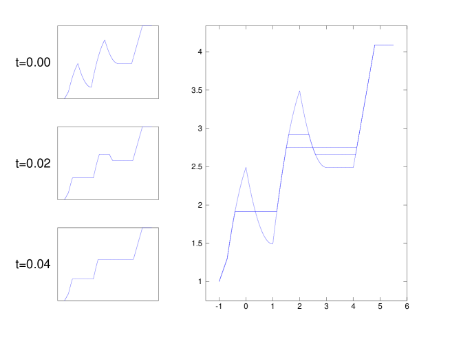
Figure 1: The first example

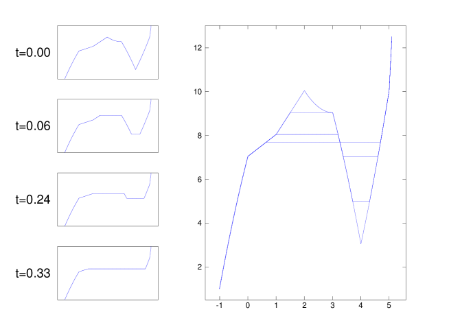
Figure 2: The second example

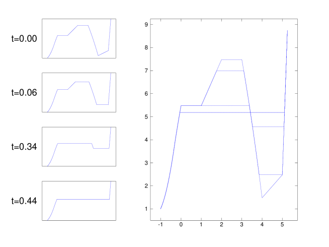
Figure 3: The third example

Observe that, all degenerated facets disappear after the first step of evolution. The number of regular facets that may appear is limited by their number and the overall number of regular facets decreases from the second step of evolution. The flat area broadens with each step. All solutions remain continuous and their $||\cdot||_{L_{\infty}}$ norm is bounded by the norm of initial data.

Acknowledgment PR thanks Professor José Mazón for inspiring conversations on the topic of this paper which lead to an improvement of the proof of Theorem 5.1. Special thanks go to the Iberia airline for creating extra opportunities to work on this paper and on related topics. The work has been partly supported by MN grant No. N N201 268935.

References

• [Al] W.K.Allard, Total Variation Regularization for Image Denoising, I. Geometric theory, SIAM J. Math. Anal. 39 (2007/08), no. 4, 1150–1190.
• [ABC] F.Andreu, C.Ballester, V.Caselles, J.M. MazΓ³n, The Dirichlet problem for the total variation flow. J. Funct. Anal. 180, (2001), 347–403
• [ABa] F.Andreu, C.Ballester, V.Caselles, J.M.MazΓ³n, J.M.: Minimizing total variation flow. Diff. Int. Equations, 14, 321–360 (2001), 321–360.
• [AG] S.Angenent, M.E.Gurtin, Multiphase thermomechanics with interfacial structure. II. Evolution of an isothermal interface. Arch. Rational Mech. Anal. 108, (1989), no. 4, 323–391.
• [ABu] H.Attouch, G.Buttazzo, G.Michaille, Variational analysis in Sobolev and BV spaces. Applications to PDEs and optimization. MPS/SIAM Series on Optimization 6. Philadelphia, PA, SIAM. Philadelphia, 2006.
• [AC1] F.Andreu-Vaillo, V.Caselles, V., J.M.MazΓ³n, Parabolic quasilinear equations minimizing linear growth functionals. BirkhΓ€user, Basel, 2004
• [AC2] F.Andreu, V.Caselles, J.M.MazΓ³n, S.Moll, The Dirichlet problem associated to the relativistic heat equation, Math. Ann., 347, (2010), 135-199.
• [Az] G.Anzellotti, Pairings between measures and bounded functions and compensated compactness. Ann. Mat. Pura Appl. (4) 135 (1983), 293–318.
• [ACD] F.Andreu, V.Caselles, J.I.DΓ­az, J.M.MazΓ³n, Some qualitative properties for the total variation flow. J. Funct. Anal. 188, (2002), 516–547
• [Ba] V.Barbu, β€œNonlinear semigroups and differential equations in Banach spaces” Leyden, The Netherlands: Noordhoff International Publishing, 1976.
• [BL] P.Belik, M.Luskin, A total-variation surface energy model for thin films of martensitic crystals. Interfaces Free Bound., 4, (2002), 71–88
• [BCN] G.Bellettini, V.Caselles, M.Novaga, The total variation flow in $\mathbb{R}^{N}$. J. Diff. Eqns. , 184, (2002), 475–525
• [Br] H.BrΓ©zis, OpΓ©rateurs maximaux monotones et semi-groupes de contractions dans les espaces de Hilbert. Amsterdam-London: North-Holland Publishing, 1973.
• [Cg] K.-Ch.Chang, Variational methods for non-differentiable functionals and their applications to Partial Differential Equations, J. Math. Anal. Appl., 80, (1981), 102–129.
• [CL] M.G.Crandall, T.M.Liggett, Generation of semi-groups of nonlinear transformations on general Banach spaces. Amer. J. Math. 93, (1971), 265–298.
• [dB] G.diBlasio, Differtiability of Spatially Homogeneous Solution of the Boltzmann Equation in the Non Maxwellian Case. Commun. Math. Phys. 38, (1974), 331–340.
• [FOP] X.Feng, M.Oehsen, A.Prohl, Rate of convergence of regularization procedures and finite element approximations for the total variation flow. Numer. Math., 100 (2005), no. 3, 441–456.
• [FG] T.Fukui, Y.Giga, Motion of a graph by nonsmooth weighted curvature. (English summary) World Congress of Nonlinear Analysts ’92, Vol. I–IV (Tampa, FL, 1992), 47–56, de Gruyter, Berlin, 1996.
• [GG] M.-H.Giga, Y.Giga, Very singular diffusion equations: second and fourth order problems Japan J. Indust. Appl. Math. , 27, (2010), 323–345.
• [GGR] M.-H.Giga, Y.Giga, P.Rybka, A comparison principle for singular diffusion equations with spatially inhomogeneous driving force, in preparation.
• [GGK] M.-H.Giga, Y.Giga, R.Kobayashi, Very Singular Diffusion Equations, Advanced Studies in Pure Mathematics 31, 2001 Taniguchi Conference on Mathematics Nara ’98 93-125
• [KG] R.Kobayashi, Y.Giga, Equations with Singular Diffusivity, Journal of Statistical Physics, 95, Nos. 5/6, (1999), 1197–1220.
• [M] P.B.Mucha, Global existence for the Einstein-Boltzmann equation in the flat Robertson-Walker spacetime. Comm. Math. Phys., 203 (1999), no. 1, 107–118.
• [MR1] P.B.Mucha, P.Rybka, A new look at equilibria in Stefan type problems in the plane, SIAM J. Math. Anal. 39, No. 4, (2007), 1120-1134.
• [MR2] P.B.Mucha, P.Rybka, A caricature of a singular curvature flow in the plane, Nonlinearity, 21, (2008), 2281-2316.
• [MR3] P.B.Mucha, P.Rybka, Almost classical solutions of static Stefan type problems involving crystalline curvature, in: "Nonlocal and Abstract Parabolic Equations and their Applications", Banach Center Publ. 86, IMPAN, Warszawa, 2009, 223-234.
• [Ma] J.Quah, D.Margetis, Anisotropic diffusion in continuum relaxation of stepped crystal surfaces, J. Phys. A: Math. Theor. 41 (2008) 235004 (18pp)
• [ROF] L.I.Rudin, S.Osher, E.Fatemi, Nonlinear total variation based noise removal argorithms, Physica D, 60, (1992), 259–268.
• [Ta] J.Taylor, Motion of curves by crystalline curvature, including triple junctions and boundary points, In: Differential Geometry: Partial Differential Equations on Manifolds (eds. R. Greene and S. T. Yau), Proc. Symp. Pure Math., 54 (1993) Part I, pp.417-438, Amer. Math. Society Providence, RI.
• [TGO] Y.H.R.Tsai, Y.Giga, S.Osher, A level set approach for computing discontinuous solutions of Hamilton-Jacobi equations. Math. Comp. . 72 (2003), no. 241, 159–181.
• [Z] W.P.Ziemer, β€œWeakly differentiable functions”, Springer, New York, 1989.