Experimental study of fragmentation products in the reactions ¹¹²Sn + ¹¹²Sn
and ¹²⁴Sn + ¹²⁴Sn at 1$\cdot A$ GeV

Abstract

Production cross-sections and longitudinal velocity distributions of the projectile-like residues produced in the reactions ¹¹²Sn + ¹¹²Sn and ¹²⁴Sn + ¹²⁴Sn both at an incident beam energy of 1$\cdot A$ GeV were measured with the high-resolution magnetic spectrometer, the Fragment Separator (FRS) of GSI. For both reactions the characteristics of the velocity distributions and nuclide production cross sections were determined for residues with atomic number $Z$ $\geq$ 10. A comparison of the results of the two reactions is presented.

I introduction

Since heavy-ion beams at relativistic energies $E$ $>$100$\cdot A$ MeV became available in laboratories PhysRevLett.52.180 ; Kienle1988277 , a possibility to study static and dynamic properties of nuclear matter over a wide range of temperature and density has been opened annurev.ns.28.120178 ; Pochodzalla:1997vq . Depending on the impact parameter $b$, heavy-ion collisions can be divided into three groups PhysRev.75.1779 :

One extreme are central collisions in which projectile and target completely overlap. In this type of collisions, high densities and high excitation energies can be achieved Bertsch1988189 , and thus they appear to be an excellent tool to study the equation of state of hot and compressed nuclear matter as well as in-medium nucleon-nucleon interactions. To this goal, immense experimental effort has been, and is still being, invested to measure for example the flow pattern of nucleons and particles, kaon production or charged-particles correlation in central heavy-ion collisions Reisdorf:1997fx ; Senger:2004xa ; Reisdorf2010366 . Since high densities and high excitation energies are achieved only for short time intervals of the order $10^{-22}$ s and in volumes of the order 100 fm³ Cubero1990345 , it is mandatory to understand the complete dynamic evolution of the reaction in order to extract the information on the nuclear equation of state under these extreme conditions. This is still not an easy task.

An other extreme is the case of large impact parameters leading to very peripheral collisions. This type of collisions is characterized by a small mass loss in projectile and/or target and rather low excitation energies. Projectile-like fragments move with velocities very close to the original one of the projectile. These collisions have been proved to be an excellent tool to study e.g. nuclear-structure effects at large deformations Schmidt2000221 ; Steinhauser199889 ; Rejmund2000215 or neutron skin PhysRevC.76.051603 .

For the intermediate range of impact parameters, a considerable amount of excitation energy Schmidt1993313 and a slight linear momentum transfer are induced, but compression is small. Thus, the mid-peripheral heavy-ion collisions at relativistic energies are an ideal scenario for studying multifragment decay of the spectator matter due to purely thermal instabilities Schuttauf1996457 , avoiding any compression effect. Multifragmentation reactions have been extensively studied in order to search for the signals of the liquid-gas phase transition in finite nuclear systems Pochodzalla:1997vq ; PhysRevLett.75.1040 ; Trautmann2005407 . Since some time, isotopic effects in multifragmentation reactions also gained a lot of interest PhysRevC.65.044610 ; PhysRevLett.102.122701 ; PhysRevLett.102.142503 ; trautmann2008 , as neutron-star models or supernova simulations demand a nuclear equation of state similar to those met in mid-peripheral relativistic heavy-ion collisions PhysRevLett.72.2835 ; Dean1995429 ; Botvina2004233 . Similar to the experiments where central collisions are studied, a lot of effort is invested in developing devices covering the full solid angle in order to attain particle multiplicities as well as correlations between observed particles.

Recently, high-resolution experiments on kinematical properties of projectile residues produced in mid-peripheral heavy-ion collisions have been proposed as a new tool to study the nonlocal properties of the nuclear force PhysRevC.64.034601 ; PhysRevLett.90.212302 . According to the model calculations PhysRevC.64.034601 , the transversal and the longitudinal momentum distributions of the spectator matter surviving the collisional stage are influenced by the participant blast, occurring after the compression phase in the colliding zone. Consequently, the momentum distributions of spectator residues in mid-peripheral collisions should be sensitive to the nuclear force. In order to yield conclusive results, the momentum distributions of projectile residues have to be measured with high precision. This can only be achieved with high-resolution magnetic spectrometers, as experimental set-ups covering full solid angle do not have the required resolution.

Unfortunately, detailed experimental information on kinematical properties of projectile residues produced in heavy-ion collisions at relativistic energies is rather lacking. In a review on measured mean velocities of spectator-like fragments presented by Morrissey in 1989 PhysRevC.39.460 a clear correlation between the observed momentum shift with the mass loss in very peripheral collisions has been observed. This shift has been interpreted as the consequence of friction in the nucleus-nucleus collision PhysRevC.39.460 ; AbulMagd1976327 . On the other hand, the momentum distributions of lighter fragments, with a mass loss larger than about one-third of the mass of the projectile, respectively, the target nucleus, showed a large spreading with no clear tendency. Since then, a lot of new data on the momentum distributions have been measured, but unfortunately only few of them cover the whole range - from projectile down to the lowest nuclear charges of produced fragments Weber1994659 ; PhysRevC.70.054607 ; PhysRevC.76.064609 ; PhysRevC.78.044616 . To overcome this lack of high-precision data on the velocities of projectile fragments, a dedicated experimental campaign PhysRevLett.90.212302 ; vladimir has been started at GSI using the heavy-ion accelerator SIS18 and the Fragment Separator (FRS).

The present work represents the next step in this campaign, and is dedicated to a study of the influence of the isotopic composition of the projectile on the kinematical properties of projectile residues in peripheral and mid-peripheral relativistic heavy-ion collisions. To this goal, two symmetric systems ¹¹²Sn+¹¹²Sn and ¹²⁴Sn+¹²⁴Sn at the projectile energy of 1$\cdot A$ GeV have been studied. The $N$/$Z$ ratio of ¹¹²Sn is 1.24, and the one of ¹²⁴Sn is 1.48, resulting, for a given $Z$, in the largest span in $N$/$Z$ values for stable nuclei in this mass range. For this exploratory study the beams of stable nuclei have been chosen as their emittance is smaller than in case of secondary beams, while available intensities are higher. Since in both reactions the target and projectile are the same nuclei, the $N$/$Z$ stays homogeneous for all possible impact parameters, despite the small effects coming from the neutron skin. This $N$/$Z$ value is determined entirely by the corresponding tin nuclei in the system. The incident energy is chosen in such way to have the best conditions for the transmission of the reaction products through the FRS.

In addition to the high-precision data on the longitudinal velocity of the projectile fragments, also the production cross sections have been measured.

The present work is ordered in the following way: In section II we describe the experimental approach and the data analysis. In section III velocity distribution of the final residues, as well as the moments of this distribution are presented. In section IV production cross sections of the projectile residues measured in these two reactions are given. Detailed discussion on the physics behind the data as well as comparison with different theoretical predictions is a topic of forthcoming publications, and will not be discussed here.

II Experiment and data analysis

In this section details on the experimental set-up as well as steps needed to be undertaken to obtain the velocity distributions and production cross sections of all the projectile-like residues will be presented.

II.1 Experimental technique

The experiment was performed at GSI, Darmstadt, with two systems: ¹¹²Sn + ¹¹²Sn and ¹²⁴Sn + ¹²⁴Sn both at an incident beam energy of 1$\cdot A$ GeV. Beams were delivered from the universal linear accelerator (UNILAC) to the SIS18 heavy-ion synchrotron where they were extracted and guided through the target area to the FRagment Separator (FRS) Geissel:1991zn . The FRS is a two-stage magnetic spectrometer with a maximum bending power of 18 Tm, an angular acceptance of 15 mrad around the beam axis, and a momentum acceptance of 3%. The FRS was used for the separation and analysis of the reaction products. In Fig. 1 a schematic view of the experimental setup is shown with all the detectors used in the experiment. The two tin beams impinged on the tin targets whose isotopic composition closely corresponded to the nuclei of the beam: a 126.7 $\pm$ 0.6 mg/cm² thick ¹¹²Sn target with 99.5$\pm$0.2 enrichment and a 141.8 $\pm$ 0.7 mg/cm² thick ¹²⁴Sn target with 97.5$\pm$0.2 enrichment. Due to the high linear momenta of the incoming projectiles, most of the produced projectile-like fragments escaped the target in forward direction and were then analyzed by the fragment separator FRS, used as a momentum-loss achromat.

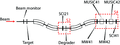
Figure 1: (Color online) Schematic view of the Fragment Separator (FRS) and the associated detector equipments. The notation of different detectors is explained in the text.

The scintillation detectors were used to acquire the horizontal position of the passing ions and to register the start and the stop time signals for the time-of-flight (ToF) measurement. The uncertainty in the position determination was about 3 mm (FWHM), and in ToF it amounted to 100 ps (FWHM). One scintillation detector was placed at the end of the first stage at the intermediate focal plane S2 and another one at the end of the second stage at the final focal plane S4.

The radius of the fragment trajectory $\rho$ is measured with a relative uncertainty of about $4\cdot 10^{-4}$. The magnetic field strength $B$ is measured with high precision ($\Delta B/B\sim 10^{-4}$) using the Hall probes. In this way, one can obtain a measure of the magnetic rigidity $B\rho$ with a resolution of about 5$\cdot$10^-4. Together with the longitudinal velocity, determined from the ToF measurement, the mass-over-charge ratio $A$/$Z$ of the fragments could be determined according to the formula:

$$\frac{A}{Z}=\frac{1}{c}\cdot\frac{e}{m_{0}+\delta m}\cdot\frac{B\rho}{\beta\gamma},$$ (1)

where $c$ is the velocity of light, $e$ the elementary charge, $m_{0}$ atomic mass unit, $\delta m=dM/A$ the mass excess per nucleon, $\gamma=\sqrt{(1-\beta^{2})^{-1}}$ the Lorentz factor, $\beta=v/c$ velocity in natural units, where $v$ is the longitudinal velocity of the fragment obtained from the ToF measurement. For the calculation of the mass excess a generalized empirical mass formula was used Myers19661 , which provided sufficient accuracy for the $A/Z$ calculation.

Due to their high velocity, the fragments were completely stripped of electrons with a probability higher than 99% Stohlker1991408 , so that the charge of the passing ion $Q$ coincides with the atomic number of the fragment $Z$. At the end of the second stage the ions were detected by two multiple-sampling ionization chambers (MUSICs) Pfutzner1994213 . The MUSICs provided the energy-loss signals which were used to obtain the information on nuclear charge $Z$. Drift-time signals from the two MUSIC detectors also provided information on the horizontal position and the horizontal angle of the passing ions trajectory. This information was used to determine the length of the ions path between the scintillators which then allowed the determination of the velocity together with the ToF information. The nuclear-charge resolution has been improved by correcting the energy-loss signal for the position and velocity dependence as discussed in e.g. ref. PhysRevC.78.044616 . In Fig. 2, the Z spectrum deduced from the MUSIC energy-loss is shown before and after these corrections. The improvement in the resolution is especially seen for the higher nuclear charges. The atomic number $Z$ was determined with an uncertainty of $\Delta Z=0.4$ units (FWHM). In order to prevent the overloading of the MUSIC detectors with fragments produced with high counting rates i.e. light particles, the threshold on the signals collected from the MUSICs was set so that the fragments with nuclear charge $Z\geq$ 10 were fully recorded.

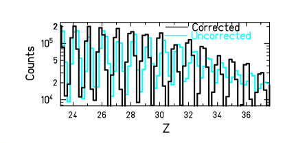
Figure 2: (Color online) MUSIC charge resolution before (light blue) and after various corrections described in the text (black).

Due to the limited momentum acceptance of $\Delta p/p\cong\pm$ 1.5% of the fragment separator several magnetic settings were required to scan the full momentum distributions of the projectile residues. The term ”magnetic setting” refers to a measurement performed with given magnetic-field values in the magnets. The setting thus determines the acceptance of particles, with certain range of magnetic rigidities, that are able to pass the FRS.

In some settings an additional degrader is added in between the two stages of the FRS. This is beneficial when measuring fragments produced with low yields. In these settings one can increase the intensity of the beam without overloading the detectors with fragments produced with higher counting rates and thus obtain a proper statistics for all the fragments. In both systems the settings that were devoted to measure the lighter residues, $Z$ $\leq$ 35, where measured with the aluminum degrader with a thickness of (737.1 $\pm$ 1) mg$\cdot$ cm^-2.

The recognition pattern, formed by plotting the $A$/$Z$ ratio versus the charge of the fragments produced in both experiments is presented in Fig. 3. Settings dedicated for the measurement of light residues are given separately from the heavy-residue recognition plots. The gaps in the recognition pattern appear due to the necessity to protect the detectors against the primary beam. Therefore, a number of nuclei with magnetic rigidities very close to the beam were not measured. Each spot in Fig. 3 represents one nucleus with a given $A$ and $Z$. Using the characteristic pattern for $N=Z$ nuclei, i.e. vertical line at $A/Z=2$ and also the measurements with the primary beam, the full identification of all the residues has been performed. The achieved resolution in mass was $\Delta A/A=4\cdot 10^{-3}$.

$\begin{array}[]{c}\mbox{\bf${}^{112}$Sn + ${}^{112}$Sn}\\ \includegraphics[width=216.81pt]{Q-VS_AQTIGHT_112SN.EPS}\\ \mbox{\bf${}^{124}$Sn + ${}^{124}$Sn}\\ \includegraphics[width=216.81pt]{Q-VS_AQTIGHT_124SN.EPS}\\ \end{array}$

Figure 3: (Color online) Recognition patterns of fragments formed in ¹¹²Sn + ¹¹²Sn (top) and in ¹²⁴Sn + ¹²⁴Sn (bottom) reactions. Settings measured with degrader (left) are shown separately from those obtained without degrader (right). Color code represents yields on the logarithmic scale.

Once the fragments were isotopically identified in nuclear mass $A$ and nuclear charge $Z$, equation 1 could be used to extract the longitudinal velocity from the known $B\rho$ values at S2. In this way, the resolution in the longitudinal velocity is given only by the resolution in the magnetic rigidity, as $A$ and $Z$ are integer numbers and thus contain no uncertainty, and amounts to $\Delta v/v=10^{-4}$ representing about one order of magnitude improvement relative to the resolution obtained via ToF measurement. Thus, in the following, we will use the velocity distributions obtained via ”$B\rho$ measurement”.

II.2 Data analysis

II.2.1 Reconstruction of full velocity distributions

As mentioned earlier, the FRS momentum acceptance in each setting is $\pm$ 1.5% of the magnetic rigidity ($B\rho$) of the selected central trajectory. For each setting, the magnetic fields of the dipoles were scaled by steps of 1.5% to assure a sufficient overlap of the velocity distributions measured in the neighboring settings. Especially for lighter nuclei ($Z$ $<$ 30), the velocity distributions are generally always wider then what one can measure in one setting, and it is necessary to combine data from several measurements with different magnetic rigidities to cover the full range of velocities of each fragment.

Data obtained from different settings have to be normalized to the primary-beam intensity, and corrected for the limited angular acceptance and dead-time of the data-acquisition system before being merged. These different corrections are described below.

The normalization to the primary-beam intensity was done by counting the number of the incoming beam particles using the signal from the beam-current transformer (TRAFO) Reeg2001 used for the SIS beam monitoring. The advantage of using the TRAFO instead of the standard FRS beam monitor, SEETRAM (Secondary Electron TRAnsmission Monitor) Junghans1996312 ; Jurado2002603 , is the fact that there is no layer of matter introduced to the beam line, which would act as an additional target. However the SEETRAM output served as an intermediate information to connect the absolute calibration with the scintillator to the TRAFO output. SEETRAM measures the electron current as a function of the number of incident beam particles which is measured with a scintillation detector during the calibration run. Due to the saturation of the scintillation detector output at large particle fluxes the calibration was made up to the particle rate in the order of $\sim$10⁵ particles per second. The calibration data and a quadratic fit are presented in Fig. 4. Since SEETRAM itself does not suffer any sizable saturation at these particle rates, the linear term of the quadratic fits where taken as the calibration factor to compensate the scintillator saturation. TRAFO could not measure the low intensity particle flux used in the SEETRAM calibration, so TRAFO was calibrated with higher beam intensity against the calibrated SEETRAM output. The linear calibration fit of TRAFO is presented in Fig. 4.

$\begin{array}[]{c}\includegraphics[width=195.12767pt]{SCI01.EPS}\\ \includegraphics[width=195.12767pt]{trafo.EPS}\\ \end{array}$

Figure 4: Top: Dashed line shows the quadratic calibration curve fitted to the data showing scintillator counts versus the SEETRAM output. Solid line shows the linear part of the fit. Bottom: Linear calibration fit to the data showing the SEETRAM output versus the TRAFO output.

The next step undertaken before merging the velocities measured in different magnetic-field settings was the correction for the slight variation of the angular transmission as a function of the ion’s magnetic rigidities in the first and second halves of the FRS Benlliure2002493 . While the heavy residues are produced with rather narrow angular distributions and they are fully transmitted through the FRS, the angular distributions of light residues are rather broad, and the angular transmission of these residues may be as low as 10%. The angular transmission of the FRS has been under intense investigation in many experiments in the past. For the case of fragmentation reactions, a detailed description of the transmission of each ion species through the magnetic fields of FRS is given in ref. Benlliure2002493 . In the same work, also an algorithm for correcting for the transmission losses due to the limited angular acceptance is given. This algorithm has been adapted in the present work. After this correction the velocity distributions closely represent the distributions inside the afore mentioned angular acceptance of the spectrometer (15 mrad around the beam axis). The applied transmission correction factors were assumed to have a relative uncertainty of 15%. In the present experiment, the dead-time of the data-acquisition system was varying, depending on the counting rate, between 2% and 50%. For each setting, the dead-time values have been registered, and measured counting rates consequently corrected for.

Fig. 5 illustrates the reconstruction of the velocity distribution of ²²Ne obtained from merging single settings after performing above-mentioned corrections.

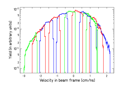
Figure 5: (Color online) Reconstructed velocity distribution of the nuclide $A$=21, $Z$=10 of the ¹²⁴Sn + ¹²⁴Sn system inside an acceptance angle of 15 mrad. Contributions of measurements with different magnetic-field settings are shown.

II.2.2 Determination of the production cross sections

At this place we will describe how the production cross section of each nuclide was obtained from its reconstructed velocity distribution.

For the evaluations of the production cross sections, the part of the velocity distributions outside the angular acceptance needed to be estimated. The estimation was based on the isotropy assumption from which it follows that the overall velocity distributions in three-dimensional space have the same standard deviation as the reconstructed longitudinal velocity distributions inside the angular acceptance of the spectrometer. This procedure is especially reliable for the narrow distributions of the heavy residues but the cross sections of the light residues (Z $\lesssim$ 14) may have been somewhat underestimated due to the shape asymmetries in their velocity distributions.

The integral of the reconstructed velocity distribution of a given fragment was used as a basis to obtain its production cross section. This is done in the following way: The yield $Y(A,Z)$ of a given residue is obtained by integrating its completely reconstructed velocity distribution. By this method one ensures that there is no double counting due to the overlap of the neighboring magnetic-field settings.

The determination of production cross sections $\sigma(A,Z)$ from the measured yield $Y(A,Z)$ of single nuclide $(A,Z)$ is calculated as:

$$\sigma(A,Z)=\frac{Y(A,Z)\cdot\alpha}{N_{Sn}},$$ (2)

where $\alpha$ is a correction factor for the losses due to secondary reactions in scintillator and degrader, and $N_{Sn}$ is the number of target nuclei over unit area.

The function $\alpha$, plotted in Fig. 6, is a quadratic fit made to the correction factors calculated with the code AMADEUS AMA for every ten atomic mass units. AMADEUS gives the percentage of nuclear reactions in matter for a given fragment with a given velocity. Corrections ranging from 0.5% to 8% were applied. We assume a relative uncertainty of 10% for the correction for secondary reactions. Please note, that no corrections due to the secondary reactions in the targets were needed, as both targets were very thin, and the probability for a fragment to react in one of the targets was less than 0.1%.

The number of target nuclei over unit area $N_{Sn}$ is equal to the number of individual scattering centers per unit volume, $n$, times the thickness, $x$, of the target:

$$N_{Sn}=n\cdot x=\frac{\rho\cdot N_{Av}}{M}\cdot\frac{T}{\rho}=\frac{N_{Av}\cdot T}{M}\textrm{,}$$ (3)

where $T$ is the density thickness of the target in mg $\cdot$ cm^-2, $N_{Av}$ = 6.022$\cdot$10²³mol^-1 Avogadro’s number, $M$ the atomic weight of the target material [mg$\cdot$ mol^-1] and $\rho$ the density [mg$\cdot$ cm^-3] of the target material. Numerical values for the quantities in the equation 3 are given in table 1 for both tin targets used in the experiment.

target	$T$ [mg$\cdot$ cm-2]	$M$ [g$\cdot$ mol-1]	Enrichment [%]
112Sn	126.7 $\pm$ 0.6	112.4 $\pm$ 0.2	99.5$\pm$0.2
124Sn	141.8 $\pm$ 0.7	123.9 $\pm$ 0.2	97.5$\pm$0.2

Table 1: Numerical values used in the equation 3.

Figure 6: Secondary-reaction correction factor in different layers of matter obtained from AMADEUS AMA calculation.

Finally, to ensure that each count in the distribution corresponding to given $A$ and $Z$ in the identification plot indeed represents this isotope and does not come from products of ionic charge-changing processes and secondary reactions in the detector materials and degrader in the beam line, all spectra were accumulated under the condition that each measured fragment had the same ratio $A$/$Q$ in both stages of the FRS. Due to this constraint on the $A$/$Q$ ratio the ions which undergo ionic charge-changing processes and which are responsible for the most of the contaminants can be suppressed efficiently. The amount of remaining contaminants from background of secondary-reaction products which were transmitted to the final image plane and fulfilled the constraint on the $A$/$Q$ and on the energy loss in the ionization chamber, was estimated to be less then 1%. More details can be found in ref. Enqvist2002435 .

III Results and discussion

With the method described in the previous chapter we obtained the longitudinal velocity distributions of the projectile residues fully identified in mass and atomic number in the reactions ¹¹²Sn + ¹¹²Sn and ¹²⁴Sn + ¹²⁴Sn at an incident beam energy 1$\cdot A$ GeV. The width and the mean value of the velocity distributions as well as the production cross sections were determined, and will be presented.

III.1 Velocity distributions and their moments

In Fig. 7 and in Fig. 8 some examples of the measured distributions of longitudinal velocity inside an angular acceptance range of 15 mrad around the beam direction in the frame of the projectile are presented for few selected nuclides.

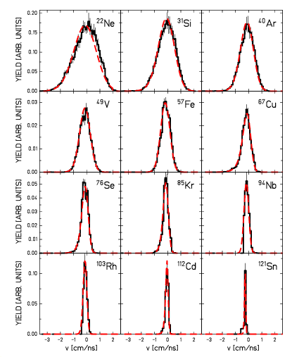
Figure 7: (Color online) Velocity distributions in the rest frame of the projectile for several nuclides measured in the reaction ¹²⁴Sn + ¹²⁴Sn. The fitted functions are shown as dashed red lines. Distributions represent velocities inside an angular range of 15 mrad.

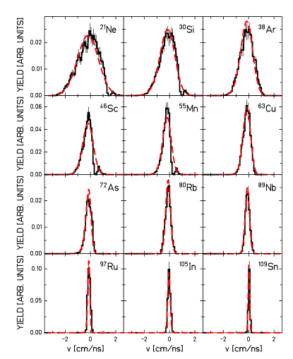
Figure 8: (Color online) Velocity distributions in the rest frame of the projectile for several nuclides measured in the reaction ¹¹²Sn + ¹¹²Sn. The fitted functions are shown as dashed red lines. Distributions represent velocities inside an angular range of 15 mrad.

By observing the general shapes of the velocity distributions and without going into details of different reaction mechanisms, one can explain the general features in terms of abrasion-ablation model Gaimard1991709 . In this model the heavy fragments shown in Fig. 7 and in Fig. 8 are produced in peripheral collisions with small overlap between the projectile and the target nucleus. This results in a formation of slightly excited prefragments, which then de-excite via evaporation of neutrons, light charged particles and light clusters. As the number of abraded nucleons is small, the fluctuations in the velocity distribution of created prefragments are also small Goldhaber1974306 , and consequent evaporation stage only slightly increases the width of the velocity distribution. Thus, these residues show narrow velocity distributions with the mean value only slightly lower than that of the beam particles. Lighter residues are presumably produced at smaller impact parameters, where the introduced excitation energy can be high enough for thermal instabilities to set in Botvina1995737 ; Schuttauf1996457 . These residues portray wider velocity distributions, indicating a larger number of abraded and evaporated nucleons. For all the residues, the longitudinal velocity distributions show Gaussian-like shape with a slightly enhanced tail in the slower side in case of the lighter residues. This asymmetry in the shape of velocity distributions of the lightest residues shows, as discussed in references Ricciardi:2005ht ; PhysRevC.70.054607 ; PhysRevC.78.044616 that these fragments have been produced via different reaction mechanisms like e.g. simultaneous and/or sequential decay.

For the sake of more quantitative analysis, the distributions were fitted with one Gaussian with an exponential tail. This fitting function was chosen because it resembled the experimental data sufficiently well. Advantage of the fitting was to get rid of some unwanted features of the distributions that were introduced only due to experimental limitations. Some of the velocity distributions show, especially in the case of ¹¹²Sn + ¹¹²Sn, cuts caused by slits, which were inserted to protect the detectors from the primary beam and its first two charge states; see e.g. ²¹Ne, ³⁰Si, ⁴⁶Sc or ⁵⁵Mn in Fig. 8. The fitting procedure could, thus, recover some of the incompletely measured velocity distributions. The uncertainty introduced by this fitting procedure is typically of the order of 2% for each extracted parameter.

In Fig. 9 the width, standard deviation $\sigma_{\|}$ of the fitted Gaussian function with exponential tail, is given for the longitudinal momentum distributions for all fragments measured in two reactions. Also shown are a theoretical prediction Bacquias and the empirical parametrization of Morrissey PhysRevC.39.460 .

$\begin{array}[]{c}\includegraphics[width=195.12767pt]{112SN_SIGMAVSPREDICTION.EPS}\\ \includegraphics[width=195.12767pt]{124SN_SIGMAVSPREDICTION.EPS}\\ \end{array}$

Figure 9: Standard deviation of the Gaussian part of the fitted functions to the fragment momentum distributions for both systems; ¹¹²Sn(1$\cdot A$ GeV)+¹¹²Sn (upper diagram) and ¹²⁴Sn(1$\cdot A$ GeV)+¹²⁴Sn (lower diagram). The values are given in momentum units [MeV/c]. Given curves present the prediction of theoretical model Bacquias and the empirical parametrization by Morrissey PhysRevC.39.460 .

From these figures we see that the width of the measured longitudinal momentum distributions first increase with decreasing mass of the final residue. The maximum is reached for the final-fragment mass close to half the mass of the projectile. For lower masses, the width then decreases. Uncertainties for the standard deviations are given by the fitting routine which calculates them according to the uncertainties of each bin content of the velocity distributions. The total uncertainty for each bin content were calculated from individual error sources by using the error propagation law. This uncertainty consist of both statistical and systematic. Other uncertainties that might have not been considered have no sizable contribution, when added quadratically to the estimated ones, since they are in total less than 3%.

According to the statistical model of Goldhaber Goldhaber1974306 , the longitudinal momentum of the projectile-like fragments after the first reaction stage are determined by the intrinsic Fermi motion of the constituent nucleons which are removed from the projectile during the abrasion process. In this model the individual nucleons within the projectile have their own momenta that sum up to zero in the rest frame of the projectile. The abrasion stage then removes nucleons with no preference with respect to their momentum, and the sum of the momenta of the remaining nucleons in the prefragment may not sum up to zero anymore. Due to the momentum conservation, the sum of momenta of abraded nucleons, has to be opposite to the momentum of the prefragment. More nucleons are removed in abrasion more fluctuations of the remaining total momentum may occur, and the maximum is reached for masses equal the half of the mass of the projectile. By this model, the projectile remnants end up with three-dimensional Gaussian-shape momentum distributions, whose widths are determined by the number of removed nucleons. Although it considers only the abrasion stage, the Goldhaber’s model Goldhaber1974306 has often been used in interpreting experimental results. Recently, Goldhaber’s model has been refined and the influence of different decay stages, i.e. simultaneous and/or sequential decay, has been incorporated in the description of the momentum dispersion of final fragmentation residues Bacquias . This has resulted in an improved description of the width of the momentum distribution of fragmentation residues.

The projectile remnant subsequently enters, depending on the excitation energy induced in the abrasion stage, the stage of simultaneous and/or sequential decay. These decay stages introduce additional fluctuations in the momentum distribution as discussed in ref. Bacquias .

Another often used description of the momentum width is based on the empirical approach of Morrissey PhysRevC.39.460 . Although this approach describes very well the width of the momentum distribution close to the projectile, it fails severely for the masses smaller than the half of the projectile mass, see Fig. 9.

Another characteristic of the velocity distribution is its mean value. In Fig. 10 we present the average mean velocity in the frame of the projectile for each mass number of the fragmentation residues ($A_{frag}$) produced in the reactions induced by ¹²⁴Sn and ¹¹²Sn, as a function of their relative mass loss defined as $(A_{frag}-A_{proj})/A_{proj}$. Uncertainties of the mean values are also based on the uncertainties of each bin of the velocity distributions and were given by the fitting routine. In addition to this, the uncertainty of the mean value contains the uncertainty in determining the velocity of the primary beam since the mean values are given in the beam frame.

In Fig. 10 the dashed line shows the expected mean velocities according to the systematics of Morrissey PhysRevC.39.460 .

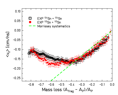
Figure 10: (Color online) Mean value of the longitudinal velocity distributions in the frame of the projectile of residues produced in the reactions ¹²⁴Sn (1$\cdot A$ GeV)+ ¹²⁴Sn (open squares) and ¹¹²Sn (1$\cdot A$ GeV) + ¹¹²Sn (filled circles) as a function of their relative mass loss. The mean values represent the mean velocities inside an angular range of 15 mrad.

The mean value represents the overall velocity shift induced in these reactions. A similar pattern is observed in both systems. Residues close to the projectile show a clear decrease of the mean velocity with their mass loss which closely follows the systematics of Morrissey PhysRevC.39.460 . For this region, there is also no difference between the mean velocities in the two systems. The Morrissey systematics does not contain any interpretation about the reaction mechanism, it is just a fit made to the available data at that time. Nevertheless, this behavior can be explained by simple two-body interaction, namely friction, between the projectile and target nuclei in peripheral heavy-ion collisions. Friction appears as a consequence of interactions between the projectile and target matter in the overlapping region, and leads to a conversion of relative kinetic energy into excitation energy of projectile and target spectators. Due to this loss in kinetic energy, the velocity of spectator residues is slightly shifted towards the velocity of the reaction partner, i.e. projectile residues are slowed down AbulMagd1976327 ; Weber1994659 .

However, in less peripheral collisions, the two-body kinematics is no longer applicable since there occurs a formation of participant zone and the projectile and target spectators emit particles. In Fig. 10 at relative mass losses around 0.4, corresponding to $A\approx$ 67 and $A\approx$ 74 in ¹¹²Sn + ¹¹²Sn and in ¹²⁴Sn + ¹²⁴Sn, respectively, the mean velocity levels off and for large mass losses the mean velocity starts to rise again. This is in clear contrast with the friction picture, according to which one would expect more kinetic-energy dissipation as the mass of the residue is decreasing and, thus, lower velocity. As discussed in refs. PhysRevC.64.034601 ; PhysRevLett.90.212302 this leveling-off and increase in the mean velocity of the final residue with decreasing mass can be the evidence of the influence of the participant blast on the properties of the projectile-like spectator. For the lowest masses with more than 0.5 relative mass loss the data suggest that there is also a small deviation between the two systems.

At this place, we would like to make a comment concerning the influence of limited angular acceptance of the FRS. As we have said above, the angular transmission varies as a function of the ion’s magnetic rigidities in the first and second halves of the FRS. After correcting for this effect, the velocity distributions (see Figs. 7 and 8) as well as mean values (see Fig. 10) represent fragment velocity inside an angular range of 15 mrad. This is very important to keep in mind, when comparing our results with experiments performed with full-acceptance set-up. In our case, only those fragments which are emitted with rather small angles, i.e. 15 mrad around the beam axis, are measured and thus the measured velocity distributions presented here are only slightly influenced by e.g. binary-type events in which due to a strong Coulomb repulsion the produced fragments are emitted with larger angles PhysRevC.70.054607 ; PhysRevC.76.051603 ; Ricciardi:2005ht . On the contrary, in the full acceptance experiments, all products, regardless of their production mechanism, are detected and this of course lead to somewhat different shape of the velocity distribution as well as to lower average velocities. Due to this fact, effects seen in e.g. Fig. 10 are not easy to be observed in full-acceptance experiments. Discussion of this effect and comparison with theoretical predictions is a topic of a forthcoming publication and beyond the scope of the present paper.

III.2 Production cross sections

As already discussed, the velocity distributions served also to determine the production cross sections of the measured fragments. An overview of the measured production cross sections presented on the chart of nuclides is shown in Fig. 11. For several isotopes the cross sections could not be determined due to lack of statistics or because of severe cuts in the velocity distributions, or simply because of the limited range of the magnetic rigidity that was measured. Measured isotopic distributions are also plotted in Fig. 12 and numerical values of the production cross sections are given in the Appendix. Uncertainties of the cross sections are based on the uncertainty of the integral of the velocity distributions given by the fitting routine. An additional uncertainty was introduced by the estimation of the parts of the velocity distributions outside the angular acceptance. Fig. 12 also shows the cross sections obtained from the EPAX parametrization PhysRevC.61.034607 . EPAX is a semi-empirical parametrization of the cross sections of heavy residues from fragmentation reactions based on the idea that fragmentation products result from long, sequential evaporation chains, at the end of which the evaporation attractor line is reached. Fragment cross sections obtained in both experiments agree with the EPAX parametrization reasonably well.

$\begin{array}[]{c}\includegraphics[width=195.12767pt]{112CHART.EPS}\\ \includegraphics[width=195.12767pt]{124CHART.EPS}\\ \end{array}$

Figure 11: (Color online) Cross sections for both systems; ¹¹²Sn(1$\cdot A$ GeV)+¹¹²Sn (upper diagram) and ¹²⁴Sn(1$\cdot A$ GeV)+¹²⁴Sn (lower diagram).

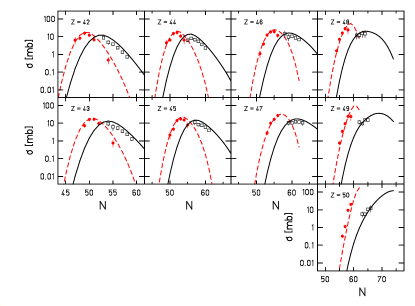
Figure 12: (Color online) Isotopic cross sections of the measured fragments in reaction ¹¹²Sn + ¹¹²Sn at 1$\cdot A$ GeV (filled dots) and in ¹²⁴Sn + ¹²⁴Sn at 1$\cdot A$ GeV (open squares). Dashed lines represents the prediction of EPAX PhysRevC.61.034607 for ¹¹²Sn + ¹¹²Sn and solid lines for ¹²⁴Sn + ¹²⁴Sn.

IV Conclusions

The high-resolving-power magnetic spectrometer, FRS, was used to measure the longitudinal velocity of the residues produced in the reactions ¹²⁴Sn + ¹²⁴Sn and ¹¹²Sn + ¹¹²Sn at 1$\cdot A$ GeV with a relative uncertainty of $\sim 1\times 10^{-4}$. This precision allows to investigate the mechanisms responsible for fragment formations. The mean value of the longitudinal velocity distributions of light projectile-like residues show a clear deviation from what one would expect on the basis of the friction picture in heavy-ion collisions.

The width of the longitudinal velocity distributions shows to deviate from the earlier empirical prediction by Morrissey PhysRevC.39.460 and is better reproduced for broader range of data by the modified Goldhaber model Bacquias which includes additional corrections to the momentum distributions due to different stages of decay.

The production cross sections were determined from the reconstructed velocity distributions. The cross sections range over several orders of magnitude from $\sim$100 $\mu$b to $\sim$30 mb with a relative uncertainty corresponding to around 20% in most cases.

Appendix A Measured data in reaction ¹²⁴Sn + ¹²⁴Sn and ¹¹²Sn + ¹¹²Sn at 1$\cdot A$ GeV.

Table 2: Production cross section of nuclides produced in reactions ¹¹²Sn + ¹¹²Sn at 1$\cdot A$ GeV. Data refers to the full production, corrected for the limited angular acceptance of the FRS.

$Z$	$A$	$\sigma$ [mb]	$Z$	$A$	$\sigma$ [mb]	$Z$	$A$	$\sigma$ [mb]	$Z$	$A$	$\sigma$ [mb]
10	21	18 $\pm$ 4	22	49	1.8 $\pm$ 0.4	31	66	5 $\pm$ 1	39	89	0.5 $\pm$ 0.2
10	22	11 $\pm$ 2	22	50	0.44 $\pm$ 0.09	31	67	8 $\pm$ 2	40	84	0.9 $\pm$ 0.2
10	23	1.9 $\pm$ 0.8	23	47	1.3 $\pm$ 0.3	31	68	6 $\pm$ 1	40	85	4 $\pm$ 1
10	24	0.9 $\pm$ 0.4	23	48	4.7 $\pm$ 0.9	31	69	2.1 $\pm$ 0.4	40	86	10 $\pm$ 2
11	23	16 $\pm$ 3	23	49	8 $\pm$ 2	31	70	1.7 $\pm$ 0.7	40	87	14 $\pm$ 3
11	24	8 $\pm$ 2	23	50	5 $\pm$ 1	31	71	0.27 $\pm$ 0.05	40	88	10 $\pm$ 2
11	25	2.9 $\pm$ 0.6	23	51	2.2 $\pm$ 0.4	32	66	0.32 $\pm$ 0.06	40	89	3.8 $\pm$ 0.8
11	26	0.8 $\pm$ 0.2	23	52	0.8 $\pm$ 0.2	32	67	1.5 $\pm$ 0.3	41	87	6 $\pm$ 2
12	25	13 $\pm$ 3	23	53	0.19 $\pm$ 0.04	32	68	4.9 $\pm$ 1.0	41	88	9 $\pm$ 2
12	26	11 $\pm$ 2	24	49	1.2 $\pm$ 0.2	32	69	8 $\pm$ 2	41	89	15 $\pm$ 3
12	27	3.8 $\pm$ 0.8	24	50	4.5 $\pm$ 0.9	32	70	7 $\pm$ 1	41	90	11 $\pm$ 2
12	28	1.0 $\pm$ 0.2	24	51	8 $\pm$ 2	32	71	2.1 $\pm$ 0.8	41	91	5 $\pm$ 1
13	27	15 $\pm$ 3	24	52	7 $\pm$ 1	32	72	1.2 $\pm$ 0.4	41	94	0.15 $\pm$ 0.04
13	28	8 $\pm$ 2	24	53	1.9 $\pm$ 0.4	32	73	0.3 $\pm$ 0.1	42	89	6 $\pm$ 3
13	29	4.4 $\pm$ 0.9	24	54	1.0 $\pm$ 0.2	33	68	0.24 $\pm$ 0.05	42	90	8 $\pm$ 2
13	30	0.6 $\pm$ 0.2	24	55	0.22 $\pm$ 0.04	33	69	1.0 $\pm$ 0.2	42	91	16 $\pm$ 3
14	29	12 $\pm$ 2	25	51	0.8 $\pm$ 0.2	33	70	3.3 $\pm$ 0.7	42	92	12 $\pm$ 2
14	30	11 $\pm$ 2	25	52	3.8 $\pm$ 0.8	33	71	8 $\pm$ 2	42	93	7 $\pm$ 1
14	31	3.9 $\pm$ 0.8	25	53	7 $\pm$ 1	33	72	8 $\pm$ 2	42	96	0.5 $\pm$ 0.2
14	32	0.9 $\pm$ 0.2	25	54	7 $\pm$ 1	33	73	3.9 $\pm$ 0.8	43	92	7 $\pm$ 1
15	31	9 $\pm$ 2	25	55	2.8 $\pm$ 0.6	33	75	0.44 $\pm$ 0.09	43	93	16 $\pm$ 3
15	32	7 $\pm$ 1	25	56	1.1 $\pm$ 0.2	33	76	0.16 $\pm$ 0.03	43	94	17 $\pm$ 3
15	33	4.4 $\pm$ 0.9	25	57	0.32 $\pm$ 0.07	34	70	0.16 $\pm$ 0.03	43	95	10 $\pm$ 2
15	34	0.8 $\pm$ 0.3	26	53	0.7 $\pm$ 0.1	34	71	0.9 $\pm$ 0.2	43	98	0.8 $\pm$ 0.3
15	35	0.4 $\pm$ 0.1	26	54	3.2 $\pm$ 0.6	34	72	3.5 $\pm$ 0.7	44	93	5 $\pm$ 2
16	33	7 $\pm$ 1	26	55	7 $\pm$ 1	34	73	7 $\pm$ 1	44	94	6 $\pm$ 1
16	34	12 $\pm$ 2	26	56	8 $\pm$ 2	34	74	10 $\pm$ 2	44	95	15 $\pm$ 3
16	35	4.4 $\pm$ 0.9	26	57	3.8 $\pm$ 0.8	34	77	1.9 $\pm$ 0.8	44	96	17 $\pm$ 4
16	36	1.1 $\pm$ 0.2	26	58	1.3 $\pm$ 0.3	34	78	0.23 $\pm$ 0.08	44	97	11 $\pm$ 2
16	37	0.37 $\pm$ 0.08	26	59	0.37 $\pm$ 0.08	35	73	0.33 $\pm$ 0.07	44	98	6 $\pm$ 3
17	35	6 $\pm$ 1	27	55	0.40 $\pm$ 0.08	35	74	1.4 $\pm$ 0.3	45	95	2.2 $\pm$ 0.9
17	36	8 $\pm$ 2	27	56	2.3 $\pm$ 0.5	35	75	5 $\pm$ 1	45	96	4.7 $\pm$ 1.0
17	37	4.9 $\pm$ 1.0	27	57	6 $\pm$ 1	35	76	9 $\pm$ 2	45	97	14 $\pm$ 3
17	38	2.1 $\pm$ 0.4	27	58	8 $\pm$ 2	35	78	2.7 $\pm$ 0.6	45	98	18 $\pm$ 4
17	39	0.5 $\pm$ 0.1	27	59	6 $\pm$ 1	35	80	0.28 $\pm$ 0.06	45	99	15 $\pm$ 3
18	37	4.5 $\pm$ 0.9	27	60	1.5 $\pm$ 0.3	36	75	0.7 $\pm$ 0.1	45	100	8 $\pm$ 3
18	38	8 $\pm$ 2	27	61	0.5 $\pm$ 0.1	36	76	3.2 $\pm$ 0.7	46	97	1.1 $\pm$ 0.4
18	39	5 $\pm$ 1	27	62	0.16 $\pm$ 0.03	36	77	7 $\pm$ 2	46	98	3.9 $\pm$ 0.8
18	40	2.5 $\pm$ 0.5	28	57	0.24 $\pm$ 0.05	36	78	12 $\pm$ 2	46	99	12 $\pm$ 3
18	41	0.6 $\pm$ 0.1	28	58	1.5 $\pm$ 0.3	36	79	9 $\pm$ 2	46	100	19 $\pm$ 4
18	42	0.22 $\pm$ 0.05	28	59	4.9 $\pm$ 1.0	36	80	3.1 $\pm$ 0.7	46	101	19 $\pm$ 4
19	39	3.5 $\pm$ 0.7	28	60	8 $\pm$ 2	36	81	1.1 $\pm$ 0.3	46	102	12 $\pm$ 3
19	40	7 $\pm$ 1	28	61	7 $\pm$ 1	37	78	2.4 $\pm$ 0.5	47	100	2.8 $\pm$ 0.6
19	41	5 $\pm$ 1	28	62	2.1 $\pm$ 0.4	37	79	6 $\pm$ 1	47	101	10 $\pm$ 2
19	42	2.8 $\pm$ 0.6	28	63	0.7 $\pm$ 0.1	37	80	11 $\pm$ 2	47	102	17 $\pm$ 3
19	43	1.5 $\pm$ 0.3	28	64	0.25 $\pm$ 0.05	37	81	9 $\pm$ 2	47	103	27 $\pm$ 6
19	44	0.29 $\pm$ 0.06	29	60	1.0 $\pm$ 0.2	37	82	3.8 $\pm$ 0.8	48	102	1.6 $\pm$ 0.3
20	41	3.3 $\pm$ 0.7	29	61	3.7 $\pm$ 0.7	37	83	2.0 $\pm$ 0.6	48	103	7 $\pm$ 1
20	42	7 $\pm$ 1	29	62	7 $\pm$ 1	37	84	1.5 $\pm$ 0.4	48	104	16 $\pm$ 3
20	43	6 $\pm$ 1	29	63	7 $\pm$ 1	37	85	0.18 $\pm$ 0.04	48	105	29 $\pm$ 6
20	44	3.6 $\pm$ 0.7	29	64	2.6 $\pm$ 0.5	38	80	1.8 $\pm$ 0.4	48	106	24 $\pm$ 10
20	45	1.4 $\pm$ 0.3	29	65	1.0 $\pm$ 0.2	38	81	6 $\pm$ 1	49	104	0.8 $\pm$ 0.2
20	46	0.34 $\pm$ 0.07	29	66	0.27 $\pm$ 0.06	38	82	12 $\pm$ 2	49	105	3.5 $\pm$ 0.7
21	43	2.2 $\pm$ 0.4	30	62	0.7 $\pm$ 0.1	38	83	10 $\pm$ 2	49	106	9 $\pm$ 2
21	44	6 $\pm$ 1	30	63	3.1 $\pm$ 0.6	38	84	6 $\pm$ 1	49	107	24 $\pm$ 5
21	45	8 $\pm$ 2	30	64	7 $\pm$ 1	38	86	0.9 $\pm$ 0.3	49	108	24 $\pm$ 9
21	46	3.6 $\pm$ 0.7	30	65	8 $\pm$ 2	38	87	0.5 $\pm$ 0.1	50	106	0.32 $\pm$ 0.07
21	47	1.6 $\pm$ 0.3	30	66	4.4 $\pm$ 0.9	39	82	1.2 $\pm$ 0.3	50	107	1.1 $\pm$ 0.2
21	48	0.40 $\pm$ 0.08	30	67	1.3 $\pm$ 0.3	39	83	6 $\pm$ 2	50	108	9 $\pm$ 2
22	45	1.9 $\pm$ 0.4	30	68	0.5 $\pm$ 0.1	39	84	10 $\pm$ 2	50	109	20 $\pm$ 4
22	46	6 $\pm$ 1	30	69	0.18 $\pm$ 0.04	39	85	14 $\pm$ 3
22	47	8 $\pm$ 2	31	64	0.43 $\pm$ 0.09	39	86	20 $\pm$ 6
22	48	4.7 $\pm$ 0.9	31	65	2.0 $\pm$ 0.4	39	88	5 $\pm$ 2

Table 3: Production cross section of nuclides produced in reactions ¹²⁴Sn + ¹²⁴Sn at 1$\cdot A$ GeV. Data refers to the full production, corrected for the limited angular acceptance of the FRS.

$Z$	$A$	$\sigma$ [mb]	$Z$	$A$	$\sigma$ [mb]	$Z$	$A$	$\sigma$ [mb]	$Z$	$A$	$\sigma$ [mb]
10	21	18 $\pm$ 3	22	48	5 $\pm$ 1	30	68	1.7 $\pm$ 0.4	39	88	9 $\pm$ 1
10	22	19 $\pm$ 4	22	49	3.3 $\pm$ 0.7	30	69	1.0 $\pm$ 0.2	39	89	4 $\pm$ 1
10	23	8 $\pm$ 2	22	50	1.6 $\pm$ 0.4	30	70	0.43 $\pm$ 0.09	39	90	2.1 $\pm$ 0.4
11	23	18 $\pm$ 3	22	51	0.6 $\pm$ 0.1	30	71	0.14 $\pm$ 0.06	39	91	1.1 $\pm$ 0.2
11	24	13 $\pm$ 3	22	52	0.27 $\pm$ 0.04	31	65	0.5 $\pm$ 0.1	39	92	0.53 $\pm$ 0.10
11	25	9 $\pm$ 2	23	47	0.5 $\pm$ 0.1	31	66	1.6 $\pm$ 0.4	39	93	0.23 $\pm$ 0.04
12	25	13 $\pm$ 3	23	48	2.3 $\pm$ 0.5	31	67	3.1 $\pm$ 0.8	40	90	6 $\pm$ 2
12	26	15 $\pm$ 3	23	49	5 $\pm$ 1	31	68	3.5 $\pm$ 0.9	40	91	5 $\pm$ 2
12	29	0.9 $\pm$ 0.3	23	50	5 $\pm$ 1	31	69	2.9 $\pm$ 0.7	40	92	2.8 $\pm$ 0.6
13	27	12 $\pm$ 3	23	51	3.6 $\pm$ 0.8	31	70	2.0 $\pm$ 0.4	40	93	1.7 $\pm$ 0.3
13	28	10 $\pm$ 2	23	52	1.7 $\pm$ 0.4	31	71	1.3 $\pm$ 0.2	40	94	0.9 $\pm$ 0.2
13	29	7 $\pm$ 1	23	53	0.9 $\pm$ 0.2	31	72	0.7 $\pm$ 0.1	40	95	0.44 $\pm$ 0.08
13	30	2.9 $\pm$ 0.5	23	54	0.31 $\pm$ 0.06	31	73	0.28 $\pm$ 0.07	40	96	0.18 $\pm$ 0.03
14	29	9 $\pm$ 2	24	49	0.36 $\pm$ 0.08	32	67	0.33 $\pm$ 0.07	41	92	10.4 $\pm$ 0.3
14	30	13 $\pm$ 3	24	50	1.9 $\pm$ 0.4	32	68	1.2 $\pm$ 0.3	41	93	5 $\pm$ 2
14	31	6 $\pm$ 1	24	51	4 $\pm$ 1	32	69	2.5 $\pm$ 0.7	41	94	3.6 $\pm$ 1.0
14	32	3.3 $\pm$ 0.6	24	52	5 $\pm$ 1	32	70	3.6 $\pm$ 0.9	41	95	2.7 $\pm$ 0.5
14	33	1.4 $\pm$ 0.2	24	53	3.5 $\pm$ 0.8	32	71	2.9 $\pm$ 0.7	41	96	1.5 $\pm$ 0.3
15	31	7 $\pm$ 1	24	54	2.1 $\pm$ 0.4	32	72	2.2 $\pm$ 0.5	41	97	0.8 $\pm$ 0.1
15	32	8 $\pm$ 2	24	55	0.9 $\pm$ 0.2	32	73	1.5 $\pm$ 0.2	41	98	0.34 $\pm$ 0.06
15	33	7 $\pm$ 1	24	56	0.45 $\pm$ 0.08	32	74	0.9 $\pm$ 0.3	42	95	9 $\pm$ 1
15	34	3.2 $\pm$ 0.6	25	51	0.25 $\pm$ 0.06	32	75	0.42 $\pm$ 0.09	42	96	5 $\pm$ 1
15	35	1.9 $\pm$ 0.3	25	52	1.5 $\pm$ 0.3	32	76	0.15 $\pm$ 0.06	42	97	3.8 $\pm$ 0.7
15	36	0.69 $\pm$ 0.08	25	53	3.9 $\pm$ 0.9	33	69	0.19 $\pm$ 0.04	42	98	2.4 $\pm$ 0.4
16	33	5 $\pm$ 1	25	54	5 $\pm$ 1	33	70	0.7 $\pm$ 0.2	42	99	1.3 $\pm$ 0.2
16	34	9 $\pm$ 2	25	55	3.9 $\pm$ 0.9	33	71	1.8 $\pm$ 0.5	42	100	0.7 $\pm$ 0.1
16	35	6 $\pm$ 1	25	56	2.1 $\pm$ 0.5	33	72	2.8 $\pm$ 0.7	43	97	9 $\pm$ 2
16	36	3.6 $\pm$ 0.7	25	57	1.2 $\pm$ 0.3	33	73	3.1 $\pm$ 0.7	43	98	6 $\pm$ 3
16	37	1.6 $\pm$ 0.3	25	58	0.6 $\pm$ 0.1	33	74	2.4 $\pm$ 0.5	43	99	5 $\pm$ 1
16	38	0.8 $\pm$ 0.1	26	54	1.1 $\pm$ 0.3	33	75	1.8 $\pm$ 0.3	43	100	3.6 $\pm$ 0.6
17	35	3.6 $\pm$ 0.7	26	55	3.3 $\pm$ 0.8	33	76	1.2 $\pm$ 0.2	43	101	2.4 $\pm$ 0.4
17	36	6 $\pm$ 1	26	56	5 $\pm$ 1	33	77	0.6 $\pm$ 0.1	43	102	1.3 $\pm$ 0.3
17	37	6 $\pm$ 1	26	57	3.8 $\pm$ 0.9	33	78	0.22 $\pm$ 0.09	44	99	6 $\pm$ 1
17	38	3.5 $\pm$ 0.7	26	58	2.6 $\pm$ 0.6	34	71	0.14 $\pm$ 0.03	44	100	8 $\pm$ 1
17	39	2.0 $\pm$ 0.4	26	59	1.3 $\pm$ 0.3	34	72	0.5 $\pm$ 0.1	44	101	7 $\pm$ 1
17	40	1.0 $\pm$ 0.2	26	60	0.7 $\pm$ 0.2	34	73	1.2 $\pm$ 0.3	44	102	5.5 $\pm$ 0.9
18	37	2.6 $\pm$ 0.5	27	56	0.7 $\pm$ 0.2	34	74	2.3 $\pm$ 0.6	44	103	3.7 $\pm$ 0.7
18	38	6 $\pm$ 1	27	57	2.6 $\pm$ 0.6	34	75	2.6 $\pm$ 0.6	44	104	2.3 $\pm$ 0.4
18	39	6 $\pm$ 1	27	58	4 $\pm$ 1	34	76	2.4 $\pm$ 0.5	45	102	11 $\pm$ 3
18	40	4.0 $\pm$ 0.8	27	59	4 $\pm$ 1	34	77	1.9 $\pm$ 0.4	45	103	8 $\pm$ 2
18	41	2.1 $\pm$ 0.4	27	60	2.8 $\pm$ 0.6	34	78	1.6 $\pm$ 0.3	45	104	8 $\pm$ 1
18	42	1.1 $\pm$ 0.2	27	61	1.7 $\pm$ 0.4	34	79	0.9 $\pm$ 0.2	45	105	5.9 $\pm$ 0.8
18	43	0.39 $\pm$ 0.06	27	62	0.9 $\pm$ 0.2	34	80	0.38 $\pm$ 0.08	45	106	4.0 $\pm$ 0.5
19	39	1.9 $\pm$ 0.4	27	63	0.42 $\pm$ 0.10	35	74	0.15 $\pm$ 0.06	46	104	15 $\pm$ 6
19	40	5 $\pm$ 1	28	58	0.44 $\pm$ 0.10	35	75	0.6 $\pm$ 0.1	46	105	10 $\pm$ 4
19	41	6 $\pm$ 1	28	59	1.8 $\pm$ 0.4	35	76	1.3 $\pm$ 0.3	46	106	11 $\pm$ 2
19	42	4.2 $\pm$ 0.8	28	60	3.8 $\pm$ 0.9	35	77	2.0 $\pm$ 0.5	46	107	8 $\pm$ 1
19	43	2.6 $\pm$ 0.5	28	61	4 $\pm$ 1	35	78	1.9 $\pm$ 0.4	46	108	7 $\pm$ 1
19	44	1.3 $\pm$ 0.2	28	62	3.4 $\pm$ 0.8	35	79	1.9 $\pm$ 0.5	47	106	10 $\pm$ 3
19	45	0.6 $\pm$ 0.1	28	63	2.0 $\pm$ 0.4	35	80	1.8 $\pm$ 0.4	47	107	11 $\pm$ 2
20	41	1.7 $\pm$ 0.4	28	64	1.1 $\pm$ 0.2	35	81	1.2 $\pm$ 0.2	47	108	12 $\pm$ 2
20	42	4.5 $\pm$ 1.0	28	65	0.6 $\pm$ 0.1	35	82	0.5 $\pm$ 0.1	47	109	12 $\pm$ 1
20	43	6 $\pm$ 1	28	66	0.20 $\pm$ 0.04	36	81	5 $\pm$ 1	47	110	11 $\pm$ 3
20	44	5 $\pm$ 1	29	60	0.22 $\pm$ 0.05	36	82	3 $\pm$ 1	48	109	12 $\pm$ 5
20	45	2.6 $\pm$ 0.6	29	61	1.2 $\pm$ 0.3	36	83	1.8 $\pm$ 0.3	48	110	12 $\pm$ 4
20	46	1.5 $\pm$ 0.3	29	62	2.8 $\pm$ 0.7	36	84	0.9 $\pm$ 0.2	48	111	15 $\pm$ 6
20	47	0.59 $\pm$ 0.08	29	63	4 $\pm$ 1	36	85	0.36 $\pm$ 0.06	48	112	15 $\pm$ 6
21	43	1.0 $\pm$ 0.2	29	64	3.4 $\pm$ 0.8	37	84	4 $\pm$ 1	49	111	12 $\pm$ 3
21	44	3.4 $\pm$ 0.7	29	65	2.4 $\pm$ 0.5	37	85	2.4 $\pm$ 0.5	49	112	10 $\pm$ 2
21	45	6 $\pm$ 1	29	66	1.4 $\pm$ 0.3	37	86	1.2 $\pm$ 0.2	49	113	16 $\pm$ 2
21	46	4.7 $\pm$ 1.0	29	67	0.8 $\pm$ 0.2	37	87	0.51 $\pm$ 0.09	49	114	15 $\pm$ 3
21	47	3.0 $\pm$ 0.6	29	68	0.31 $\pm$ 0.07	37	88	0.19 $\pm$ 0.04	50	113	6 $\pm$ 2
21	48	1.6 $\pm$ 0.3	30	63	0.9 $\pm$ 0.2	38	86	5 $\pm$ 1	50	114	6 $\pm$ 1
21	49	0.6 $\pm$ 0.1	30	64	2.5 $\pm$ 0.6	38	87	3.0 $\pm$ 0.7	50	115	11 $\pm$ 2
22	45	0.7 $\pm$ 0.2	30	65	3.8 $\pm$ 1.0	38	88	1.5 $\pm$ 0.3	50	116	12 $\pm$ 5
22	46	3.2 $\pm$ 0.7	30	66	3.8 $\pm$ 1.0	38	89	0.8 $\pm$ 0.1
22	47	5 $\pm$ 1	30	67	2.7 $\pm$ 0.6	38	90	0.32 $\pm$ 0.06

References

- (1) H. Gould, D. Greiner, P. Lindstrom, T. J. M. Symons, and H. Crawford, Phys. Rev. Lett. 52, 180 (1984).
- (2) P. Kienle, Nucl. Instrum. and Meth. A 271, 277 (1988).
- (3) A. S. Goldhaber and H. H. Heckman, Annual Review of Nuclear and Particle Science 28, 161 (1978).
- (4) J. Pochodzalla, Prog. Part. Nucl. Phys. 39, 443 (1997).
- (5) H. L. Bradt and B. Peters, Phys. Rev. 75, 1779 (1949).
- (6) G. F. Bertsch and S. D. Gupta, Physics Reports 160, 189 (1988).
- (7) W. Reisdorf and H. G. Ritter, Ann. Rev. Nucl. Part. Sci. 47, 663 (1997).
- (8) P. Senger, Prog. Part. Nucl. Phys. 53, 1 (2004).
- (9) W. Reisdorf et al., Nuclear Physics A 848, 366 (2010).
- (10) M. Cubero, M. Schönhofen, B. L. Friman, and W. Nörenberg, Nuclear Physics A 519, 345 (1990).
- (11) K. H. Schmidt et al., Nuclear Physics A 665, 221 (2000).
- (12) S. Steinhäuser et al., Nuclear Physics A 634, 89 (1998).
- (13) F. Rejmund, A. V. Ignatyuk, A. R. Junghans, and K. H. Schmidt, Nuclear Physics A 678, 215 (2000).
- (14) LAND Collaboration, A. Klimkiewicz et al., Phys. Rev. C 76, 051603 (2007).
- (15) K. H. Schmidt et al., Physics Letters B 300, 313 (1993).
- (16) A. Schüttauf et al., Nuclear Physics A 607, 457 (1996).
- (17) J. Pochodzalla et al., Phys. Rev. Lett. 75, 1040 (1995).
- (18) W. Trautmann, Nuclear Physics A 752, 407 (2005), Proceedings of the 22nd International Nuclear Physics Conference (Part 2).
- (19) A. S. Botvina, O. V. Lozhkin, and W. Trautmann, Phys. Rev. C 65, 044610 (2002).
- (20) M. B. Tsang et al., Phys. Rev. Lett. 102, 122701 (2009).
- (21) G. Lehaut, F. Gulminelli, and O. Lopez, Phys. Rev. Lett. 102, 142503 (2009).
- (22) W. Trautmann, International Journal of Modern Physics E 17, 1838 (2008).
- (23) P. Donati, P. M. Pizzochero, P. F. Bortignon, and R. A. Broglia, Phys. Rev. Lett. 72, 2835 (1994).
- (24) D. J. Dean, S. E. Koonin, K. Langanke, and P. B. Radha, Physics Letters B 356, 429 (1995).
- (25) A. S. Botvina and I. N. Mishustin, Physics Letters B 584, 233 (2004).
- (26) L. Shi, P. Danielewicz, and R. Lacey, Phys. Rev. C 64, 034601 (2001).
- (27) M. V. Ricciardi et al., Phys. Rev. Lett. 90, 212302 (2003).
- (28) D. J. Morrissey, Phys. Rev. C 39, 460 (1989).
- (29) A. Abul-Magd, J. Hüfner, and B. Schürmann, Physics Letters B 60, 327 (1976).
- (30) M. Weber et al., Nuclear Physics A 578, 659 (1994).
- (31) P. Napolitani et al., Phys. Rev. C 70, 054607 (2004).
- (32) P. Napolitani et al., Phys. Rev. C 76, 064609 (2007).
- (33) D. Henzlova et al., Phys. Rev. C 78, 044616 (2008).
- (34) V. Henzl, Spectator response to the participant blast, PhD thesis, TU Prague, 2005.
- (35) H. Geissel et al., Nucl. Instrum. Meth. B70, 286 (1992).
- (36) W. D. Myers and W. J. Swiatecki, Nuclear Physics 81, 1 (1966).
- (37) T. Stöhlker et al., Nucl. Instrum. and Meth. B 61, 408 (1991).
- (38) M. Pfützner et al., Nucl. Instrum. and Meth. B 86, 213 (1994).
- (39) N. S. H. Reeg, Current transformers for GSI’s keV/u to GeV/u ion beams -an overview, in Proceedings DIPAC 2001 ESRF, Grenoble, France, pp. 120–122, Gesellschaft fuer Schwerionenforschung (GSI), Germany, 2001.
- (40) A. Junghans et al., Nucl. Instrum. and Meth. A 370, 312 (1996).
- (41) B. Jurado, K. H. Schmidt, and K. H. Behr, Nucl. Instrum. and Meth. A 483, 603 (2002).
- (42) J. Benlliure, J. Pereira-Conca, and K. H. Schmidt, Nucl. Instrum. and Meth. A 478, 493 (2002).
- (43) K. H. Schmidt, Amadeus (a magnet and degrader utility for scaling), http://www.gsi.de/charms/amadeus.htm.
- (44) T. Enqvist et al., Nuclear Physics A 703, 435 (2002).
- (45) J. J. Gaimard and K. H. Schmidt, Nuclear Physics A 531, 709 (1991).
- (46) A. Goldhaber, Physics Letters B 53, 306 (1974).
- (47) A. S. Botvina et al., Nuclear Physics A 584, 737 (1995).
- (48) M. V. Ricciardi et al., Phys. Rev. C73, 014607 (2006), nucl-ex/0508027.
- (49) A. Bacquias et al., (2011), Submitted.
- (50) K. Sümmerer and B. Blank, Phys. Rev. C 61, 034607 (2000).