Abstract

We describe the behavior of a perturbed 5-dimensional black string subject to the Gregory-Laflamme instability. We show that the horizon evolves in a self-similar manner, where at any moment in the late-time development of the instability the horizon can be described as a sequence of 3-dimensional spherical black holes of varying size, joined by black string segments of similar radius. As with the initial black string, each local string segment is itself unstable, and this fuels the self-similar cascade to (classically) arbitrarily small scales; in the process the horizon develops a fractal structure. In finite asymptotic time, the remaining string segments shrink to zero-size, yielding a naked singularity. Since no fine-tuning is required to excite the instability, this constitutes a generic violation of cosmic censorship. We further discuss how this behavior is related to satellite formation in low-viscosity fluid streams subject to the Rayleigh-Plateau instability, and estimate the fractal dimension of the horizon prior to formation of the naked singularity.

Luis Lehner and Frans Pretorius

Chapter 0 Final State of Gregory-Laflamme Instability

Luis Lehner

Frans Pretorius

1 Overview

The ultimate fate of black holes subject to the Gregory-Laflamme instability has been an open question for almost two decades. In this chapter we discuss the behavior of an unstable 5D black string and elucidate its final state. Our studies reveal that the instability unfolds in a self-similar fashion, where the horizon at any given time can be seen as thin strings connected by hyperspherical black holes of different radii. As the evolution proceeds, pieces of the string shrink while others give rise to further spherical black holes, and consequently the horizon develops a fractal structure. At this stage its overall topology is still $R\times S^{2}$, with the fractal geometry arising along $R$ and having an estimated Hausdorff dimension $d\approx 1.05$. However, the ever-thinning string-regions eventually shrink to zero size, revealing a (massless) naked singularity. Consequently, this spacetime provides a generic counterexample to the cosmic censorship conjecture, albeit in 5 dimensions. While we restrict to the 5D case for computational cost reasons, our observations are intuitively applicable to higher ones.

To correctly capture the late-time nonlinear dynamics of the system requires numerical solution of the full Einstein equations. In this chapter, following a brief historical account (Sec. 2), we describe details of our numerical implementation (Sec. 3) as well as the behavior of the obtained solution (Sec. 4). We discuss some additional properties of the solution, including speculation on when quantum corrections are expected to become important, and future directions, in Sec. 5.

2 Background

Gregory and Laflamme’s observation (Gregory and Laflamme,, 1993) that linearized perturbations of D-dimensional black strings ($D\geq 5$) are unstable for long wavelengths is in stark contrast with the known behavior of black holes in 4D (Price,, 1972). Based on the nature of the growing perturbations of the black strings, together with entropy arguments, Gregory and Laflamme conjectured black strings would bifurcate, thus inducing a topology change in the horizon to yield localized $S^{D-2}$ black holes. However, black hole bifurcation necessarily implies, at the classical level, a formation of a naked singularity where the pinch-off occurs (see for example Hawking and Ellis,, 1973). Assuming such behavior would be resolved by quantum gravity, the conjecture was taken as likely true for about a decade. In early 2000s, tension arose when Horowitz and Maeda proved that any bifurcation could only take place at infinite affine time along the generators of the horizon that cross the bifurcation point (Horowitz and Maeda,, 2001). They dismissed this possibility as unlikely and conjectured the existence of stationary, non-uniform black string solutions which would be the end point of the instability. Follow up works presented approximate stationary solutions found perturbatively (Gubser,, 2002) or numerically (Wiseman,, 2003; Kudoh and Wiseman,, 2004), though these had less entropy than the uniform string and so could not be the end-point of the system. To these developments, interesting observations were made as to a possible reversal of this behavior for $D>13$ (Sorkin,, 2004) but that this dimension varies in boosted black strings (Hovdebo and Myers,, 2006). Furthermore, it was pointed out that electrically charged black strings are more unstable than magnetically charged ones (Sarbach and Lehner,, 2005), and arguments were presented for a conical structure in the black string-black hole transition (Kol and Wiseman,, 2003; Kol,, 2006).

This flurry of activity not only hinted at the possibility of rich phenomenology awaiting in the dynamics of the system, but the need for a full analysis to uncover it. A first attempt to do so was presented in Choptuik et al., 2003. This study revealed that the development of a black string, perturbed by a long wavelength periodic mode, progressed to a structure that could be described as a sequence of $S^{3}$ black holes joined by strings, though could not uncover the final fate as the code was unable to evolve the solution further. Detailed follow-up analysis of the results from this simulation showed that the affine time along the generators grew faster than a simple exponential of asymptotic time (Garfinkle et al.,, 2005), suggesting consistency of a possible pinch-off with the theorem presented in Horowitz and Maeda, 2001 (see also Marolf,, 2005).

Following these works, additional hints to the possible end state came by analogy with fluid systems. The membrane paradigm (Thorne et al.,, 1986) first suggested that event horizon dynamics could be described, to leading order, by the Navier-Stokes equations for a viscous fluid (albeit with some “unusual” properties, such as a negative bulk viscosity). More recently, descriptions of black brane dynamics in asymptotically 5D Anti de-Sitter spacetime (Bhattacharyya et al.,, 2008), and an effective worldvolume theory of black holes  (the “black folds” paradigm, Emparan et al.,, 2009, 2010), similarly describe the dynamics by Navier-Stokes equations. Cardoso and Dias noted the qualitative similarity between the dispersion relation of unstable modes of black strings to those of thin fluid streams subject to the Raleigh-Plateau instability , and pointed out that if the similarities persisted beyond linear development the black string solution could share the same fate as the fluid, which does pinch-off (Cardoso and Dias,, 2006). Moreover, in the latter system evolution to pinch-off can be accompanied by a phenomena known as satellite formation, where one or more generations of ever smaller spherical “beads” form in the thinning stream; the lower the viscosity of the fluid, the more generations are observed (see for example Eggers,, 1997). In fact, as we describe here, this is qualitatively what is seen to occur in the black string (Lehner and Pretorius,, 2010). The self-similar nature of this solution makes it impossible to numerically follow the evolution to arbitrary small scales, though following the trends, together with the fact that there is no intrinsic length scale in the field equations of general relativity, suggests that infinitely many generations of satellites will form (at the classical level). Interestingly, the horizon-fluid analogues describe the horizon as a perfect fluid with a shear viscosity to entropy density ratio $\eta/s$ of $1/4\pi$, implying a lower viscosity than any “real-world” fluid (Kovtun et al.,, 2005; Buchel and Liu,, 2004).

3 Numerical approach

As mentioned, we relied on numerical simulations to reveal the solution of an unstable black string. In this section we describe particularly relevant aspects of the numerical implementation adopted. We note however that achieving a reliable implementation of Einstein’s equations for any given class of problem require dealing with many subtle issues. It is beyond the scope of this chapter to go into the full details (for textbook introductions to numerical relativity see Bona and Palenzuela-Luque,, 2005; Alcubierre,, 2008; Baumgarte and Shapiro,, 2010); however, since there is as of yet no universal approach to all problems requiring numerical relativity, we find it useful to describe the method that has been successful in evolving the 5D black string spacetime, focusing on details particular to this problem.

In the class of “not-so-subtle” issues for successful solution of the initial boundary value problem are: solving the constraint equations for consistent initial data; using a mathematically well-posed formulation of the field equations that furthermore does not admit exponentially growing solutions from truncation-error-seeded constraint violations; dealing with the geometric singularity inside the black string; and using a stable numerical integration scheme that can adequately resolve all the relevant length scales. The initial data we use here is the same as in the earlier numerical study (Choptuik et al.,, 2003), and we describe the ansatz and solution method in Sec. 1. For evolution, the present study uses the harmonic decomposition (Pretorius,, 2005b) with constraint damping (Gundlach et al.,, 2005; Pretorius,, 2005a), and is described in Sec. 2. We use the excision approach to remove the black string singularity from the computational domain. This relies on having a detailed description of the apparent horizon of the spacetime, which is also a key structure employed to analyze the dynamics of the unstable string. In Sec. 3 we describe basic properties of an apparent horizon and how it is found in the simulation. For our numerical scheme, we use finite difference techniques with adaptive mesh refinement (AMR). These methods will not be discussed here, but where appropriated references to more information will be given.

“Subtle” issues of import to the 5D black string evolution will be discussed in the following sections as well, including the coordinates employed and an appropriate choice of constraint damping parameters.

1 Initial Data

We are interested in studying the black string’s dynamics with respect to perturbations in vacuum. Here, rather than adopting generic perturbations we concentrate on those that only break the symmetry along the extra “string” direction $w$ (henceforth we will refer to it as “string-like” direction). As has been shown in the original work (Gregory and Laflamme,, 1993, 1994), perturbations in the $S^{2}$ $(\theta,\phi)$ sector lead, at the linear level, to sub-dominant modes with respect to those in $w$. Thus restricting to such a case should not affect the generality of the observed behavior and, as an important added bonus, allows us to restrict to a numerical implementation with only $2$ relevant spatial coordinates.

In what follows we summarize the approach adopted to define such data (for full details see Choptuik et al.,, 2003). To obtain consistent initial data, we adopt a Cauchy ($4+1$) decomposition of Einstein equations. At an initial ($t=0$) hypersurface, its intrinsic metric ($\gamma_{ij}$) and extrinsic curvature ($K_{ij}$) provide suitable data if they satisfy the Hamiltonian and momentum constraints:

$$H \equiv {}^{(4)}R+K^{2}-K_{ij}K^{ij}=0\,,$$ (1)

$$M_{i} \equiv D_{j}(K_{i}^{j}-\gamma_{i}^{j}K)=0\,,$$ (2)

with ${}^{(4)}R$ the Ricci scalar associated to $\gamma_{ij}$, $K\equiv\gamma^{ij}K_{ij}$ and $D_{i}$ the covariant derivative compatible with $\gamma_{ij}$. We only consider perturbations depending on $(r,w)$, respecting the $SO(3)$ symmetry; then the general intrinsic metric can be expressed as,

$${}^{(4)}ds^{2}=\gamma_{rr}dr^{2}+2\gamma_{rw}drdw+\gamma_{ww}dw^{2}+r^{2}\gamma_{\Omega}d\Omega^{2},$$ (3)

where $d\Omega^{2}$ is the unit 2-sphere metric. With these assumptions $M_{\theta}=M_{\phi}=0$ so the constraints provide three equations for eight variables. Thus three unknowns can be solved for provided the remainder information is prescribed. To do so, notice that in ingoing Eddington-Finkelstein coordinates, the unperturbed black string has

$$\gamma_{rr}=1+\frac{2M}{r}~{},~{}\gamma_{rw}=0~{} ~{}\gamma_{ww}=1~{},~{}\gamma_{\Omega}=1\,,$$ , (4)

$$K_{rr}=-2M\frac{(r+M)}{r^{3}}\alpha~{},~{}K_{rw}=0~{} ~{}K_{ww}=1~{},~{}K_{\theta\theta}=2M\alpha\,;$$ , (5)

with $\alpha=\sqrt{r/(r+2M)}$ and $M$ the mass per unit length. We thus adopt $\gamma_{rw}=\gamma_{ww}-1=K_{rw}=K_{ww}=0$ and introduce the perturbation by defining

$$\gamma_{\Omega}=1+A\sin\left(w\frac{2\pi q}{L}\right)e^{-(r-r_{o})^{2}/\delta_{r}^{2}}\,.$$ (6)

Here, $A$ is a parameter controlling the overall strength of the perturbation, $q$ is an integer to defining its spatial frequency in the $w$ direction, and $r_{0}$ and $\delta_{r}$ are parameters controlling the extent of the perturbation in the radial direction. For the results presented here $A=0.1,q=1,r_{o}=2.5$ and $\delta_{r}=0.5$. The remaining variables are obtained numerically by solving the Hamiltonian and momentum constraints. To this end, we adopt a finite difference approximation of the constraints on a uniform grid with $(r,w)\in[R_{min},R_{max}]\times[0,L]$ and deal with the constraints as follows. The Hamiltonian constraint provides an equation for $\gamma_{rr}$ which can be schematically written as

$$F_{1}\,\partial_{r}\gamma_{rr}+F_{2}\,\gamma_{rr}\partial_{ww}\gamma_{rr}+F_{3}\,\gamma_{rr}\partial_{w}\gamma_{rr}+F_{4}\,(\partial_{w}\gamma_{rr})^{2}+F_{5}\,(\gamma_{rr})^{2}+F_{6}\gamma_{rr}=0,$$ (7)

with $F_{l}$ ($l=1..6$) being functions that do not depend on $\gamma_{rr}$. This equation is integrated outwards from an inner boundary chosen well inside the unperturbed black string horizon ($R_{min}=M$), and boundary data there is provided by the unperturbed value of $\gamma_{rr}$. A second order accurate radial integration is adopted where the presence of the $w-$derivatives make the numerical problem a non-linear, cyclic (due to the $w$-periodicity), tridiagonal system for the unknowns $\gamma_{rr}|_{r_{i},w_{j}}$. This system is solved using Newton’s method and a cyclic tridiagonal linear algorithm.

The momentum constraint along the $r$ direction provides a first order equation for $K_{\theta\theta}$ of the form,

$$G_{1}\partial_{r}K_{\theta\theta}+G_{2}K_{\theta\theta}+G_{3}=0\,,$$ (8)

with $G_{l}$ ($l=1..3$) being functions that do not depend on $K_{\theta\theta}$. This is a simple ODE equation which is integrated along each $w={\rm const.}$ line, employing second-order finite differences, and boundary conditions at $R_{max}$ provided by the unperturbed black string solution. The momentum constraint along the $w$ direction provides an equation for $K_{rr}$ of the form

$$H_{1}\partial_{w}K_{rr}+H_{2}K_{rr}+H_{3}=0\,,$$ (9)

with $H_{l}$ ($l=1..3$) being functions that do not depend on $K_{rr}$. This is again a simple ODE that is integrated to second order accuracy along $r={\rm const.}$ lines. Boundary conditions are specified along $w=w_{min}$ with the unperturbed values.

The procedure above provides consistent data for our problem. We stress that it is by no means a general procedure to study consistent initial data for a black string problem, rather it is a straightforward way of setting up a particular perturbation of the black string to study its subsequent evolution.

The method described above provides data for $\{g_{ij},K_{ij}\}$ ($i,j=r,\theta,\phi,w$). However, data required for the harmonic formulation (discussed in the following sub-section) consists of $\{g_{\mu\nu},g_{\mu\nu,t}\}$. Note also that for evolution we impose the harmonic condition with respect to Cartesian coordinates $(x,y,z,w)$, thus we first transform $(r,\theta,\phi)$ to $(x,y,z)$ via the standard relations between 3D Cartesian and spherical polar coordinates. Data for $g_{\mu\nu}$ can be defined straightforwardly making use of the relation between metrics as provided by a standard $4+1$ Cauchy decomposition:

$$g_{00}=-\alpha^{2}+\gamma_{ij}\beta^{i}\beta^{j}~{},~{}g_{0i}=\gamma_{ij}\beta^{j}~{},~{}g_{ij}=\gamma_{ij}\,;$$ (10)

where we adopt the unperturbed values for the lapse $\alpha$ and shift $\beta^{i}$. Data for $g_{\mu\nu,t}$ is obtained by taking a time derivative of the expressions above, making use of the relation between $K_{ij}$ and $\gamma_{ij,t}$

$$-2\alpha K_{ij}=(\partial_{t}-\mathcal{L}_{\beta})\gamma_{ij},$$ (11)

and the harmonic coordinate condition, which in $4+1$ form is

$$(\partial_{t}-\beta^{i}\partial_{i})\alpha = -\alpha^{2}K\,,$$ (12)

$$(\partial_{t}-\beta^{i}\partial_{i})\beta^{j} = \alpha\gamma^{jl}(\alpha\gamma^{mn}\,{}^{(4)}\Gamma_{lmn}-\alpha_{,l})\,,$$ (13)

where ${}^{(4)}\Gamma_{lmn}$ are the Christoffel symbols of the 4-metric.

2 Evolution

The Harmonic Decomposition with Constraint Damping

In the following sub-section we briefly review harmonic evolution, in particular with regards to a numerical implementation (for more details see Lindblom et al.,, 2006; Pretorius,, 2007). Harmonic coordinates are a set of gauge conditions that require each spacetime coordinate $x^{a}$ to independently satisfy the covariant scalar wave equation:

$$\nabla^{\nu}\nabla_{\nu}x^{\mu}=\frac{1}{\sqrt{-g}}\partial_{\nu}\left(\sqrt{-g}g^{\nu\xi}\partial_{\xi}x^{\mu}\right)\equiv 0,$$ (14)

where $g$ is the determinant of the spacetime metric $g_{\mu\nu}$. Harmonic coordinates have a long history in relativity, and are well adapted to describing black strings, as the metric in harmonic coordinates is regular on the horizon. More importantly, for numerical evolution, substitution of (14) (and its first covariant gradient) into the vacuum Einstein field equations $R_{\mu\nu}=0$ yields a system of explicitly symmetric hyperbolic evolution equations for the metric:

$$\frac{1}{2}g^{\xi\chi}g_{\mu\nu,\xi\chi}+g^{\xi\chi}{}_{(,\mu}g_{\nu)\chi,\xi}+\Gamma^{\xi}_{\nu\chi}\Gamma^{\chi}_{\mu\xi}=0,$$ (15)

where $\Gamma^{\xi}_{\nu\chi}$ are the Christoffel symbols. By themselves, these equations admit a larger class of solutions than desired, and it is only the subset of solutions that satisfy what can now be considered the constraints

$$C_{\mu}\equiv g_{\mu\nu}\nabla^{\xi}\nabla_{\xi}x^{\nu}=0\,,$$ (16)

that are of physical interest. The time-derivative of these constraints can be related to the traditional Hamiltonian and momentum constraints discussed in Sec. 1. At the analytical level, Bianchi identities imply that initial data (the metric and its first time derivative) satisfying $C_{\mu}=0$ as well as the traditional constraints, will evolve via (15) to a solution where $C_{\mu}=0$ for all time, provided the boundary conditions are consistent with $C_{\mu}=0$.

Numerically the situation is more complicated, as truncation error will generically source non-zero $C_{\mu}$ during evolution, and this typically grows exponentially (even in a convergent implementation, rendering it difficult to achieve long-time well behaved evolutions). The cure (following Gundlach et al.,, 2005), is to add constraint damping terms to the harmonic form of the Einstein equations (15):

$$\frac{1}{2}g^{\xi\chi}g_{\mu\nu,\xi\chi} + g^{\xi\chi}{}_{(,\mu}g_{\nu)\chi,\xi}+\Gamma^{\xi}_{\nu\chi}\Gamma^{\chi}_{\mu\xi}$$ (17)

$$+ \kappa\left(2n_{(\mu}C_{\nu)}-(1+\rho)g_{\mu\nu}n^{\chi}C_{\chi}\right)=0,$$

where $n^{\mu}$ is a unit time-like vector, here chosen to be the vector normal to harmonic time $t=$ constant surfaces, and $(\kappa,\rho)$ are the constraint damping parameters. Notice that the extra terms are homogeneous in $C_{\mu}$, hence when $C_{\mu}=0$, Eqn. (17) trivially reduces to the Einstein equations. If $C_{\mu}\neq 0$, perturbation analysis about Minkowski spacetime (Gundlach et al.,, 2005) reveals that for $(\kappa>0,\rho>-1)$, all Fourier modes of $C_{\mu}$ except a zero wavelength one are exponentially damped. Analytical results are not known for the efficacy of constraint damping in the strong-field, non-linear regime, though empirically it has been shown to work for generic compact binary systems in 4D (involving black holes and neutron stars), and the unstable black string in 5D. Typically, a value of $\kappa$ that works well is $\kappa\approx 1/\ell$, where $\ell$ is some characteristic scale in the problem; here $\kappa$ is set to $1/M$, where $M$ is the initial mass per unit length of the unperturbed string. In all 4D simulations to date, $\rho$ has been set to zero; for the black string, a value of $\rho\in(-1..0)$ was essential to damp a zero-wavelength mode growing along the string-like dimension $w$. The exact value however was not too important, and we chose $\rho=-0.5$.

Regarding boundary conditions in the numerical simulation, the domain is periodically identified in the $w$ direction, and at the outer boundary Dirichlet conditions are imposed for simplicity, with the metric fixed to the values of the initial data there. This latter condition is only consistent with $C_{\mu}=0$ to leading order in $1/r_{b}$, where $r_{b}$ is the radius of the outer boundary; hence to avoid any potential “problems” that might arise from this, $r_{b}$ was chosen to be sufficiently large that the outer boundary is out of causal contact with the string horizon during the entire length of the simulation.

Symmetries and the Cartoon Method

Since the typical computational resources required to numerically solve a hyperbolic problem scale like $N^{D}$, where $N$ represents the number of mesh points needed to resolve a feature of interest along one dimension, and $D$ is the total number of space-time dimensions, it would be impossible to solve for a general perturbation of a 5D (or higher) black string on contemporary computer clusters. However, as mentioned before, the analysis in (Gregory and Laflamme,, 1993, 1994) shows that only modes along the extra string-like direction $w$ are unstable, whereas perturbations within the $S^{2}$ cross sections decay exponentially. Hence it is reasonable to expect that one can obtain a correct picture of the final end-state by restricting to spherical symmetry within each $w$-constant slice. In other words, we consider metrics of the form

$$ds^{2}={}^{(3)}g_{\mu\nu}dx^{\mu}dx^{\nu}+R^{2}\left(d\theta^{2}+\sin^{2}\theta d\phi^{2}\right),$$ (18)

where $x^{\mu}=(x^{0},x^{1},x^{2})=(t,r,w)$ (harmonic time, radial coordinate, string-like direction), and the three metric ${}^{(3)}g_{\mu\nu}$ and areal radius $R$ only depend on the 3 coordinates $x^{\mu}$.

It would seem that the natural way to proceed (as similarly done with the initial data) is to directly discretize the field equations with a metric ansatz of the form (18), reducing the problem to a $2+1$ dimensional simulation. However we were not able obtain long-term stable evolution doing so within the harmonic formulation (i.e. requiring that $(t,r,w)$ be harmonic coordinates with appropriate gauge sources). Possible reasons for the difficulties experienced are related to spherical coordinates not being harmonic, and the limited set of gauge source functions we tried to account for this fact did not yield well behaved evolutions. Potentially related difficulties were reported in studies of harmonic evolution in 4D spherical symmetry (Sorkin and Choptuik,, 2010).

A way around this problem is to consider the full 5D metric $g_{\mu\nu}$ in harmonic Cartesian coordinates $(t,x,y,z,w)$ as this strategy has worked well in 4D. The $S^{2}$ symmetry of the spacetime can then be imposed via the corresponding Killing vectors:

$$\xi^{\mu}_{1} = x\left(\frac{\partial}{\partial y}\right)^{\mu}-y\left(\frac{\partial}{\partial x}\right)^{\mu}\,,$$ (19)

$$\xi^{\mu}_{2} = y\left(\frac{\partial}{\partial z}\right)^{\mu}-z\left(\frac{\partial}{\partial y}\right)^{\mu}\,,$$ (20)

$$\xi^{\mu}_{3} = z\left(\frac{\partial}{\partial x}\right)^{\mu}-x\left(\frac{\partial}{\partial z}\right)^{\mu}\,.$$ (21)

Thus, a single $(y=0,z=0)$ slice (for example) of the spacetime is sufficient to reconstruct the entire spacetime by the action of the Killing vectors on the metric:

$${\mathcal{L}}_{\xi_{1}}g_{\mu\nu}={\mathcal{L}}_{\xi_{2}}g_{\mu\nu}={\mathcal{L}}_{\xi_{3}}g_{\mu\nu}=0.$$ (22)

The practical way to implemented this in the code is to discretize the given 3D slice of the 5D metric, and then use the Killing conditions (22) to replace derivatives orthogonal to the slice (i.e. in the $y$ and $z$ directions) as required in the harmonic evolution equations (17) with derivatives tangent to the slice (i.e. in the $x$ direction). For example, expanding ${\mathcal{L}}_{\xi_{3}}g_{\mu\nu}=0$ one can solve for the $z$-gradients of the metric elements as

$$g_{\mu\nu,z}=\frac{1}{x}\left[zg_{\mu\nu,x}-2\delta^{z}{}_{(\mu}g_{\nu)x}+2\delta^{x}{}_{(\mu}g_{\nu)z}\right].$$ (23)

This is a variant (Pretorius,, 2005b) of the so-called cartoon method (Alcubierre et al.,, 2001), originally applied to axisymmetric evolution in 4D spacetime.

3 Apparent Horizons

Crucial to understanding the dynamics of an unstable black string is to understand the behavior of its horizon. In a numerical simulation of finite length, at best one could recover an approximation to the actual event horizon (EH), for example by looking at the boundary of the causal past of some region of the spacetime at the last time step of the simulation. Furthermore, in spacetimes with naked singularities, as implied by the numerical solution for this system, an event horizon does not exist. A better local property of the spacetime to study is the apparent horizon (AH), defined as the outermost marginally outer-trapped surface (in other words the outermost surface from which the outward null expansion is exactly zero, and the inward null expansion is less than or equal to zero at each point on the surface). Even though apparent horizons are slicing dependent, the earlier study (Choptuik et al.,, 2003) showed that the AH was essentially indistinguishable from the approximate EH everywhere, modulo at late times because of the ambiguity in defining the region of spacetime whose causal past defines the exterior of the EH. We thus focus on the AH, which incidentally is also essential for the excision technique used to remove the geometric singularity inside the black string from the computational domain.

For more information on how AHs are defined and searched for in a numerical evolution, see (Thornburg,, 2007); we use a flow method in this code.

4 Evolution Code

The basics of the numerical evolution code employed can be briefly summarized as follows. The harmonic equations with constraint damping (17), reduced to first order in time by introducing the auxiliary variables $\dot{g}_{\mu\nu}\equiv\partial_{t}g_{\mu\nu}$, are discretized using $4^{th}$ order finite difference methods with AMR (Berger and Oliger,, 1984), as implemented in the PAMR/AMRD  libraries (which also handle parallelization via MPI). Time integration is via $4^{th}$ order Runge-Kutta. Standard, centered spatial difference operators are used in the interior of the grid, while at the inner excision boundary (chosen to match the shape of the AH, but a fraction between $10$ and $50\%$ smaller in radius), centered difference operators are replaced with sideways operators as appropriate. A $6^{th}$ order Kreiss-Oliger style dissipation filter is used to control high-frequency truncation error (Calabrese et al.,, 2004).

4 Evolution of an Unstable, 5D Black String

With the previously described implementation, we now concentrate on describing the results from the evolution of an unstable black string. We concentrate on a single case where the unperturbed string has periodicity length $20M$. Such an identification satisfies $L>L_{c}$, where $L_{c}$ is the critical wavelength beyond which modes become unstable, yet only allows a single unstable mode initially. To study this case, we adopt a computational domain $(r,w)\in([0,320M]\times[0,20M])$ (in the following for convenience we relabel the $x$ Cartesian coordinate as $r$, though of course $x=r$ on the $y=z=0$ slice of the spacetime). We adopt an initial grid that uniformly covers the entire domain with $(N_{r},N_{w})=(1025,9)$ points. As the evolution proceeds and finer structure arises, the AMR algorithm introduces additional higher resolution grids where needed, based on a specified maximum truncation error tolerance.

A typical “low” resolution run has a coarsest radial mesh spacing of $\sim 0.3/M$, which is the resolution at the outer boundary. Additional levels are added by the AMR algorithm (each refined with a $2:1$ ratio, in both $r$ and $w$, of the parent level) to resolve the region of spacetime near the AH of the string. Initially $3$ additional levels are added, growing to $16$ additional levels by the time the simulation was terminated at $t\sim 229.0M$ (due to the prohibitive computational costs that would have been required to continue). “Medium” and “high” resolutions, for convergence and error estimates, were specified by decreasing the maximum allowed (estimated) truncation error by a factor of 8 and 64 respectively. Due to lengthier run times with increased resolution, the medium and higher resolution cases were not run for as long. Specifically, the longest medium (high) resolution case was terminated at $t\sim 226.8M$ ($t\sim 217.9M$); the high resolution run required around $100,000$ CPU hours on the woodhen cluster at Princeton University . This translated into roughly $2$ months of essentially continuous running on $100$ processors.

1 Apparent Horizon Dynamics

To help understand the dynamics of the system, we monitor several relevant quantities, in particular, the apparent horizon radius $R_{AH}(t,w)$, the total horizon area $A(t)$, its intrinsic geometry via a flat-space embedding diagram, as well as two spacetime curvature invariants $I=R_{\mu\nu\chi\xi}R^{\mu\nu\chi\xi}$ and $J=R_{\mu\nu\chi\xi}R^{\chi\xi\eta\sigma}R_{\eta\sigma}{}^{\mu\nu}$ evaluated on the horizon. For the curvature invariants, we find it useful to rescale them as,

$$K=IR_{AH}^{4}/12,\ \ \ S=27\left(12J^{2}I^{-3}-1\right)+1\,,$$ (24)

as such rescaling yields $K=S=6$ for an $S^{3}$ Tangherlini black hole while $K=S=1$ for a uniform black string.

Fig. 1 shows the total apparent horizon area $A$ as a function of time for the evolution of our perturbed black string. As expected for a reasonable approximation to the event horizon, the area is non-decreasing with time. More interestingly, we note that at the end of the simulation corresponding to the lowest resolution run (the one that ran the farthest in time) the total area is $A=(1.369\pm 0.005)A_{0},$ where $A_{0}$ is the initial area; this value essentially saturates the value of $1.374A_{0}$ that an exact 5D black hole of the same total mass would have.

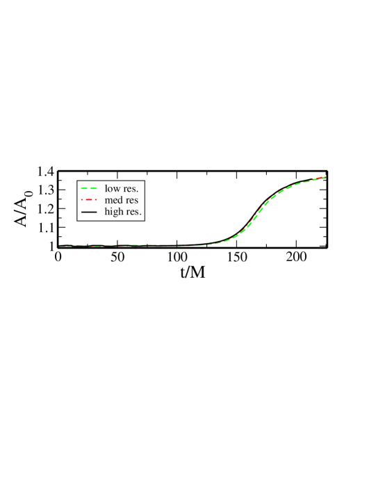
Figure 1: Apparent horizon area as a function of time for the perturbed black string. What is shown is the area normalized to the initial area, and from simulations with 3 different resolutions (see the text for a description of the resolutions).

More insight into the dynamics of the horizon can be garnered by observing the evolution of its intrinsic geometry with time. Fig. 2 shows several snapshots of embedding diagrams of the AH, from the medium resolution simulation run. As can be seen in the figure, the string initially evolves to a configuration resembling a hyperspherical black hole connected by a thin string segment, as reported earlier in (Choptuik et al.,, 2003, where the simulation ended at roughly $t\sim 164M$). However, as the evolution proceeds it is apparent that the string segments are themselves unstable, and this pattern repeats in a self-similar manner to ever smaller scales.

Though the intrinsic geometry on the horizon resembles spheres connected by strings, this by itself does not imply the local spacetime geometry is similar to either 5D spherical black holes or black strings, respectively. However, evaluation of the curvature invariants (24) on the horizon gives further insight into this question, and this is shown in Fig. 3, taken from the last time step of the medium resolution run. As seen in the figure, near spherical-like sections the normalized invariants approach $6$, in contrast to the string-like sections where they are close to $1$; thus, at least based on these two invariant indicators, the near horizon geometry indeed resembles that of the solutions suggested by the shape of the AH.

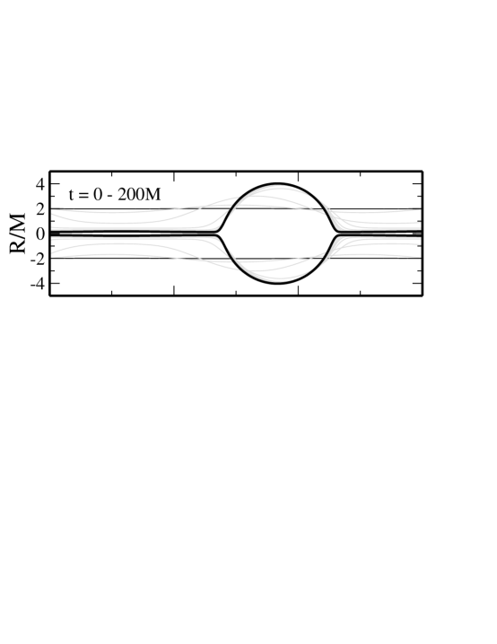
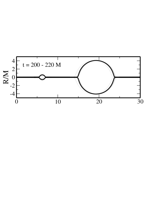
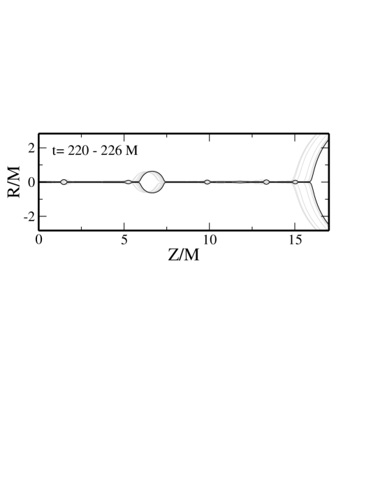
Figure 2: Embedding diagram of the apparent horizon at several instances in the evolution of the perturbed black string, from the medium resolution run. $R$ is areal radius, and the embedding coordinate $Z$ is defined so that the proper length of the horizon in the space-time $w$ direction (for a fixed $t,\theta,\phi$) is exactly equal to the Euclidean length of $R(Z)$ in the above figure. For visual aid copies of the diagrams reflected about $R=0$ have also been drawn in. In the top panel, the thin black lines are from the initial time; in the top two panels the thick black lines are the last time from the time-segment depicted in the corresponding panel, whereas in the bottom panel the last time-snapshot has been drawn with a thin black line. Note that the vertical and horizon axis scales have been changed in the bottom panel to better show the satellites that have formed at late times. The computational domain is periodic in $w$ with period $\delta w=20M$; at the initial (final stage of the simulation) $\delta Z=20M$, ($\delta Z=27.2M$)—see also Fig. 5

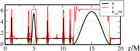
Figure 3: Curvature invariants evaluated on the apparent horizon at the last time of the medium resolution simulation (as depicted in Fig. 2). Also, for visual aid, the areal radius of the apparent horizon is shown. The invariant $K$ evaluates to $1$ for an exact black string, and $6$ for an exact spherical black hole; similarly for $S$ (24).

2 Interpretation of the horizon dynamics

The shape of the AH in the embedding diagram, and that the invariants are tending to the limits associated with pure black strings or black holes at corresponding locations on the AH, suggests it is reasonable to describe the local geometry as being similar to a sequence of black holes connected by black strings. This also strongly suggests that satellite formation will continue in a self-similar cascade, as each string segment locally resembles a rather uniform black string, and is sufficiently thin and long to be unstable. Note that even if at some point in the cascade thick segments were to form, this would generically not be a stable configuration, as (except possibly in an exactly symmetric situation) the satellites will have some non-zero $w$-velocity; hence they would eventually merge, effectively lengthening the segments connecting the remaining satellites.

With this interpretation, we can understand key features of the AH dynamics by sequencing its time evolution into generations of satellite formation. We assign a time $t_{i}$ to the onset of a new generation when the local instability has reached an “observable” level, defined here (somewhat arbitrarily) as the time when a nascent spherical region reaches an areal radius $1.5$ times the surrounding string radius. For each generation we measure the number $n_{s}$ of satellite black holes that form per string-segment, their radii $R_{AH,i}$ as well as the corresponding string segment’s radii $R_{s,i}$ and lengths $L_{s,i}$. These features are summarized in Table 1, where error bars, where appropriate, come from convergence calculations. Only the first generation is in a sense non-generic, as, by construction, only one unstable mode is initially allowed to develop. Generations after the first one display string segments where their ratio $L_{s,i}/R_{s,i}\simeq 100$ is not only above the critical one ($\simeq 7.2$), but can in principle accommodate several unstable modes (though see the discussion in Sec. 1). One would expect the mode closest to the maximum in the dispersion relation to dominate in each segment, and thus qualitatively similar dynamics to unfold from one generation to the next. In particular, we see that the time scale for the development of the $n^{th}$ generation of the instability is essentially the same along each string segment, as are the radii of the corresponding strings and spheres that form. However, beyond the second generation we find variation in the number $n_{s}$ of satellites that form as a function of resolution (hence the $\geq 1$ in the table). This suggests that exactly which mode dominates depends sensitively on the initial conditions, sufficiently so that a small perturbation, here coming from numerical truncation error, can change the quantitative details of the late time dynamics. This is not unexpected, as from the Gregory-Laflamme dispersion relation, except for the mode exactly at the maximum, there are two unstable modes with the same growth rate.

Gen.	$t_{i}/M$	$n_{s}$	$R_{s,i}/M$	$R_{AH,f}/M$	$L_{s,i}/R_{s,i}$
1	$118.1\pm 0.5$	$1$	$2.00$	$4.09\pm 0.5\%$	$10.0$
2	$203.1\pm 0.5$	$1$	$0.148\pm 1\%$	$0.63\pm 2\%$	$105\pm 1\%$
3	$223\pm 2$	$\geq 1$	$0.05\pm 20\%$	$0.1-0.2$	$\approx 10^{2}$
4	$\approx 227$	$\geq 1$	$\approx 0.02$	?	$\approx 10^{2}$

Table 1: Properties of the black string apparent horizon (see the text for a discussion).

Extrapolation to the end-state

The above observation of solution properties allow us to extrapolate to the end-state of the instability, estimating the time when this will occur, and the structure of the horizon just prior to it. We first calculate when the self-similar cascade will end, namely, the time when the connecting string segments reach zero radius, and then estimate the fractal dimension of the AH geometry just prior to this end.

The time when the first generation satellite appears is controlled by the perturbation imparted by the initial data, which here is $T_{0}/M\approx 118$. Subsequent generations, however should represent the generic development of the instability. From the data in the table, the time of growth of the first instability beyond the one sourced by the initial data is $T_{1}/M\approx 80$. Beyond that, with the caveats that we have a small number of data points and poor control over the error at late times, the data suggests each subsequent instability unfolds on a time-scale $X\approx 1/4$ times that of the preceding one. Again this is to be expected if the instability is qualitatively like the Gregory-Laflamme instability of the exact black string, where the time scale is proportional to the string radius. Then, the total time $\Delta T$ for the end-state to be reached is roughly

$$\Delta T\approx T_{0}+\sum_{i=0}^{\infty}T_{1}X^{i}=T_{0}+\frac{T_{1}}{1-X}.$$ (25)

For this case then, $\Delta T/M\approx 231$. At this time all string segments will reach zero radius. Since the Kretchman curvature invariant (24) just outside a string segment of radius $r$ is proportional to $r^{-4}$, and recalling that here (harmonic) time is regular everywhere from some distance inside the AH outwards and corresponds to the time measured by stationary asymptotic observers, this indicates formation of a naked singularity, and thus a violation of cosmic censorship. Furthermore, it is generic in the sense that no fine-tuning of the initial data is required (i.e., any length-wise perturbation exceeding the critical wavelength will do).

To give further evidence that the data supports the above conclusion, in Fig. 4 we show the time evolution of the radius of several representative cross-sections of the AH, in logarithmic coordinates where time has been shifted by the estimated time of naked singularity formation. That the radius of string-like segments decrease linearly in shifted-logarithmic time is consistent with a self-similar scaling to zero radius at the corresponding finite asymptotic time. Another intriguing aspect of this self-similar scaling is that it is qualitatively the same as that observed in the approach to pinch-off of Raleigh-Plateau unstable fluid streams. In the fluid case, a scaling solution is known (Eggers,, 1993; Miyamoto,, 2010), and the radius $R$ of the fluid column decreases linearly with time $t$ to fluid breakup $t=t_{c}$:

$$R\propto(t_{c}-t).$$ (26)

Fig. 4 shows that this, to good approximation, also describes shrinking regions of the black string.

A further consequence of the self-similar nature of the instability is that the AH shape will develop a fractal structure prior to pinch-off. This implies that for a fixed angular cross section ($\theta,\phi={\rm const.}$) of the horizon, the proper length $L_{p}(t)$ (within the periodically identified domain) will grow with each subsequent generation, diverging at a rate related to the Hausdorff dimension $d$ of the end-state shape. Assuming a scaling relation of the form (26), that the additional length in each new generation is caused by every string segment developing (on average) the same number $n_{s}$ of satellites, each with radii $R_{AH,f}$ following the scaling suggested in Table 1, and that $n_{s}\times R_{AH,f}/L_{s,i}\ll 1$, one can show that the following growth of $L_{p}(t)$ is expected

$$L_{p}(t)\propto(t_{c}-t)^{(1-d)}.$$ (27)

Figure 5 shows a plot of $L_{p}(t)$ on a logarithmic scale. From the measured slope and above relationship, we find $d\simeq 1.05$, which as expected is greater than a value of $1$ (that would correspond to a non-fractal curve) but only slightly, as the fractal structure is obtained by repeatedly replacing a relatively long straight line with a similar length line plus a small semi-circular protrusion.

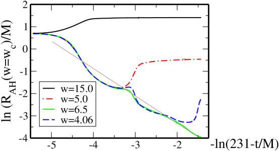
Figure 4: Logarithm of the areal radius vs. logarithm of time for select points on the apparent horizon, from the same (medium) resolution run depicted in Fig. 2. We have shifted the time axis assuming self-similar behavior; the putative naked singularity forms at asymptotic time $t/M\approx 231$. The coordinates at $w=15,5$ and $4.06$ correspond to the maxima of the areal radii of the first and second generation satellites, and one of the third generation satellites at the time the simulation stopped (the $w$ positions of the satellites do slightly evolve with time). The value $w=6.5$ is a representative slice that is in the middle of a piece of the horizon that remains string-like throughout the evolution. For visual aid in comparison with the analogue fluid pinch-off scaling solution (26), a line with slope equal to -1 has been added (thin brown line).

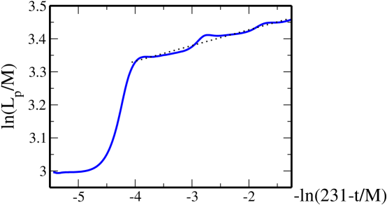
Figure 5: The proper length $L_{p}(t)$ vs. time of the apparent horizon in logarithmic coordinates, along a fixed azimuthal cross-section ($\theta=\phi=$ constant in spherical coordinates) and over one period of the spacetime in the $w$ direction. The time coordinate is scaled as in Fig.4. The dotted line is a visual linear fit to the late-time dynamics, and has a slope of $\sim 0.048$.

5 Speculations and Open Questions

In this chapter we described the evolution of an unstable black string in 5D, at least as far as was numerically feasible given finite computational resources, and extrapolated the observed behavior to describe the nature of the end-state of the instability. This has provided a first insight into the fascinating dynamics of unstable horizons in higher dimensions, yet has raised many questions and opened up avenues for future work. In this section we conclude by discussing in Sec. 1 whether the Gregory-Laflamme linear perturbative analysis can be used to quantitatively understand the dynamics of subsequent generations of the string instability, in Sec. 2 mention when quantum corrections are expected to become important as the string thins, and end with a list of open questions for future directions in Sec. 3.

1 Mode behavior

To gain more insight into what determines the observed dynamical behavior, we analyze the different modes in a string segment at the late stages of the first generation shown in Table 1, corresponding to the early stages of the growth of the second generation. In particular, we look at $R_{AH}(t,w)$ in $t\in(175M,205M)$ when only one spherical region is clearly distinguishable, and, in our coordinates this region has extent in $w\in[10,20M]$. The string section corresponds to $w\in[0,10M]$, and we decompose $R_{AH}(t,w)$ in this latter domain via the following expansion

$$R_{AH}(t,w)=c_{0}-\Sigma_{l=1}^{\infty}c_{l}\sin(l\pi w)\,,$$ (28)

and extract the coefficients $c_{l}$ up to $l=6$. Figure 6 illustrates the values $c_{l}/c_{0}$ within this time frame, and we only plot the odd values of $l$ as $\{c_{2},c_{4},c_{6}\}$ are about two orders of magnitude smaller. This is consistent with the observed symmetry in the development of the single second generation hypersphere within this segment, as it forms exactly in the middle of the string. Interestingly, of the odd modes, only $l=1$ displays growing behavior even though the length/radius ratio of the string at this time would allow for several modes to be unstable according to the Gregory-Laflamme instability criteria. This may not be too surprising however, as during this stage the solution is highly dynamical, shrinking in radius at a rate comparable to that at which putative Gregory-Laflamme modes could grow. This suggests that the linear analysis perturbing about the static black string “background” is not applicable here, and can only capture the qualitative nature of subsequent generations of instability. Note though that this is not in tension with the observation provided by the invariants $K$ and $S$, as the string can shrink in a time-dependent fashion and still maintain $K\approx S~{}\approx 1$.

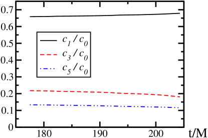
Figure 6: Vales of expansion coefficients for the string segment corresponding to the first generation. Even modes (except $c_{0}$) are a few orders of magnitude smaller than odd modes.

2 Dynamics Beyond the Classical Regime

As discussed, our classical description of the system reveals cascading self-similar behavior of the horizon, with regions evolving to ever shrinking cross-sectional radius. Such regions asymptote (in finite time) to a zero-mass naked singularity. Obviously for small enough regions, a classical description is no longer applicable and quantum phenomena must be taken into account. This is typically expected to happen when the cross-sectional radius $r$ approaches some small length $\ell$ scale (e.g. the Planck length $l_{p}$ or the string length $l_{s}$), though exactly when depends on the details of the leading order corrections to the field equations. For example, stringy-corrections predict this to be of the form

$$R_{\mu\nu}=\ell^{2}R_{\mu\alpha\beta\gamma}R_{\mu}{}^{\alpha\beta\gamma}+\cdots.$$ (29)

Since each term in (29) has dimension 1/length², a naive estimate of when the RHS becomes important is when its magnitude becomes of order $1/r^{2}$, as $r$ is the relevant length scale in the vicinity of a shrinking region of the horizon. Since $R_{\mu\alpha\beta\gamma}\sim 1/r^{2}$ there, this suggests corrections to general relativity are important when $\ell^{2}/r^{4}\sim 1/r^{2}$; i.e. if $\ell=l_{p}$, when the radius shrinks to the Planck length.

Another effect that could in principle alter the classical picture before the Planck scale is reached is if the timescale of Hawking evaporation $\tau_{H}$ of the string segment becomes smaller than the Gregory-Laflamme timescale $\tau_{GL}$. However, as the following shows, $\tau_{H}$ only becomes smaller than $\tau_{GL}$ beyond the Planck scale.

Assuming that a 4D description of evaporation at a $w={\rm const.}$ cross section of a string-like region gives a decent approximation to an evaporating string, we can estimate the timescale of Hawking evaporation and compare it to the timescale for development of the next generation within the self-similar cascade. From the simulation results, we have roughly that

$$\tau_{GL}\simeq 100M_{i}G/c^{3},$$ (30)

while that for Hawking evaporation of a 4D black hole of mass $M_{i}$ is

$$\tau_{H}=10240\pi^{2}\left(\frac{c^{5}}{hG}\right)\left(\frac{GM_{i}}{c^{3}}\right)^{3}.$$ (31)

Thus, for these two times to become comparable

$$M_{i}\simeq 10^{-1}\sqrt{\frac{\hbar c}{G}}=10^{-1}M_{P},$$ (32)

where $M_{P}$ is the Planck mass. This suggests that if the length scale $\ell$ in (29) is of order the Planck length or larger, then higher curvature corrections will generically be more important in describing the leading order alterations to the classical description of the instability than Hawking evaporation.

3 Future work

We conclude this chapter by listing some open questions and directions for future work, though this is by no means an exhaustive list.

First, consider a broader class of initial perturbations of the 5D black string where other unstable modes, and possibly linear combinations of modes with similar growth rates, are exited. We do not expect anything to change in a radical fashion, as the qualitative nature of the linear growth of all these modes is similar. Nevertheless, a quantitative analysis of such scenarios would tell if this expectation bares out, and allow one to understand how (if at all) the initial perturbation affects the unfolding structure of subsequent generations of the instability. On a similar vein, exploring how adding angular momentum to the string changes the picture would be interesting. Again the qualitative picture should not change, since as argued in Emparan et al., 2010, and shown at the linear level in Dias et al., 2010, rotation does not suppress the instability. However in Marolf and Palmer, 2004 it was suggested that rotation could induce super-radiant and gyrating instabilities; this should make for much richer dynamics in the approach to the end-state. Allowing for angular momentum would require less symmetry, making for more expensive numerical evolution.

Second, extract more details about the spacetime, such as the evolution of the generators of the horizon (as in Garfinkle et al.,, 2005), and the gravitational waves that are emitted as the instability unfolds. Perhaps the most profound question raised by these results is the striking qualitative similarity between the non-linear evolution of the instability and the Rayleigh-Plateau instability. Is this a coincidence, or the consequence of a deeper relationship between Einstein and Navier-Stokes than already suggested by the membrane paradigm, black folds and other perturbative descriptions of horizon dynamics? What would be useful in trying to understand this is to identify and extract geometric characteristics of the dynamical horizon that would map to effective fluid properties. Such a map could also prove useful in taking what is known about the Rayleigh-Plateau instability to learn more about Gregory-Laflamme; for example, translating the Eggers scaling solution (Eggers,, 1993) to an approximate solution for a thinning string segment.

Third, consider non-vacuum spacetimes; in particular charged black strings would be interesting as charges modify the onset of instabilities in the system  (for e.g. Gregory and Laflamme,, 1994; Sarbach and Lehner,, 2005).

Fourth, study a case where the spacetime is asymptotically flat in all spatial directions (the current study imposed periodicity in the fifth dimension). This would be required to provide an example of cosmic censorship violation in the 5D asymptotically flat case. However, it is natural to expect the same behavior as seen here based on the following putative scenario. Begin with a highly distorted $S^{3}$ horizon, namely one which is long and thin (“cigar shaped”) so that near the center of the horizon it locally resembles an $S^{2}\times R$ black string. One may expect that this horizon would ring-down via gravitational wave emission to a uniform $S^{3}$ horizon; however, if the dynamical time-scale for the ring-down (which will be proportional to the light-crossing time in the prolate direction, so could be made arbitrarily long) is much longer that the Gregory-Laflamme instability of the central region, then the latter should take over first, resulting in a pinch-off.

Fifth, explore black strings in higher dimensional spacetimes, particularly to investigate the conjecture of (Sorkin,, 2004) that a qualitatively different end-state is expected for $D>13$. If one continues to impose $SO(D-2)$ symmetry the problem can still be expressed to depend only on $(t,r,w)$, making it tractable with current computational resources. However, as the fields decay as $\{r^{D-3},r^{D-2}\}$ moving away from black hole, black string solutions respectively, the resolution and/or order of the numerical scheme would need to be higher than the one used in this work to obtain results of comparable accuracy.

Sixth, explore additional black objects subject to Gregory-Laflamme-like instabilities. For instance, rapidly rotating black holes have been shown to be subject to a similar instability (Emparan and Myers,, 2003). Recent numerical work presented the first exploration of such systems (Shibata and Yoshino,, 2010), though there radiation of angular momentum stabilizes the black holes considered. However, the growth rate of the instability in the cases studied was rather mild, and it is quite likely that choosing a more extreme scenario (where the timescale of the unstable modes would be shorter than the dynamical time of gravitational radiation) would give rise to a pinch-off similar to the one studied here.

Finally, evolve unstable black strings (and other black objects) within asymptotically Anti de Sitter (AdS) spacetime, and explore the consequences within the context of the AdS/Conformal Field Theory (CFT) dualities of string theory. This is partly related to the point mentioned above about further investigating the intriguing connections between gravity and fluids, as certain states within a CFT will admit a hydrodynamic description. Though regardless, understanding the CFT-duals to unstable black hole spacetimes is interesting in its own right, and could have implications to the more recent applications of AdS/CFT to model certain condensed matter and high energy particle physics systems.

6 Acknowledgements

We thank A. Buchel, V. Cardoso, M. Choptuik, R. Emparan, D. Garfinkle, K. Lake, S. Gubser, G. Horowitz, D. Marolf, R. Myers, E. Poison, W. Unruh and R. Wald for stimulating discussions. This work was supported by NSERC (LL), CIFAR (LL), the Alfred P. Sloan Foundation (FP), and NSF grant PHY-0745779 (FP). Research at Perimeter Institute is supported through Industry Canada and by the Province of Ontario through the Ministry of Research & Innovation.

References

- Alcubierre, (2008) Alcubierre, Miguel. 2008. Introduction to 3+1 Numerical Relativity. Oxford: Oxford Science Publications.
- Alcubierre et al., (2001) Alcubierre, Miguel, Brandt, Steven, Bruegmann, Bernd, Holz, Daniel, Seidel, Edward, et al. 2001. Symmetry without symmetry: Numerical simulation of axisymmetric systems using Cartesian grids. Int.J.Mod.Phys., D10, 273–290.
- Anderson et al., (2006) Anderson, Matthew, Lehner, Luis, and Pullin, Jorge. 2006. Arbitrary black-string deformations in the black string - black hole transitions. Phys. Rev., D73, 064011.
- Baumgarte and Shapiro, (2010) Baumgarte, Thomas W., and Shapiro, Stuart L. 2010. Numerical Relativity : Solving Einstein’s Equations on theComputer. Camdridge: Cambridge Universtity Press.
- Berger and Oliger, (1984) Berger, Marsha J., and Oliger, Joseph. 1984. Adaptive Mesh Refinement for Hyperbolic Partial Differential Equations. J.Comput.Phys., 53, 484.
- Bhattacharyya et al., (2008) Bhattacharyya, Sayantani, Hubeny, Veronika E, Minwalla, Shiraz, and Rangamani, Mukund. 2008. Nonlinear Fluid Dynamics from Gravity. JHEP, 0802, 045.
- Bona and Palenzuela-Luque, (2005) Bona, Carles, and Palenzuela-Luque, Carlos. 2005. Elements of Numerical Relativity. Berlin: Springer-Verlag.
- Buchel and Liu, (2004) Buchel, Alex, and Liu, James T. 2004. Universality of the shear viscosity in supergravity. Phys. Rev. Lett., 93, 090602.
- Calabrese et al., (2004) Calabrese, Gioel, Lehner, Luis, Reula, Oscar, Sarbach, Olivier, and Tiglio, Manuel. 2004. Summation by parts and dissipation for domains with excised regions. Class.Quant.Grav., 21, 5735–5758.
- Camps et al., (2010) Camps, Joan, Emparan, Roberto, and Haddad, Nidal. 2010. Black Brane Viscosity and the Gregory-Laflamme Instability. JHEP, 1005, 042.
- Cardoso and Dias, (2006) Cardoso, Vitor, and Dias, Oscar J. C. 2006. Gregory-Laflamme and Rayleigh-Plateau instabilities. Phys. Rev. Lett., 96, 181601.
- Choptuik et al., (2003) Choptuik, Matthew W., Lehner, Luis, Olabarrieta, Ignacio, Petryk, Roman, Pretorius, Frans, et al. 2003. Towards the final fate of an unstable black string. Phys.Rev., D68, 044001.
- Dias et al., (2010) Dias, Oscar J.C., Figueras, Pau, Monteiro, Ricardo, Reall, Harvey S., and Santos, Jorge E. 2010. An instability of higher-dimensional rotating black holes. JHEP, 1005, 076.
- Eggers, (1993) Eggers, J. 1993. Universal pinching of 3D axisymmetric free-surface flow. Physical Review Letters, 71(Nov.), 3458–3460.
- Eggers, (1997) Eggers, Jens. 1997. Nonlinear dynamics and breakup of free-surface flows. Rev.Mod.Phys., 69, 865–930.
- Emparan and Myers, (2003) Emparan, Roberto, and Myers, Robert C. 2003. Instability of ultra-spinning black holes. JHEP, 09, 025.
- Emparan et al., (2009) Emparan, Roberto, Harmark, Troels, Niarchos, Vasilis, and Obers, Niels A. 2009. World-Volume Effective Theory for Higher-Dimensional Black Holes. Phys.Rev.Lett., 102, 191301.
- Emparan et al., (2010) Emparan, Roberto, Harmark, Troels, Niarchos, Vasilis, and Obers, Niels A. 2010. Essentials of Blackfold Dynamics. JHEP, 1003, 063.
- Friedrich, (1985) Friedrich, H. 1985. On the hyperbolicity of Einstein’s and other gauge field equations. Communications in Mathematical Physics, 100(Dec.), 525–543.
- Garfinkle, (2002) Garfinkle, David. 2002. Harmonic coordinate method for simulating generic singularities. Phys. Rev., D65, 044029.
- Garfinkle et al., (2005) Garfinkle, David, Lehner, Luis, and Pretorius, Frans. 2005. A numerical examination of an evolving black string horizon. Phys. Rev., D71, 064009.
- Gregory and Laflamme, (1993) Gregory, R., and Laflamme, R. 1993. Black strings and p-branes are unstable. Phys.Rev.Lett., 70, 2837–2840.
- Gregory and Laflamme, (1994) Gregory, Ruth, and Laflamme, Raymond. 1994. The Instability of charged black strings and p-branes. Nucl.Phys., B428, 399–434.
- Gubser, (2002) Gubser, Steven S. 2002. On non-uniform black branes. Class. Quant. Grav., 19, 4825–4844.
- Gundlach et al., (2005) Gundlach, Carsten, Martin-Garcia, Jose M., Calabrese, Gioel, and Hinder, Ian. 2005. Constraint damping in the Z4 formulation and harmonic gauge. Class.Quant.Grav., 22, 3767–3774.
- Guzman et al., (2007) Guzman, F. S., Lehner, L., and Sarbach, O. 2007. Do unbounded bubbles ultimately become fenced inside a black hole? Phys. Rev., D76, 066003.
- Hawking and Ellis, (1973) Hawking, S.W., and Ellis, G.F.R. 1973. The Large scale structure of space-time.
- Horowitz and Maeda, (2001) Horowitz, Gary T., and Maeda, Kengo. 2001. Fate of the black string instability. Phys. Rev. Lett., 87, 131301.
- Hovdebo and Myers, (2006) Hovdebo, J. L., and Myers, Robert C. 2006. Black rings, boosted strings and Gregory-Laflamme. Phys. Rev., D73, 084013.
- Kol, (2006) Kol, Barak. 2006. The Phase Transition between Caged Black Holes and Black Strings - A Review. Phys. Rept., 422, 119–165.
- Kol and Wiseman, (2003) Kol, Barak, and Wiseman, Toby. 2003. Evidence that highly non-uniform black strings have a conical waist. Class. Quant. Grav., 20, 3493–3504.
- Kovtun et al., (2005) Kovtun, P., Son, D. T., and Starinets, A. O. 2005. Viscosity in strongly interacting quantum field theories from black hole physics. Phys. Rev. Lett., 94, 111601.
- Kudoh and Wiseman, (2004) Kudoh, Hideaki, and Wiseman, Toby. 2004. Properties of Kaluza-Klein black holes. Prog. Theor. Phys., 111, 475–507.
- Lehner and Pretorius, (2010) Lehner, Luis, and Pretorius, Frans. 2010. Black Strings, Low Viscosity Fluids, and Violation of Cosmic Censorship. Phys.Rev.Lett., 105, 101102.
- Lindblom et al., (2006) Lindblom, Lee, Scheel, Mark A., Kidder, Lawrence E., Owen, Robert, and Rinne, Oliver. 2006. A New generalized harmonic evolution system. Class.Quant.Grav., 23, S447–S462.
- Marolf, (2005) Marolf, Donald. 2005. On the fate of black string instabilities: An observation. Phys. Rev., D71, 127504.
- Marolf and Palmer, (2004) Marolf, Donald, and Palmer, Belkis Cabrera. 2004. Gyrating strings: A New instability of black strings? Phys.Rev., D70, 084045.
- Miyamoto, (2010) Miyamoto, Umpei. 2010. One-Dimensional Approximation of Viscous Flows. JHEP, 10, 011.
- Okawa et al., (2011) Okawa, Hirotada, Nakao, Ken-ichi, and Shibata, Masaru. 2011. Is super-Planckian physics visible? – Scattering of black holes in 5 dimensions.
- Palenzuela et al., (2009) Palenzuela, Carlos, Anderson, Matthew, Lehner, Luis, Liebling, Steven L., and Neilsen, David. 2009. Stirring, not shaking: binary black holes’ effects on electromagnetic fields. Phys. Rev. Lett., 103, 081101.
- Pretorius, (2005a) Pretorius, Frans. 2005a. Evolution of binary black hole spacetimes. Phys.Rev.Lett., 95, 121101.
- Pretorius, (2005b) Pretorius, Frans. 2005b. Numerical relativity using a generalized harmonic decomposition. Class.Quant.Grav., 22, 425–452.
- Pretorius, (2007) Pretorius, Frans. 2007. Binary Black Hole Coalescence.
- Price, (1972) Price, R. H. 1972. Nonspherical Perturbations of Relativistic Gravitational Collapse. I. Scalar and Gravitational Perturbations. Phys.Rev.D., 5(May), 2419–2438.
- Sarbach and Lehner, (2004) Sarbach, Olivier, and Lehner, Luis. 2004. No naked singularities in homogeneous, spherically symmetric bubble spacetimes? Phys. Rev., D69, 021901.
- Sarbach and Lehner, (2005) Sarbach, Olivier, and Lehner, Luis. 2005. Critical bubbles and implications for critical black strings. Phys. Rev., D71, 026002.
- Shibata and Yoshino, (2010) Shibata, Masaru, and Yoshino, Hirotaka. 2010. Bar-mode instability of rapidly spinning black hole in higher dimensions: Numerical simulation in general relativity. Phys. Rev., D81, 104035.
- Sorkin, (2004) Sorkin, Evgeny. 2004. A critical dimension in the black-string phase transition. Phys. Rev. Lett., 93, 031601.
- Sorkin and Choptuik, (2010) Sorkin, Evgeny, and Choptuik, Matthew W. 2010. Generalized harmonic formulation in spherical symmetry. Gen.Rel.Grav., 42, 1239–1286.
- Sorkin and Piran, (2003) Sorkin, Evgeny, and Piran, Tsvi. 2003. Initial data for black holes and black strings in 5d. Phys. Rev. Lett., 90, 171301.
- Szilagyi and Winicour, (2003) Szilagyi, Bela, and Winicour, Jeffrey. 2003. Well-Posed Initial-Boundary Evolution in General Relativity. Phys. Rev., D68, 041501.
- Thornburg, (2007) Thornburg, Jonathan. 2007. Event and apparent horizon finders for 3+1 numerical relativity. Living Rev.Rel., 10, 3.
- Thorne et al., (1986) Thorne, Kip S., (Ed.), Price, R.H., (Ed.), and Macdonald, D.A., (Ed.). 1986. BLACK HOLES: THE MEMBRANE PARADIGM.
- Wiseman, (2003) Wiseman, Toby. 2003. Static axisymmetric vacuum solutions and non-uniform black strings. Class. Quant. Grav., 20, 1137–1176.
- Witek et al., (2010) Witek, Helvi, et al. 2010. Black holes in a box: towards the numerical evolution of black holes in AdS. Phys. Rev., D82, 104037.
- Witek et al., (2011) Witek, Helvi, et al. 2011. Head-on collisions of unequal mass black holes in D=5 dimensions. Phys. Rev., D83, 044017.