Using a Differential Emission Measure and Density Measurements in an Active Region Core to Test a Steady Heating Model

Abstract

The frequency of heating events in the corona is an important constraint on the coronal heating mechanisms. Observations indicate that the intensities and velocities measured in active region cores are effectively steady, suggesting that heating events occur rapidly enough to keep high temperature active region loops close to equilibrium. In this paper, we couple observations of Active Region 10955 made with XRT and EIS on Hinode to test a simple steady heating model. First we calculate the differential emission measure of the apex region of the loops in the active region core. We find the DEM to be broad and peaked around 3 MK. We then determine the densities in the corresponding footpoint regions. Using potential field extrapolations to approximate the loop lengths and the density-sensitive line ratios to infer the magnitude of the heating, we build a steady heating model for the active region core and find that we can match the general properties of the observed DEM for the temperature range of 6.3 $<$ Log T $<$ 6.7. This model, for the first time, accounts for the base pressure, loop length, and distribution of apex temperatures of the core loops. We find that the density-sensitive spectral line intensities and the bulk of the hot emission in the active region core are consistent with steady heating. We also find, however, that the steady heating model cannot address the emission observed at lower temperatures. This emission may be due to foreground or background structures, or may indicate that the heating in the core is more complicated. Different heating scenarios must be tested to determine if they have the same level of agreement.

1 Introduction

A major problem in coronal physics is to determine the mechanisms that transfer and dissipate energy that heat the million-degree corona. Regardless of the transfer or dissipation mechanism, the predicted timescale for energy release for all mechanisms is finite, i.e., a single heating event is relatively short-lived (Klimchuk, 2006). The frequency of heating events occurring on a single strand in the corona, however, could distinguish between the different theoretical mechanisms. (Here, we use the term “strand” to refer to the fundamental flux tube in the corona, and the term “loop” to refer to a discernable structure in an observation. A loop could be formed of a single strand, which would imply we are currently resolving the corona, or it could be formed of many, sub-resolution strands.)

There has been significant debate as to whether observations support high- or low-frequency heating. If heating events that occur on a single strand are frequent (i.e., the time between individual heating events is much shorter than the cooling time of the plasma) and approximately uniform, then the temperature and density of the plasma along the strand are effectively steady as the plasma does not have time to cool or drain between heating events. Such a heating scenario predicts a loop with steady intensities and velocities. If the heating events are infrequent (i.e., the time between heating events is much longer than the cooling time of the plasma), then the resulting temperature and density of the plasma along the strand will evolve; such a heating scenario is often termed “nanoflare heating” (e.g., Cargill & Klimchuk, 1997), though it could be representative of different types of mechanisms, not simply Parker’s canonical nanoflare theory (Parker, 1972). The evolution of the plasma may or may not be apparent in loop observations depending on the number of strands the make up the loop and the relative timing of their heating events. In the case of a loop formed of only a few strands that undergo a burst of heating events close in time, the observed loop’s properties, such as the intensity of the loop in a spectral line or filter, would appear to evolve as the strands evolve (Warren et al., 2002); such a heating scenario is sometimes called a “short nanoflare storm” (Klimchuk, 2009). If the loop is formed of many sub-resolution strands, each strand being heated and evolving randomly, then the observed loop’s intensity would appear steady regardless of the dynamic nature of the plasma along a single strand; this type of low-frequency heating is sometimes called a “long nanoflare storm” (Klimchuk, 2009).

Observations in active regions show both evolving and steady structures (Reale, 2010). So-called “warm,” 1 MK loops that form a bright arcade in EUV images are evolving and their properties are consistent with low-frequency heating in the form of short-nanoflare storms (Winebarger et al., 2003; Warren et al., 2003; Winebarger & Warren, 2005; Ugarte-Urra et al., 2006, 2009; Mulu-Moore et al., 2011). The intensities of the hot ($>$ 2 MK) loops that make up the active region cores, however, appear to be steady over many hours of observation (e.g., Warren et al., 2010, 2011). This steadiness is apparent in both the X-ray intensity over the neutral line and in the footpoints of the hot loops observed in the EUV and commonly called moss (e.g., Antiochos et al., 2003). Additionally, the velocities and non-thermal velocities in the moss are also steady for hours of observations (Brooks & Warren, 2009). The steadiness of the intensities and velocities has prompted many to hypothesize the heating in the core regions is effectively steady. However, different heating scenarios, such as the long nanoflare storm scenario described above, also predict steady intensities and velocities. Additional comparisons between observations and simulations are necessary to discern whether the active region core is consistent with effectively steady heating. Warren et al. (2011) demonstrated that the properties of the plasma along strands suffering effectively steady (high-frequency) heating can be well approximated by the steady heating solutions to the hydrodynamic equations. In this paper, we will determine whether observations of the loops that form the active region core are consistent with the predictions of steady solutions to the hydrodynamic equations.

If the density and temperature in a well-isolated and resolved loop was known, it would be possible to test whether the loop was heated steadily or not using the so-called Rosner-Tucker-Vaiana (RTV) scaling laws (Rosner et al. 1978, also see Serio et al. 1981). These scaling laws define a relationship between the apex temperature, $T_{\rm apex}$, base pressure, $p_{0}$, and loop half-length, $L$, for steady uniform heating, i.e., $T_{\rm apex}=1.4\times 10^{3}(p_{0}L)^{1/3}$. However, individual loops are very difficult to isolate in active region cores, and loops that appear to be resolved may themselves be formed of sub-resolution strands, hence such a direct comparison with model predictions is not possible.

Another method to test whether a heating scenario is viable is to forward model the active region or full Sun as ensembles of strands with either a steady or infrequent heating model and then compare simulated images from the model to the observed images. Several studies have been completed using this technique (Schrijver et al. 2004; Warren & Winebarger 2006, 2007; Lundquist et al. 2008). In these studies, the field lines from the potential magnetic field were used to approximate the global or active region structure. The heating rate was assumed to be a function of the magnetic field strength and loop length. Several different parameters were varied, such as the functional form of the heating, the degree in which the loops expanded, and the non-uniformity of the heating along the loop. These studies determined that to best match the X-ray observations of the active regions, the heating must be proportional to average magnetic field strength and inversely proportional to loop length, the loops must expand with height, and the heating along the loop must be near uniform. (Note that loop expansion contradicts the observation that loops have near constant cross sections along their lengths; Klimchuk 2000.) There are two significant shortcomings of these previous studies. First, most of the studies relied on matching the intensities in a single X-ray filter. Second, the EUV footpoint emission from the moss was poorly matched by the models; in general, the moss emission was too bright.

In an attempt to simultaneously match both the EUV moss emission and the apex X-ray emission in two filters, Winebarger et al. (2008) modeled an active region core as an ensemble of strands. Instead of assuming a functional form of the heating, however, they used the TRACE 171 Å intensity in the moss region to limit the steady heating rate. The TRACE 171 Å intensity is pressure sensitive given an unknown filling factor (Martens et al., 2000). In this study, a filling factor was assumed for the entire moss region, then the pressure was derived from the TRACE 171 Å image. For each strand, a heating rate was determined that would match the pressure; the expected intensities in the X-ray filter data was then calculated. This process was completed for several different assumed filling factors. The best agreement for the X-ray filter intensities was found for loops that expand inversely with the magnetic field strength and for a filling factor of 8%. This study was the first successful steady heating model to account for both the footpoint EUV emission and apex X-ray emission. The weakness of this study was the forced assumption of a single filling factor for the entire moss region.

In this paper, we will determine whether observations from Hinode XRT and EIS agree with a steady heating model of the active region core. We build upon the previous full models of active region cores with two key improvements. First, instead of comparing model intensities with observed intensities in one or two filter images, we compare a differential emission measure (DEM) from the model with a DEM calculated from a combination of XRT filter and EIS spectral line intensities. Second, we use two density sensitive spectral lines (Fe XII 186.880/195.119 Å) in the moss region to simultaneously constrain both the pressure in the core loops and the filling factor. As with the previous studies, we use potential field extrapolations to approximate the loop length and geometry, assume the loops expand with height and assume the energy is deposited uniformly along the loop. We determine that the DEM from the steady heating model well matches the DEM from observations around the peak temperature in the active region core (6.3 $<$ Log T $<$ 6.7), as well as the spectral line intensities in both the Fe XII 186.880 and 195.119 Å lines in the footpoints of the active region. However, the steady heating model does not reproduce the observed DEM in the “warm” temperature range (6.1 $<$ Log T $<$ 6.3). This warm emission could originate from the overlying arcade and not from the core loops, or it could indicate that the heating in the active region core is more complicated. These results provide, for the first time, evidence that the high temperature loops in the core of an active region and their footpoint pressure can be well represented by high-frequency heating. Different heating scenarios must be tested to determine if they have the same level of agreement.

2 Data

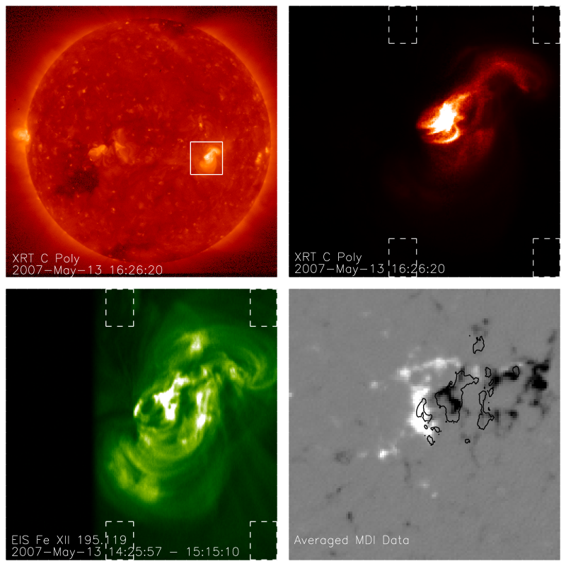
Figure 1: (Upper Left Panel:) Full disk image of the Sun in XRT C_poly filter scaled logarithmically. The box shows the EIS field of view. (Upper Right Panel:) A C_poly image (scaled linearly) in the EIS field of view. (Lower Left Panel:) The EIS Fe XII 195.119 Å raster of the active region. The squares made with dashed lines show the areas used for background subtraction. (Lower Right Panel:) The time average photospheric magnetic field measurements from MDI in the same field of view as the EIS data. The contours are from the Fe XII 186.880 Å raster.

Active Region 10955 was observed on 2007 May 13 by Hinode and Solar Heliospheric Observatory (SoHO) instruments. A full disk X-ray Telescope image is shown in Figure 1. The observations considered in this analysis were taken between 14:25 and 16:30 UT. At this time, the active region was approximately {445”,-149”} away from disk center.

The X-Ray Telescope (XRT; Golub et al. 2007) on Hinode (Kosugi et al., 2007) is a broadband instrument similar to the Yohkoh Soft X-Ray Telescope (Tsuneta et al., 1991), but with better spatial resolution, sensitivity, and temperature coverage. XRT has 1″pixels, 2″resolution, and 9 temperature sensitive filters that can be used alone or in combination. The XRT data used for this analysis were taken on 2007 May 13 from 16:17 - 16:30 UT. The data set is comprised of full Sun, full resolution images in multiple filters and filter combinations. The data processing included dark-frame subtraction, vignetting correction, and high-frequency noise removal using the standard xrt_prep routine available from SolarSoft. Spacecraft jitter was removed using xrt_jitter, and long and short exposures (see Table 1) were co-aligned and combined to increase the image dynamic range. Additional Fourier filtering was done to the data from the thickest channel, Be_thick, to remove low-level, residual, longer-wavelength noise patterns. We have used updated filter calibrations (Narukage et al. 2011) and accounted for a 1640-Å thickness of the time-dependent contamination layer on the CCD. (We used the “best-model” contaminant composition of diethylhexyl phthalate, as provided by the XRT calibration software, but we note that the true composition is as of yet undetermined.)

The EIS instrument on Hinode is a high spatial and spectral resolution imaging spectrograph. EIS observes two wavelength ranges, 171–212 Å and 245–291 Å, with a spectral resolution of about 22 mÅ and a spatial resolution of about 1″ per pixel. There are 1″ and 2″ slits as well as 40″ and 266″ slots available. Solar images can be made using one of the slots or by stepping one of the slits over a region of the Sun. Telemetry constraints generally limit the spatial and spectral coverage of an observation. See Culhane et al. (2007) and Korendyke et al. (2006) for more details on the EIS instrument.

In this analysis we consider EIS observations taken from 14:25:57 to 15:15:10 UT on 2007 May 13. For these observations the 1″ slit was stepped across the active region and a 10 s exposure was taken at each position. The area observed was $256\arcsec\times 256\arcsec$. A total of 16 data windows, some containing multiple emission lines, were downloaded from the spacecraft. The raw data was processed to remove the CCD pedestal, dark current, and spurious intensities from warm pixels. The pre-flight calibration was also applied to the data. Before the line profiles are fit it is necessary to correct for an oscillation in the EIS wavelength dispersion. We do this by assuming that there are no net velocity shifts along the bottom 30 pixels of the slit (see Brown et al. 2007 for details). For each emission line of interest the best-fit parameters for a single Gaussian were calculated.

The XRT and EIS data were aligned by cross correlating the Be_thin filter image from XRT with the Fe XVI 262.984 Å raster from EIS. The EIS field of view is shown in the XRT full disk image in Figure 1 as solid white lines. The entire EIS field of view for the C_poly filter and Fe XII 195.119 Å raster are also shown in Figure 1.

We use magnetic field measurements from the Michelson Doppler Imager (MDI) on SoHO. All of the 96-minute full disk magnetograms taken within 5 hours of the EIS data were aligned and averaged to reduce noise. The MDI magnetograms were aligned to the Fe XII 186.880 Å data. The averaged MDI data in the EIS field of view with the Fe XII 186.880 Å contours is shown in Figure 1.

3 Analysis

3.1 Differential Emission Measure

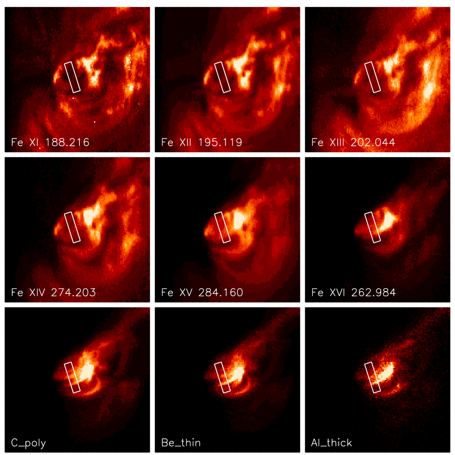
Figure 2: Several EIS rasters and XRT images from the data set. The solid lines indicate the region over which the intensity was averaged.

The first goal of this research is to determine the distribution of emission from the apex of the core loops. To complete this goal, a region between the moss in the core of the active region was selected. This region is shown in Figure 2 with solid lines in several example rasters or filter images. The emission in this region represents the intensity from the core of the active region plus ambient corona between the Sun and the telescope. To remove the ambient corona, we selected four background regions at the edge of the field of view, shown in Figure 1 as dashed lines. We average the intensity in the region of interest and subtract the average background intensity. The background-subtracted intensities are given in Table 2. EIS intensities are given in ergs cm^-2 s^-1 sr^-1 and XRT intensities are given in DN s^-1 pix^-1.

For this work we have included EIS observations of the Fe XVII line at 254.87 Å. This line is problematic for several reasons. Both the emissivity of this line and the effective area of EIS at this wavelength are relatively small, which makes the line difficult to observe. Furthermore, the atomic data for this transition appears to be inconsistent with the other Fe XVII and high temperature Ca lines observed with EIS Warren et al. (2008). These differences appear to be about a factor of 2. Since this is the highest temperature line observed with EIS outside of flares it is useful to accept these limitations so that we can have better overlap between the EIS and XRT observations.

The uncertainties in the EIS intensities given in Table 2 are the calculated statistical errors due to photon noise and the error in the Gaussian fits and an assumed 22% systematic error associated with the absolute calibration of the EIS data (Lang et al., 2006). The uncertainties in the XRT intensities due to photon noise are more difficult to assess. The method used to calculate the XRT errors in Table 2 is described below.

To generate possible DEM curves that can reproduce the observed fluxes given in Table 2, we have used xrt_dem_iterative2, which was designed originally for use with XRT data only but has been modified slightly to allow for inclusion of EIS data as well. Leading up to the launch of Hinode, Golub et al. (2004) and Weber et al. (2004) tested and validated the method with synthetic data. The routine employs a forward-fitting approach where a DEM is guessed and folded through each response to generate predicted fluxes. This process is iterated to reduce the $\chi^{2}$ between the predicted and observed fluxes. The DEM function is interpolated using several spline points, which are directly manipulated by mpfit, a well-known and much-tested IDL routine that performs a Levenberg-Marquardt least-squares minimization. This routine uses Monte-Carlo iterations to estimate errors on the DEM solution. For each iteration, the observed fluxes in each filter were varied randomly within the uncertainties and the program was run again with the new values.

The xrt_dem_interative2 program requires user input for the XRT response functions and EIS emissivity functions. The XRT filter responses were calculated using the XRT standard software (make_xrt_wave_resp and make_xrt_temp_resp). These programs account for the time dependent contamination of the XRT CCD. The EIS line emissivity functions were calculated using CHIANTI 6.0.1. The default abundances (Feldman et al. 1992) and ionization equilibrium (Mazzotta et al. 1998) were used. The emissivity functions for some ions are density sensitive. As a default, we find a density from the Fe XIII 202.044/203.826 Å intensity ratio. The ratio of the two background subtracted intensities given in Table 2 return a density of Log $n_{e}$ = 9.7 cm^-3. All emissivity functions were calculated using this density.

The data used in this analysis were taken on 2007 May 13, just before the first XRT CCD bake-out (2007 July 23). This bake-out was designed to remove the accumulating wavelength-dependent contamination layer that was affecting the instrument sensitivity. As a result, the contamination layer was close to maximum thickness. In addition, the XRT team was not yet taking regular G-band images, which is one of the tools used to estimate the thickness of the contamination layer. As a result, the thickness is not as well known. Al_mesh observations are generally the most affected by contamination, especially at low temperatures where the sensitivity is dependent mainly on longer wavelength spectral lines. In light of these uncertainties, and combined with the fact that we have EIS spectral lines that effectively cover the lower coronal temperatures, we have elected to eliminate Al_mesh from the DEM calculation.

XRT is a broadband instrument allowing photons of many different energies to generate electrons on the detector. The number of electrons that are generated are proportional to the photon energy, so there is no a priori way to deduce the number of photons that produced a signal from the number of electrons deposited onto the detector. The measured count rate in a pixel could be from a few high-energy photons or from many low-energy photons, and the uncertainty would vary accordingly. Below we describe how we use a “bootstrap” method to calculate the errors associated with photon uncertainties.

To determine the XRT filter errors due to photon noise, we first calculate a DEM using the method described above assuming a 20% error in the XRT filter intensities. We then use that DEM to calculate the emerging spectrum from the solar plasma, $I_{solar}(\lambda)$, in photons s^-1 cm^-2 sr^-1 Å^-1. We convolve the spectrum with the effective area for each filter and multiply by the resolution, wavelength bin size, and exposure time for each filter to find the spectrum in photons at the detector in a given filter, i.e.,

$$I_{det}(\lambda)=I_{solar}(\lambda)*EA_{filter}(\lambda)*\Delta\lambda*t_{exp}*C.$$ (1)

In the above equation, the effective area, $EA_{filter}$, is in cm² and is taken from the XRT program make_xrt_wave_resp, the $\Delta\lambda$ is the size of the wavelength bin in Å, $t_{exp}$ is the exposure time, and the factor, $C$, is the sterradians subtended by one XRT pixel. After calculating the photons that interact with the detector, we determine the photon noise by taking the square root of this intensity, $\sigma_{det}=\sqrt{I_{det}}$. The intensity in a given pixel in data number (DN) can then be found by

$$I_{DN}=\sum I_{det}(\lambda)*\frac{E(\lambda)}{\epsilon_{0}}\frac{1}{G}$$ (2)

where $E$ is the energy associated with an incoming photon, $E(\lambda)=hc/\lambda$, $\epsilon_{0}$ is the energy per electron on the detector (3.65 eV), and $G$ is the gain of the detector (59 electron DN^-1). We then propagate the photon noise through this step to determine the error in the intensity in DN. Note there are additional sources of statistical uncertainty in this calculation, but they are small compared to the photon noise. We determine the relative uncertainty due to photon noise in the XRT filters are $<$5% in the thinnest filters and $>100$% in the thickest filter. We combine this statistical uncertainty with an assumed 20% systematic uncertainty in the absolute calibration of the XRT intensities. The uncertainties given in Table 2 reflect this analysis.

After completing the XRT error analysis, a new DEM was calculated with the updated errors. The results from the DEM calculations are shown in the left panel of Figure 3. The solid thick line shows the best DEM calculated for input intensities. The DEM is broad with a peak at Log T = 6.5. The intensities calculated in each spectral line or filter for this DEM are given in Table 2. In general, the ratio of the observed to modeled intensity is close to 1 with two exceptions. The Fe XVII spectral line intensity is off by a factor of 2; this is likely due to poor atomic data and is consistent with the results in Warren et al. (2008). Additionally, the Be_thick intensity calculated from the DEM is roughly a factor of 3 higher than observed.

The dotted lines clustered around the solid thick line are DEMs calculated by varying the input intensities within the uncertainties and hence provide an estimate of the uncertainty of the DEM. Another way to assess the uncertainty in the DEM and determine the temperature regime where the DEM is well constrained is to calculate how much additional emission could be added to a single temperature bin without changing the modeled intensities in any spectral line or filter by more than the expected errors. This value is shown as a blue line in Figure 3. For instance, the DEM calculated for Log T = 7.0 MK is approximately $6\times 10^{14}$ cm^-5 K^-1. We determine we could increase the DEM to $2\times 10^{20}$ cm^-5 K^-1 (a factor of $3\times 10^{5}$) without changing the modeled intensities by more than the errors. This implies this temperature bin is not well constrained and emission could be in this temperature bin, but the spectral lines and filters we are using in this analysis are not sensitive to it. The ratio of this “maximum DEM” to the calculated DEM is less than 3.0 in the temperature range of 6.1 $\leq$ Log T $\leq$ 6.7; we consider this temperature range well constrained by the observations.

If we define the differential emission measure to be $\xi=n^{2}ds/dT$, we can write the intensity in a given spectral line or filter, $I_{\lambda}$, in terms of the emissivity function or filter response function, $\epsilon_{\lambda}(T,n)$, i.e.,

$$I_{\lambda} = \frac{1}{4\pi}\int\epsilon_{\lambda}(T,n)\xi dT$$ (3)

$$1 = \int\frac{\epsilon_{\lambda}(T,n)}{4\pi I_{\lambda}}\xi dT$$ (4)

$$1 = \int\frac{1}{\xi_{\rm loci}(T)}\xi dT$$ (5)

where we have introduced the emission measure loci function,

$$\xi_{\rm loci}(T)=\frac{4\pi I_{\lambda}}{\epsilon_{\lambda}(T,n)}$$ (6)

(Jordan et al., 1987). In the right panel of Figure 3, the emission measure distribution, i.e., $\xi(T)dT$, is shown in black. The EM loci curves for the EIS lines considered in this analysis are shown in red and the EM loci for the XRT filter intensities are shown in green. The blue line shows the maximum emission possible in a single bin without changing the modeled intensities by more than the errors. Note that the thickest XRT filter (Be_thick) does not well constrain the emission measure at high temperatures due to the large uncertainties in the intensities.

3.2 Moss Density

In this research we use the density sensitive line intensities in the moss to constrain the steady heating model. Though we use the actual intensities in the model, we present here a calculation of the density from the line ratio. This data set includes two density sensitive line pairs, Fe XII 186.880/195.119 Å and Fe XIII 203/202 Å. We choose to use the cooler of these (Fe XII) to determine the density in the moss.

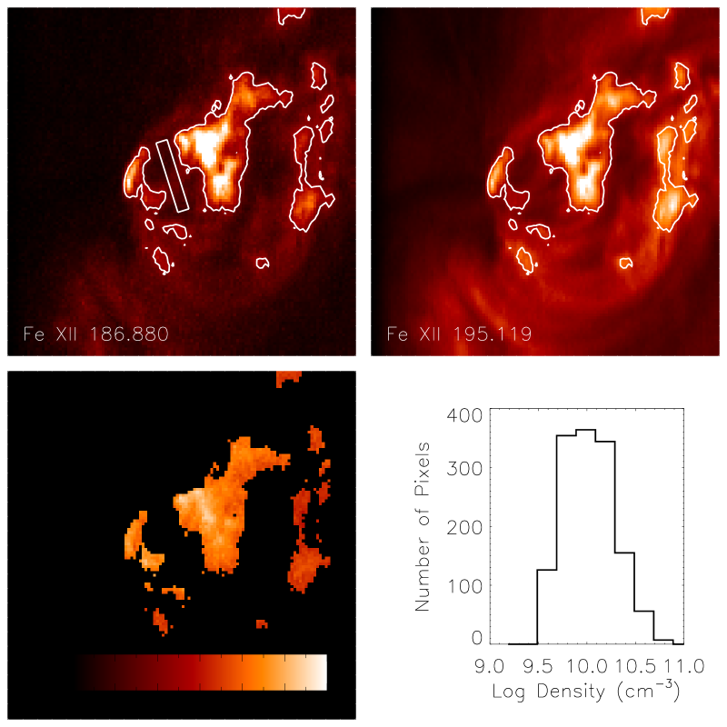
Figure 4: (Upper Panels:) EIS Fe XII 186.880 and 195.119 Å intensities. The regions we define as moss are shown with a contour. (Lower Left Panel:) The density calculated from the line intensity ratio. (Lower Right Panel:) A histogram of the densities.

The top two panels of Figure 4 show the two Fe XII spectral lines. First we use the intensity in the density sensitive line, in this case Fe XII 186.880 Å, to define the moss. We choose a threshold of 1200 ergs cm^-2 s^-1 sr^-1. The moss regions are shown with contours in Figure 4.

Before we calculate the density, we first need to subtract the background emission from the moss regions. Because moss forms the footpoints of the high temperature loops, we are not only looking through the ambient corona, but also through the hot loops above the moss. To account for this, we choose to use the central region of the core (shown as a rectangle in Figure 2) as the background. These background intensities are the same as the apex intensities and given in Table 2.

Using the ratio of the background subtracted intensity and the density sensitive emission measure ratio calculated from CHIANTI 6.0.1, we calculate a density for each moss pixel. The lower left panel shows a density map of the moss regions. The density does not appear to depend on spatial location in the primary moss regions, though the satellite regions to the right typically have lower densities. The lower right panel is a histogram of the number of pixels in the moss region with a given density. The average density is Log n = 10.15 cm^-3 and the standard deviation is 0.49. The largest densities measured in this region are $\sim 5\times 10^{10}$ cm^-3.

3.3 Loop Length

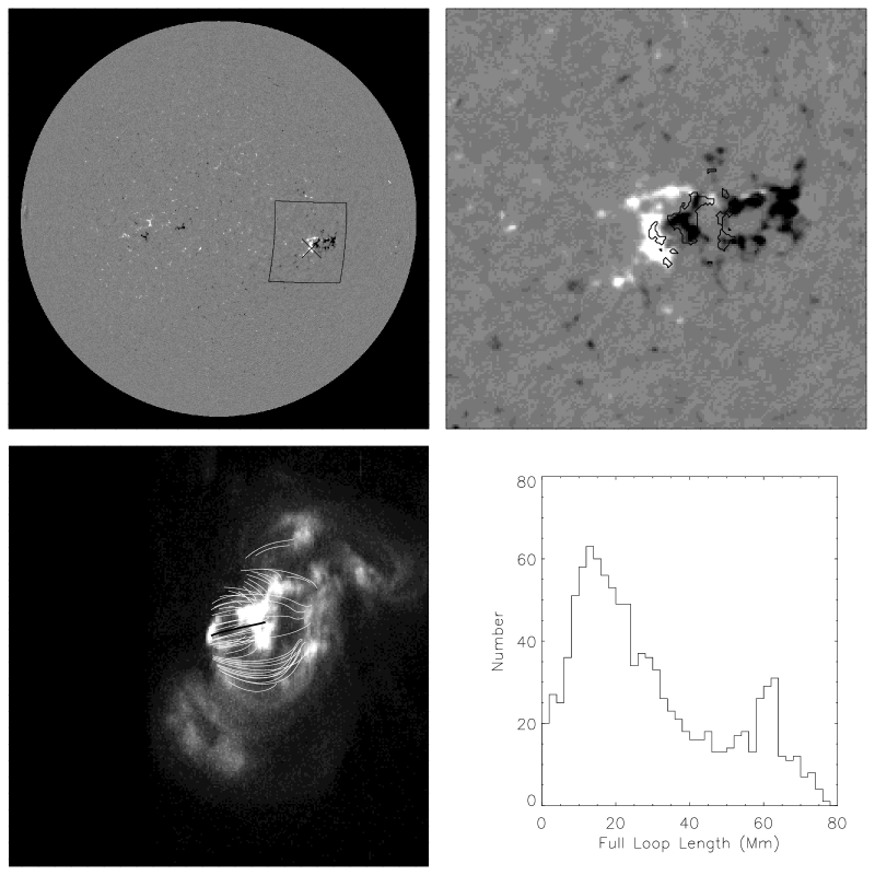
Figure 5: (Upper Left Panel) Full disk magnetic field observations. (Upper Right Panel) Magnetic field around the active region. The contours are the Fe XII 186.880 moss contours. (Lower Left Panel) Field lines from potential field extrapolation. (Lower Right Panel) Histogram of loop lengths of the moss loops.

We approximate the loop lengths and geometries in the active region core using a potential field extrapolation of the photospheric field. First, we start with the full Sun, time-averaged photospheric magnetic field measurements, shown in the upper left panel of Figure 5. We extract a region of full disk magnetic field around the active region, shown with an “X” on the figure. The extracted region, shown in the upper right panel of Figure 5, has been generated so that the pixels are approximately square with the pixel sizes measured in Mm from the center of the active region. Hence, we create a magnetic field coordinate system that is Cartesian around the middle of the active region. We transform the coordinates from the magnetic field coordinate system to the image coordinate system using the transformation matrixes in Aschwanden et al. (1999).

After correcting the magnetic field, we numerically solve the equations $\nabla\times B=0$ and $\nabla\cdot B=0$ to determine the magnetic field vectors in the volume above the photospheric field (e.g., Gary 1989). To define the footpoints of the core loops, we transform the moss footpoints, originally in the image coordinate system, to the magnetic field coordinate system. Recall that the original moss region was co-aligned with the original magnetic field before the region of interest was extracted. Contours of the moss region in the magnetic field coordinate system are shown on the magnetic field image in the top right of Figure 5. We then trace field lines from the moss regions. The x,y coordinates of the moss are defined by the Fe XII 186.880 Å intensity. We assume the height of the moss, and the originating z position of the field line, is 2.5 Mm above the photospheric field. Figure 5 shows a subset of the field lines projected onto the Fe XII 186.880 Å image (lower left panel), as well as a histogram of the full loop lengths of all the field lines in Mm (lower right panel). We find the longest loops associated with this moss region are $<100$ Mm.

4 The Steady Heating Model

In this section, we test whether a simple, steady heating model of this active region core can reproduce both the density-sensitive spectral line intensities in the moss regions and the DEM of the apex emission from the core loops. We predicate this model on four key assumptions derived from the results of previous successful active region models. 1) We assume the geometry of the active region core is well represented by field lines from the potential field extrapolation. 2) We assume the atomic physics of the plasma is well represented by the CHIANTI 6.0.1 package with the ionization balance described by Mazzotta et al. (1998) and abundances described by Feldman et al. (1992). 3) We assume the heating along the loop is well approximated by uniform, steady heating. 4) We assume the cross-sectional area of the loop increases as the magnetic field along the loop decrease, i.e., $A(s)\sim 1/B(s).$

Below we describe the process of finding the best solution for a single field line. We complete this process for each field line, then derive a DEM from the portion of all the field lines that projects into the region of interest shown in Figure 2. To avoid duplicate field lines, we consider field lines traced from only the positive polarity magnetic field.

The example field line is shown as a thick black line in the lower left panel of Figure 5. The field line is 36.7 Mm long. The (x,z) and (y,z) projections of the field line are shown in Figure 6. These figures demonstrate that the field line starts and terminates 2.5 Mm above the solar surface and is roughly semi-circular in the x-projection. The y-projection shows that the field line is slightly inclined. We associate the field line with the background subtracted Fe XII 186.880 and 195.119 Å intensities at its originating footpoint, for this field line, 819.5 and 1213.2 ergs cm^-2 s^-1 sr^-1, respectively.

The first step in formulating the model is guessing the uniform heating rate that will match the Fe XII intensities at the base. Recall that Rosner et al. (1978) determined scaling laws that related the volumetric heating rate to the loop half length in cm and base pressure in dyn cm^-2, i.e.,

$$E=1\times 10^{5}p_{0}^{7/6}/L^{5/6}.$$ (7)

Using the Fe XII line ratio, we calculate a density of $1.0\times 10^{10}$ cm^-3. This density is determined assuming the line intensity is generated by plasma at the temperature of peak formation for Fe XII, Log T = 6.1. We can estimate the base pressure, then, by $p_{0}=2n_{0}kT$ where $k$ is Boltzmann’s constant. For this density, we estimate a base pressure of 3.6 dyn cm^-2. Using this base pressure and the loop half-length in cm, we estimate a uniform heating rate of $9.2\times 10^{-2}$ ergs cm^-3 s^-1.

This value is just an initial estimate of the steady uniform heating rate based on assumptions, such as constant loop pressure and a simplified radiative loss function. Using this estimate, we solve the one-dimensional hydrodynamic equations of continuity, momentum, and energy with a steady-state solver (Schrijver & van Ballegooijen, 2005). The radiative loss function we use to solve the equations was described by Brooks & Warren (2006). The density and temperature along the loop for this heating rate is shown in the bottom two panels in Figure 6 as solid lines .

To calculate the expected intensities in the Fe XII lines from this solution, we integrate the emission measure times the emissivity functions ($\epsilon_{\lambda}$) of Fe XII 186.880 and 195.119 Å, i.e.,

$$I_{\lambda}=\frac{A}{4\pi}\int_{0}^{s_{1}}\epsilon_{\lambda}(T,n)n^{2}ds.$$ (8)

In the above equation, $A$ is the area of a pixel (in this case, 1″) and the upper limit of the integration, $s_{1}$, is the largest distance along the loop that still projects into the original footpoint pixel. In the example, the initial guess of the heating rate of $9.2\times 10^{-2}$ ergs cm^-3 s^-1 produced a Fe XII 186.880 Å intensity of 4910 ergs cm^-2 s^-1 sr^-1 and a Fe XII 195.119 intensity of 6950 ergs cm^-2 s^-1 sr^-1.

The intensity found in Equation 8 would be the intensity if the plasma filled the area of the pixel. To determine the actual percentage of the pixel that contains plasma, or the filling factor, we take the ratio of the observed to modeled Fe XII 195.119 Å intensities. For this simulation, the filling factor is 0.178. Then we multiply the simulated Fe XII 186.880 Å intensity by this filling factor. The Fe XII 186 Å intensity becomes 873 ergs cm^-2 s^-1 sr^-1 which is slightly larger than the observed 819.5 ergs cm^-2 s^-1 sr^-1.

Because the simulated intensity in Fe XII 186.880 Å is too large, we reduce the heating rate by a factor of 2; if it had been too small, we would have increased the heating rate by a factor of 2. Using the new heating rate, we solve again the one-dimensional hydrodynamic equations. The temperature and density solution for a heating rate of $4.6\times 10^{-2}$ ergs cm^-3 s^-1 is shown in the lower panels of Figure 6 with dashed lines. This solution produced a Fe XII 186.880 Å intensity of 755 ergs cm^-2 s^-1 sr^-1.

We now have two different heating rates and two different Fe XII 186.880 Å intensities that bracket the desired Fe XII 186.880 Å intensity. We interpolate between them and predict a heating rate of $6.8\times 10^{-2}$ ergs cm^-3 s^-1 will achieve the desired Fe XII 186.880 Å intensity. The temperature and density solution for this heating rate is shown in Figure 6 with dash-dot lines. The Fe XII 186.880 and 195.119 Å intensities determined from Equation 8 were 1791 and 2702 ergs cm^-2 s^-1 sr^-1, respectively. Using the Fe XII 195.119 Å ratio, we determine a filling factor of 0.457. The simulated Fe XII 186.880 Å intensity is then 819 ergs cm^-2 s^-1 sr^-1 which matched the observed intensity.

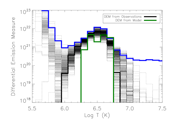
Figure 7: DEM calculated from XRT and EIS data (black). DEM calculated from a steady heating model (green).

We complete this process for all field lines in our study. For 10% of the field lines, the necessary filling factor was $>$ 1; we eliminated these field lines from the study. After the best solution was found for all the field lines, a DEM of was generated from the portion of the density and temperature that projected into the region of interest (the white rectangle shown in Figure 2.) Figure 7 shows the comparison of the DEM calculated from the data (black) and the DEM predicted by the steady heating model (green). The model DEM well approximates the observed DEM around its peak, but the model DEM does not well describe the observations at lower or higher temperatures. We discuss this discrepancy in the next section.

Through this process, we solved for the density and temperature along the loop, as well as the required filling factor to bring the Fe XII intensities into agreement with observations. Figure 8 shows the resulting relationship between the filling factor and temperature (left panel) and loop length and temperature (right panel).

5 Discussion

In this paper, we have combined Hinode EIS and XRT observations to calculate a differential emission measure in an active region core over the neutral line. We also measured the densities at the footpoints of the core loops using the EIS Fe XII line ratio. Using potential field extrapolations of the region we approximate the lengths and geometries of the core loops. Using the density sensitive EIS lines and the loop lengths and geometries, we construct a simple steady heating model. The heating is uniformly deposited along the loop and the cross section of the loop is assumed to expand as magnetic field decreases. Using a code that solves the one-dimensional hydrodynamic equations for steady heating, we adjust the magnitude of the heating rate iteratively until the simulated intensities in the Fe XII 186.880 and 195.119 spectral lines match the observed intensities to within 1%. We then construct a DEM from the solutions and compare with the observed DEM.

In the temperature range 6.3 $<$ Log T $<$ 6.7, the model DEM is in general agreement with the observations. The magnitude of the model DEM is approximately the same as the magnitude of the observed DEM. The median temperature of the model DEM (Log $T=6.5$ MK) is the same as the temperature of the peak of the observed DEM. This good agreement was arrived at using relatively few assumptions: potential field geometry, CHIANTI atomic physics, uniform, steady heating, and loop area inversely proportional to the magnetic field. These assumptions were motivated by successful parameter space searches in previous studies.

Unlike previous studies, however, no additional “fudge factors” were used, such as a filling factor, to force agreement between the observations and the model. Because this study relies on density sensitive line intensities, the areal filling factor is determined through the model calculation. After making these four key assumptions, there are no additional assumptions that could be made that could, for instance, artificially raise or lower the temperatures in the loops. In fact, the maximum and minimum temperature of model DEM are defined by the maximum and minimum density and loop length shown in Figures 4 and 5. We determined the maximum electron density in the moss was $\sim 5\times 10^{10}$ cm^-3 and the maximum loop length measured from potential field extrapolations was $\sim 100$ Mm. The moss densities were measured with density sensitive Fe xii lines formed at $1.5$ MK. For the resulting pressure ($\sim 20$ dyn cm²) and half-length, we estimate the maximum apex temperature of loops for high-frequency heating is 6.5 MK from the RTV scaling law which is in agreement with the maximum temperature of the model DEM. Observations of significant emission at higher temperatures would have indicated a disagreement with the steady heating model.

At temperatures much lower or higher than the peak temperature (Log T $<$ 6.1 or Log T $>$ 6.7), the observed DEM is not well constrained and comparisons with the model are not meaningful. At mid-range, “warm” temperatures (6.1 $<$ Log T $<$ 6.3), however, the observed DEM is well constrained and significantly larger than the DEM from the model. There are (at least) two possible explanations for this discrepancy. 1) The warm emission is from the overlying arcade of warm loops that was not removed in the original background subtraction. Figure 1 supports this view. The Fe XII raster shows the presence of many overlying loops that are not confined to the core loops bright in the XRT C_poly image. 2) The warm emission is truly from the core loops, casting serious doubt on the steady heating model. Another heating model, such as the infrequent heating or “nanoflare’ model (Cargill & Klimchuk, 1997) must be operating.

The series of TRACE 171 Å images taken throughout the time period under investigation seem to support option (1). The 171 Å filter has a peak response of Log T $\approx$ 6.0, and is extremely sensitive to these warm loops. The TRACE images show a series of these loops, with a detailed geometry that would remain even after our careful attempts at background subtraction. Based on these comparisons, we conclude that the steady heating model agrees with the observed properties in the active region core, including the density sensitive line ratios in the footpoints of core loops, the distribution of high temperature emission at the apex of the core loops, and the appearance of warm loops in the series of TRACE images. Regardless, additional modeling efforts are underway to test whether the low-frequency nanoflare model (as described by Cargill & Klimchuk 1997, 2004; Klimchuk et al. 2008; Klimchuk 2009) could be operating in active region cores. Initial studies characterizing the DEM predicted by long nanoflare storms are underway (Klimchuk et al., 2008; Susino et al., 2010; Tripathi et al., 2011; Warren et al., 2011; Mulu-Moore et al., 2011).

In this paper, we chose to use the cooler Fe XII 186.880/195.119 Å line ratio in the moss region and the hotter Fe XIII 202.044/203.826 Å line ratio to determine the density in the core region. It has been well documented, however, that densities calculated from the Fe XII line ratio could be as much as a factor of 2 more than the densities calculated from other EIS line ratios (Warren et al., 2010). For steady heating, the apex temperature of a loop is proportional to the cube root of the base pressure, i.e., $T_{\rm apex}\sim(p_{0})^{1/3}$, so if the density were a factor of 2 lower, the temperatures in the loops would be a factor of 1.25 lower which would shift the model DEM to lower temperatures. Currently, the average median temperature of the simulated loops is 3.1 MK. If the true densities were a factor of 2 lower, it would shift this average temperature to 2.5 MK.

The densities measured in this analysis are in good agreement with other measurements of moss densities (Tripathi et al., 2008, 2010). The emission measure curve found in this analysis, however, is significantly steeper in the temperature range of 6.0 $<$ Log T $<$ 6.5 than have been found in previous emission measure calculations. We find the emission measure curve in this temperature range can be approximated as a power-law, i.e., $EM\sim T^{b}$, with an index, $b$, of 3.2, while previous results have found $1<b<3$ (e.g., Dere & Mason, 1993; Brosius et al., 1996). These previous results averaged the intensities over large fields of view which included both high temperature loops, moss, and extended EUV loops. Two recent analyses of the emission measure distribution of inter-moss regions determined a range of indices $2.1<b<3.4$ (Warren et al., 2011; Tripathi et al., 2011). It is clear a systematic study of the emission measure distributions of inter-moss regions is required to fully characterize the temperature structure of the active region core.

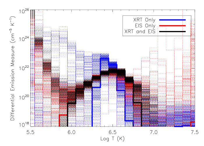
Figure 9: DEM calculated from XRT intensities only (blue), from EIS intensities only (red) and from the combined XRT and EIS data set (black).

In this paper, we combine XRT and EIS data sets to calculate a differential emission measure, similar to Schmelz et al. (2010). Figure 9 demonstrates the power of this combined data set compared to using the data sets individually. The DEM shown in blue is calculated from the XRT intensities alone, the DEM shown in red is calculated from the EIS line intensities alone, and the DEM shown in black is the combined data set. Comparing the combined DEM with the individual instrument DEMs, we see the combined DEM agrees well with the EIS DEM in the range 6.0 $<$ Log T $<$ 6.5, however the EIS DEM greatly overestimates the true DEM at high temperatures. The DEM calculated from the XRT data is significantly different from the combined DEM at all temperatures. The peak of the XRT only DEM is larger and at a lower temperature than the peak of the combined DEM. Because the EIS data highly constrains the combined DEM at Log T = 6.5, it forces the emission in the X-ray filters to high temperatures, causing the combined DEM to be broader than the XRT only DEM.

We have not considered any cross-calibration factor for these two instruments in this analysis. Testa et al. (2011) completed an extensive cross-calibration effort and determined a cross-calibration factor of $\sim 2$ may be necessary. To determine the calibration factor, they used EIS lines with significant temperature overlap of the XRT filters. The data set presented in this analysis, however, contained only the Fe XVII 254.870 Å line that overlaps the XRT temperature range. Furthermore, additional studies of combined data sets that did have significant temperature overlap (Warren et al., 2011; O’Dwyer et al., 2011) did not find the need to include a cross-calibration factor. Because the XRT contamination varies in time, it is difficult to assess the relative calibration of the two instruments.

Finally, our DEM curve for AR 10955, which used XRT data from 16:00 UT (see Table 1), shows no significant hot plasma with Log T $\gtrsim$ 7.0; the blue line in Figure 3 shows our limited sensitivity to such plasma, given the observed count rates and errors in the count rates. This active region, however, has been studied previously. Schmelz et al. (2009b) used a similar XRT data set from 18:00 UT (approximately two hours after the XRT data considered in this paper) to determine the DEM for a portion of the active region to the north-west of the core. Schmelz et al. (2009a) used the 18:00 UT XRT data as well as RHESSI upper limits to modify and further constrain the DEM. Both papers found that considerable emission in the high temperature range was required to account for the small but significant signal detected in the XRT Be_thick filter.

Although both the 16:18 UT and 18:00 UT Be_thick images had the same resolution, field-of-view, and exposure time, the earlier image analyzed in this paper does not show a significant signal, where the later one analyzed by Schmelz et al. (2009b, a) does. The GOES signal for 2007 May 13 was low all day, rarely getting above level A0. There were two small A4 flares from AR 10955 at 11:20 and 11:35 UT, before both sets of XRT observations, but then the region settled down to its sub-A0 level again. It maintained the quiescent stage through our 16:00 UT observations, only to rise again to A1-A2 from 17:00 UT to just past 18:00 UT when there was another small A7 flare. One possible explanation for the different DEM results is that AR 10955 appears to have been in a more quiescent state during our 16:00 UT observations, and in a somewhat heightened state of activity (right before the small A7 flare) during their 18:00 UT observations. It would be interesting to repeat the XRT-RHESSI DEM analysis for a stronger, more powerful active region with a significant signal in the XRT Be_thick filter to see if the high-temperature plasma is detectable.

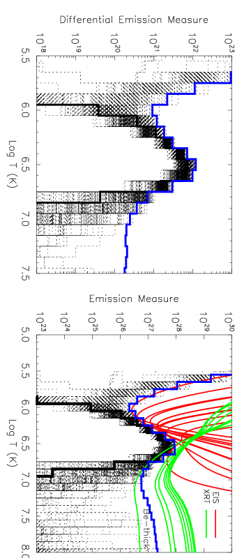
Figure 3: (Left Panel:) The thick solid lines show the best DEM for the input XRT and EIS intensities and the dotted lines surrounding the solid line gives an estimate of the error in the DEM. The blue line represents the maximum emission that can be added to a single temperature bin without changing the modeled intensity by more than the observed errors. (Right Panel:) The integral form of the DEM and corresponding EM loci curves. The EIS EM loci curves are shown in pink and the XRT EM loci curves are shown in green.

Figure 6: (Upper Panels:) The field line projected in (x,z) and (y,z). (Lower Left Panel:) The temperature as a function of position along the loop for three different heating rates. (Lower Right Panel:) The density as a function of position along the loop for three different heating rates.

Figure 8: (Left Panel:) Filling factor as a function of maximum temperature in the loop. (Right Panel:) Maximum temperature in a loop as a function of the full loop length.

Table 1: XRT Data from 2007 May 13

Filter	Time (UT)	Exposure (long)	Time (UT)	Exposure (short)
Al_mesh	16:21:05	4.10 sec	16:20:11	0.18 sec
C_poly	16:26:20	8.20 sec	16:25:22	0.51 sec
Ti_poly	16:19:52	8.20 sec	16:19:42	0.51 sec
Al_poly-Ti_poly	16:22:55	16.4 sec	16:21:50	1.45 sec
C_poly-Ti_poly	16:24:38	16.4 sec	16:23:37	1.03 sec
Be_thin	16:28:49	23.1 sec	16:28:13	1.03 sec
Be_med	16:30:23	46.3 sec	16:29:32	2.05 sec
Al_thick	16:18:44	46.3 sec	16:18:18	16.4 sec
Be_thick	16:17:02	65.5 sec	——	—–

Table 2: EIS and XRT Intensities

Line/Filter	I	$\sigma$	IDEM	I/IDEM
Fe X 177.239	254	194	239	1.1
Fe XI 180.401	482	218	637	0.76
Fe XII 186.880	587	149	434	1.4
Fe XII 195.119	768	259	941	0.81
Fe XIII 203.826	1725	414	1153	1.5
Fe XIII 202.044	601	213	421	1.4
Fe XIV 264.787	1016	241	1189	0.85
Fe XIV 274.203	870	215	864	1.0
Fe XV 284.160	9450	2150	11570	0.82
Fe XVI 262.984	1140	257	852	1.3
Fe XVII 254.870	33	16	58	0.57
Al_mesh	1940	390	1406	1.4
C_poly	1226	247	1075	1.1
Ti_poly	876	177	690	1.3
Al_poly/Ti_poly	601	121	475	1.3
C_poly/Ti_poly	435	88	385	1.1
Be_thin	351	71	326	1.1
Be_med	67.3	14.0	71	0.95
Al_thick	2.43	0.82	3.23	0.75
Be_thick	0.041	0.058	0.12	0.32

References

- Antiochos et al. (2003) Antiochos, S. K., Karpen, J. T., DeLuca, E. E., Golub, L., & Hamilton, P. 2003, ApJ, 590, 547
- Aschwanden et al. (1999) Aschwanden, M. J., Newmark, J. S., Delaboudinière, J., Neupert, W. M., Klimchuk, J. A., Gary, G. A., Portier-Fozzani, F., & Zucker, A. 1999, ApJ, 515, 842
- Brooks & Warren (2006) Brooks, D. H., & Warren, H. P. 2006, ApJS, 164, 202
- Brooks & Warren (2009) Brooks, D. H., & Warren, H. P. 2009, ApJ, 703, L10
- Brosius et al. (1996) Brosius, J. W., Davila, J. M., Thomas, R. J., & Monsignori-Fossi, B. C. 1996, ApJS, 106, 143
- Brown et al. (2007) Brown, C. M., et al. 2007, PASJ, 59, 865
- Cargill & Klimchuk (1997) Cargill, P. J., & Klimchuk, J. A. 1997, ApJ, 478, 799
- Cargill & Klimchuk (2004) Cargill, P. J., & Klimchuk, J. A. 2004, ApJ, 605, 911
- Culhane et al. (2007) Culhane, J. L., et al. 2007, Sol. Phys., 243, 19
- Dere & Mason (1993) Dere, K. P., & Mason, H. E. 1993, Sol. Phys., 144, 217
- Feldman et al. (1992) Feldman, U., Mandelbaum, P., Seely, J. F., Doschek, G. A., & Gursky, H. 1992, ApJS, 81, 387
- Gary (1989) Gary, G. A. 1989, ApJS, 69, 323
- Golub et al. (2007) Golub, L., et al. 2007, Sol. Phys., 243, 63
- Golub et al. (2004) Golub, L., Deluca, E. E., Sette, A., & Weber, M. 2004, in Astronomical Society of the Pacific Conference Series, Vol. 325, The Solar-B Mission and the Forefront of Solar Physics, ed. T. Sakurai & T. Sekii, 217
- Jordan et al. (1987) Jordan, C., Ayres, T. R., Brown, A., Linsky, J. L., & Simon, T. 1987, MNRAS, 225, 903
- Klimchuk (2000) Klimchuk, J. A. 2000, Sol. Phys., 193, 53
- Klimchuk (2006) Klimchuk, J. A. 2006, Sol. Phys., 234, 41
- Klimchuk (2009) Klimchuk, J. A. 2009, in Astronomical Society of the Pacific Conference Series, Vol. 415, Astronomical Society of the Pacific Conference Series, ed. B. Lites, M. Cheung, T. Magara, J. Mariska, & K. Reeves, 221
- Klimchuk et al. (2008) Klimchuk, J. A., Patsourakos, S., & Cargill, P. J. 2008, ApJ, 682, 1351
- Korendyke et al. (2006) Korendyke, C. M., et al. 2006, Appl. Opt., 45, 8674
- Kosugi et al. (2007) Kosugi, T., et al. 2007, Sol. Phys., 243, 3
- Lang et al. (2006) Lang, J., et al. 2006, Appl. Opt., 45, 8689
- Lundquist et al. (2008) Lundquist, L. L., Fisher, G. H., & McTiernan, J. M. 2008, ApJS, 179, 509
- Martens et al. (2000) Martens, P. C. H., Kankelborg, C. C., & Berger, T. E. 2000, ApJ, 537, 471
- Mazzotta et al. (1998) Mazzotta, P., Mazzitelli, G., Colafrancesco, S., & Vittorio, N. 1998, A&AS, 133, 403
- Mulu-Moore et al. (2011) Mulu-Moore, F. M., Winebarger, A. R., & Warren, H. P. 2011, ApJ, accepted
- Mulu-Moore et al. (2011) Mulu-Moore, F. M., Winebarger, A. R., Warren, H. P., & Aschwanden, M. 2011, ApJ, accepted
- Narukage et al. (2011) Narukage, N., et al. 2011, Sol. Phys., 269, 169
- O’Dwyer et al. (2011) O’Dwyer, B., Del Zanna, G., Mason, H. E., Sterling, A. C., Tripathi, D., & Young, P. R. 2011, A&A, 525, A137
- Parker (1972) Parker, E. N. 1972, ApJ, 174, 499
- Reale (2010) Reale, F. 2010, Living Reviews in Solar Physics, 7, 5
- Rosner et al. (1978) Rosner, R., Tucker, W. H., & Vaiana, G. S. 1978, ApJ, 220, 643
- Schmelz et al. (2009a) Schmelz, J. T., et al. 2009a, ApJ, 704, 863
- Schmelz et al. (2009b) Schmelz, J. T., Saar, S. H., DeLuca, E. E., Golub, L., Kashyap, V. L., Weber, M. A., & Klimchuk, J. A. 2009b, ApJ, 693, L131
- Schmelz et al. (2010) Schmelz, J. T., Saar, S. H., Nasraoui, K., Kashyap, V. L., Weber, M. A., DeLuca, E. E., & Golub, L. 2010, ApJ, 723, 1180
- Schrijver et al. (2004) Schrijver, C. J., Sandman, A. W., Aschwanden, M. J., & DeRosa, M. L. 2004, ApJ, 615, 512
- Schrijver & van Ballegooijen (2005) Schrijver, C. J., & van Ballegooijen, A. A. 2005, ApJ, 630, 552
- Serio et al. (1981) Serio, S., Peres, G., Vaiana, G. S., Golub, L., & Rosner, R. 1981, ApJ, 243, 288
- Susino et al. (2010) Susino, R., Lanzafame, A. C., Lanza, A. F., & Spadaro, D. 2010, ApJ,
- Testa et al. (2011) Testa, P., Reale, F., Landi, E., DeLuca, E. E., & Kashyap, V. 2011, ApJ, 728, 30
- Tripathi et al. (2011) Tripathi, D., Klimchuk, J., & Mason, H. 2011, ApJ, submitted
- Tripathi et al. (2010) Tripathi, D., Mason, H. E., Del Zanna, G., & Young, P. R. 2010, A&A, 518, A42
- Tripathi et al. (2008) Tripathi, D., Mason, H. E., Young, P. R., & Del Zanna, G. 2008, A&A, 481, L53
- Tsuneta et al. (1991) Tsuneta, S., et al. 1991, Sol. Phys., 136, 37
- Ugarte-Urra et al. (2009) Ugarte-Urra, I., Warren, H. P., & Brooks, D. H. 2009, ApJ, 695, 642
- Ugarte-Urra et al. (2006) Ugarte-Urra, I., Winebarger, A. R., & Warren, H. P. 2006, ApJ, 643, 1245
- Warren et al. (2011) Warren, H. P., Brooks, D., & Winebarger, A. R. 2011, ApJ, submitted
- Warren et al. ( 2008) Warren, H. P., Feldman, U. & Brown, C. M. 2008, ApJ, 685, 1277
- Warren & Winebarger (2006) Warren, H. P., & Winebarger, A. R. 2006, ApJ, 645, 711
- Warren & Winebarger (2007) Warren, H. P., & Winebarger, A. R. 2007, ApJ, 666, 1245
- Warren et al. (2010) Warren, H. P., Winebarger, A. R., & Brooks, D. H. 2010, ApJ, 711, 228
- Warren et al. (2002) Warren, H. P., Winebarger, A. R., & Hamilton, P. S. 2002, ApJ, 579, L41
- Warren et al. (2003) Warren, H. P., Winebarger, A. R., & Mariska, J. T. 2003, ApJ, 593, 1174
- Weber et al. (2004) Weber, M. A., Deluca, E. E., Golub, L., & Sette, A. L. 2004, in IAU Symposium, Vol. 223, Multi-Wavelength Investigations of Solar Activity, ed. A. V. Stepanov, E. E. Benevolenskaya, & A. G. Kosovichev, 321
- Winebarger & Warren (2005) Winebarger, A. R., & Warren, H. P. 2005, ApJ, 626, 543
- Winebarger et al. (2008) Winebarger, A. R., Warren, H. P., & Falconer, D. A. 2008, ApJ, 676, 672
- Winebarger et al. (2003) Winebarger, A. R., Warren, H. P., & Seaton, D. B. 2003, ApJ, 593, 1164