Periodic Anderson model with correlated conduction electrons:
variational and exact diagonalization study

Abstract

We investigate an extended version of the periodic Anderson model (the so-called periodic Anderson-Hubbard model) with the aim to understand the role of interaction between conduction electrons in the formation of the heavy-fermion and mixed-valence states. Two methods are used: (i) variational calculation with the Gutzwiller wave function optimizing numerically the ground-state energy and (ii) exact diagonalization of the Hamiltonian for short chains. The $f$-level occupancy and the renormalization factor of the quasiparticles are calculated as a function of the energy of the $f$-orbital for a wide range of the interaction parameters. The results obtained by the two methods are in reasonably good agreement for the periodic Anderson model. The agreement is maintained even when the interaction between band electrons, $U_{d}$, is taken into account, except for the half-filled case. This discrepancy can be explained by the difference between the physics of the one- and higher dimensional models. We find that this interaction shifts and widens the energy range of the bare $f$-level, where heavy-fermion behavior can be observed. For large enough $U_{d}$ this range may lie even above the bare conduction band. The Gutzwiller method indicates a robust transition from Kondo insulator to Mott insulator in the half-filled model, while $U_{d}$ enhances the quasi-particle mass when the filling is close to half filling.

I Introduction

Rare-earth materials exhibit numerous remarkable phenomena such as heavy-fermion behavior, valence fluctuations, and unconventional superconductivity. The simplest model that can account for these phenomena is the periodic Anderson model (PAM), where mobile conduction electrons in a broad band of width $W$ can hybridize with immobile $f$-electrons sitting at the lattice sites. The Coulomb repulsion is taken into account between the $f$-electrons only. Written in a mixed, Bloch and Wannier representation, this model is defined by the Hamiltonian

$$\begin{split}\mathcal{H}=&\sum_{\boldsymbol{k},\sigma}\varepsilon_{d}(\boldsymbol{k})\hat{d}_{\boldsymbol{k}\sigma}^{\dagger}\hat{d}^{\phantom{\dagger}}_{\boldsymbol{k}\sigma}+\varepsilon_{f}\sum_{j,\sigma}\hat{n}^{f}_{j\sigma}\\ &-V\sum_{j,\sigma}(\hat{f}_{j\sigma}^{\dagger}\hat{d}^{\phantom{\dagger}}_{j\sigma}+\hat{d}_{j\sigma}^{\dagger}\hat{f}^{\phantom{\dagger}}_{j\sigma})+U_{f}\sum_{j}\hat{n}^{f}_{j\uparrow}\hat{n}^{f}_{j\downarrow},\end{split}$$ (1)

where $\hat{d}_{\boldsymbol{k}\sigma}^{\dagger}$ ($\hat{d}_{\boldsymbol{k}\sigma}^{\phantom{\dagger}}$) is the creation (annihilation) operator of conduction electrons with wave vector $\boldsymbol{k}$ and spin $\sigma$, while $\hat{f}_{j\sigma}^{\dagger}$ ($\hat{f}_{j\sigma}^{\phantom{\dagger}}$) denotes the creation (annihilation) operator of $f$-electrons at site $\boldsymbol{r}_{j}$ in an arbitrary dimensional lattice with $N$ lattice sites, $\hat{n}^{f}_{j\sigma}=\hat{f}_{j\sigma}^{\dagger}\hat{f}_{j\sigma}^{\phantom{\dagger}}$ is the number operator of $f$-electrons at site $\boldsymbol{r}_{j}$, and $\hat{n}^{d}_{j\sigma}$ is defined similarly. The hybridization matrix element between $f$- and $d$-states is denoted by $V$, and $U_{f}$ is the strength of the on-site Coulomb repulsion between $f$-electrons. We consider the nondegenerate case, i.e., one $d$- and one $f$-orbital per site is assumed. Therefore, owing to the two possible orientations of the spin, the average number of $d$- and $f$-electrons per site, $n_{d}$ and $n_{f}$, respectively, can vary between zero and two. The filling will refer to the ratio of the total electron density per site ($n_{d}+n_{f}$) and the maximally allowed electron density ($n_{\rm max}=4$).

Although it has been investigated for several decades,Review this model and its extended versions are still in the forefront of condensed-matter physics. Since exact results are available only for certain special cases,Exact besides the large number of perturbative studies nonperturbative techniques have also been developed to go beyond the weak-coupling limit. The Gutzwiller variational methodGutzwiller:original has been applied by several authors.Rice&Ueda:variational ; Brandow:1986 ; Varma:1986 ; Shiba:1986 ; Oguchi:1987 ; Fazekas:variational ; Lamba:variational In this method, an uncontrolled approximation (the so-called Gutzwiller approximationGutzwiller:original ) is often used to calculate expectation values with the correlated wave function. Metzner and VollhardtVollhardt:cikk87 have shown that the expectation values can be evaluated exactly in one dimension. Later they considered the limit of large dimensions,Vollhardt:cikk89 where analytic treatment is possible. GebhardGebhard:cikk developed a technique to calculate expectation values in a controlled expansion in the inverse of the degeneracy of the $f$-level and in the inverse of the dimension of the lattice. He showed that the Gutzwiller approximation provides exact results in the limit of large dimensions. Moreover, in this limit this method is equivalent to the slave-boson mean-field theory of Kotliar and Ruckenstein.Kotliar:cikk ; Moller:cikk Later on, the dynamical mean-field theory,DMFT:review which, too, is exact in the limit of infinite dimensions, has been applied to the periodic Anderson model by several authorsOhkawa ; Jarrell1 ; Jarrell2 ; Saso to better understand the main features of the model. To avoid the problem related to the Gutzwiller approximation, ShibaShiba:1986 applied the variational Monte Carlo method. The PAM was investigated also by using the projector-based renormalization methodHubsch:cikk for arbitrary degeneracy of the $f$-level. The ferromagnetic properties of the PAM have been studied with the density-matrix renormalization group.Guerrero:DMRG

In view of the widespread application of the Gutzwiller approximation, it is important to know how reliable this method is. As will be demonstrated in this paper by comparing the results with those of exact diagonalization, the Gutzwiller method gives – in spite of its limitations – reliable results for the number of electrons occupying the $f$-orbital. The $f$-level occupancy is a significant quantity, for it has recently been proposedMiyake_cikk and experimentally verifiedRueffPRL_meres:cikk that the pressure induced enhancement of the superconducting transition temperature of Ce based compounds, CeCu₂(Ge,Si)₂ is closely related to a sharp change of the valence of Ce.

Several extensions of the periodic Anderson model have been considered so far in order to make the model more realistic. It was found that nearest-neighbor interaction between $f$-electrons affects the stability of the magnetic ground state in the Kondo regime.Lamba:NN_int On the other hand, the on-site interaction between $d$- and $f$-electrons ($U_{df}\sum_{\boldsymbol{j},\sigma,\sigma^{\prime}}\hat{n}^{f}_{j\sigma}\hat{n}^{d}_{j\sigma^{\prime}}$) influences drastically the occupation number of $f$-electrons.Hirashima:DMFT_Udf It has been shown that a large $U_{df}$ destroys the Kondo state and narrows the intermediate valence regime.Miyake_cikk ; Hirashima:DMFT_Udf Its treatment in the framework of the Gutzwiller method is, however, quite cumbersome. In our previous work Hagymasi&Itai&Solyom:cikk we assumed a special form for this interaction, $\widetilde{U}_{df}\sum_{\boldsymbol{j}}\hat{n}^{f}_{j\uparrow}\hat{n}^{f}_{j\downarrow}\hat{n}^{d}_{j\uparrow}\hat{n}^{d}_{j\downarrow}$, and pointed out that the intermediate-valence regime is narrowed in the presence of this interaction.

The model we study in the second part of this paper includes the interaction between conduction electrons ($d$-electrons). Although the corresponding impurity problem has been examined thoroughly in several papers,Furusaki:cikk ; Li:cikk ; Frojd:cikk ; Schork:cikk ; Khaliullin:cikk ; Igarashi:cikk ; Igarashi:cikk1 ; Schork:cikk1 only a few results are available on the lattice problem.Itai:variational ; Koga:DMFT_Ud ; Schork:DMFT_Ud ; Kawakami:Ud Fulde and coworkersFulde93 have pointed out that the heavy-fermion propertiesBrugger:exp of Ce-doped Nd₂CuO₄ cannot be explained without taking correlations between conduction electrons into account. Although it has been shownItai:variational that correlations between conduction electrons may increase the effective mass, and the competition between Coulomb repulsion in the $d$- and $f$-electron subsystem may lead to a transition from Kondo to Mott insulator, the role of the electron-electron interaction in the conduction electron subsystem is not fully clarified. In this paper we calculate the number of $f$-electrons per site and the probability of double occupancy of $f$-orbitals as a function of the energy of the bare $f$-level, the hybridization, and the $f$-$f$ and $d$-$d$ Coulomb interactions. The calculations are carried out for a wide range of parameters of the model Hamiltonian, and the regions for Kondo-like behavior as well as for valence fluctuations are determined.

The paper is divided into two main parts. Firstly, we investigate the reliability of the Gutzwiller method. We compare the variational results with those of exact diagonalization on finite chains. Secondly, we analyze what happens when the interaction between conduction electrons, $U_{d}$, is switched on.

II Variational calculation and exact diagonalization

II.1 Variational calculation

First of all, following Ref. [Itai:variational, ] we summarize briefly the main steps of the variational calculation for the original periodic Anderson model without interaction between conduction electrons, $U_{d}=0$. In this paper we restrict ourselves to the paramagnetic case, i.e., the number of up-spin electrons, $N_{\uparrow}$, equals that of down-spin electrons, $N_{\downarrow}$. Furthermore, we carry out the explicite calculation only for the system being half-filled or less than that, since the results for the system more than half-filled can be obtained straightforwardly owing to the electron-hole symmetry.

The trial wave function is chosen in the form

$$|\Psi\rangle=\hat{P}_{\rm G}^{f}\prod_{\boldsymbol{k}}\prod_{\sigma}\left[u_{\boldsymbol{k}}\hat{f}_{\boldsymbol{k}\sigma}^{\dagger}+v_{\boldsymbol{k}}\hat{d}_{\boldsymbol{k}\sigma}^{\dagger}\right]|0\rangle,$$ (2)

where the mixing amplitudes $u_{\boldsymbol{k}}$ and $v_{\boldsymbol{k}}$ are variational parameters. $\hat{P}_{\rm G}^{f}$ is the Gutzwiller projector for $f$-electrons:

$$\hat{P}_{\rm G}^{f}=\prod_{\boldsymbol{j}}\left[1-(1-\eta_{f})\hat{n}_{j\uparrow}^{f}\hat{n}_{j\downarrow}^{f}\right],$$ (3)

where the variational parameter $\eta_{f}$ is controlled by $U_{f}$. We use the Gutzwiller approximation to evaluate the expectation values. Optimizing with respect to the mixing amplitudes, we obtain

$$\mathcal{E}=\frac{1}{N}\sum_{\boldsymbol{k}\in\mathrm{FS}}\left[\varepsilon_{d}(\boldsymbol{k})+\tilde{\varepsilon}_{f}-\sqrt{\big{[}\varepsilon_{d}(\boldsymbol{k})-\tilde{\varepsilon}_{f}\big{]}^{2}+4\tilde{V}^{2}}\right]$$

$$+(\varepsilon_{f}-\tilde{\varepsilon}_{f})n_{f}+U_{f}\nu_{f}$$ (4)

for the ground-state energy per site, where $n_{f}$ and $\nu_{f}$ denote the number of $f$-electrons per site and the density of doubly occupied $f$-sites, respectively, $\tilde{V}=V\sqrt{q_{f}}$ is the renormalized hybridization amplitude with

$$q_{f} = \frac{1}{\left(1-\frac{n_{f}}{2}\right)\frac{n_{f}}{2}}\Bigg{[}\sqrt{\left(\frac{n_{f}}{2}-\nu_{f}\right)\nu_{f}}$$ (5)

$$\phantom{+++}+\sqrt{\left(\frac{n_{f}}{2}-\nu_{f}\right)(1-n_{f}+\nu_{f})}\Bigg{]}^{2},$$

while the renormalized energy of the $f$-level, $\tilde{\varepsilon}_{f}$ has to be determined self-consistently from the condition

$$n_{f}=\frac{1}{N}\sum_{\boldsymbol{k}\in\mathrm{FS}}\left[1+\frac{\varepsilon_{d}(\boldsymbol{k})-\tilde{\varepsilon}_{f}}{\sqrt{\big{[}\varepsilon_{d}(\boldsymbol{k})-\tilde{\varepsilon}_{f}\big{]}^{2}+4{\tilde{V}}^{2}}}\right].$$ (6)

The $\boldsymbol{k}$ sum in Eqs. (4) and (6) [and later on, Eqs. (19) and (21) in the next section] extends over the $U_{f}=U_{d}=0$ Fermi sea in a manner familiar from the periodic Anderson model,Fazekas:variational since the Gutzwiller method respects Luttinger’s theorem and leaves the Fermi volume unchanged.

The quantities $n_{f}$ and $\nu_{f}$, and thereby $\tilde{\varepsilon}_{f}$ and $q_{f}$ depend on the as yet undetermined variational parameter $\eta_{f}$. Optimizing with respect to this parameter is equivalent to minimizing the energy with respect to $n_{f}$ and $\nu_{f}$, which leads to

$${\tilde{\varepsilon}}_{f} = \frac{\partial{\cal E}}{\partial q_{f}}\cdot\frac{\partial q_{f}}{\partial n_{f}}+\frac{\partial{\cal E}}{\partial{\tilde{\varepsilon}}_{f}}\cdot\frac{\partial{\tilde{\varepsilon}}_{f}}{\partial n_{f}},$$ (7)

$$-U_{f} = \frac{\partial{\cal E}}{\partial q_{f}}\cdot\frac{\partial q_{f}}{\partial{\nu_{f}}}+\frac{\partial{\cal E}}{\partial{\tilde{\varepsilon}}_{f}}\cdot\frac{\partial{\tilde{\varepsilon}}_{f}}{\partial\nu_{f}}.$$ (8)

These equations have to be solved together with the self-consistency condition (6).

The summation over $\boldsymbol{k}$ in Eqs. (4) and (6) could be carried out numerically for a realistic dispersion curve $\varepsilon_{d}(\boldsymbol{k})$, but the variational procedure, i.e., the numerical optimization of the ground-state energy with the self-consistency condition (6), would be very cumbersome. Instead of that, we assume a constant density of states, $\rho(\varepsilon)=1/W$, in the interval $\varepsilon\in[-W/2,W/2]$, since then the energy density and the self-consistent value of $\tilde{\varepsilon}_{f}$ can be expressed analytically from Eqs. (4) and (6) as a function of $n_{f}$ and $\nu_{f}$.

However, the self-consistent solution of the minimum conditions for $n_{f}$ and $\nu_{f}$ can be found analytically only in special cases, e.g., for $U_{f}\rightarrow\infty$, when $V\ll W$.Itai:variational In this paper we will solve Eqs. (7) and (8) numerically for various values of $V$, $U_{f}$, and $\varepsilon_{f}$ in order to determine the range of parameters for the Kondo or intermediate-valence behavior, and for the crossover regime between them.

Firstly, we calculate the $U_{f}$- and $\varepsilon_{f}$-dependence of the $f$-level occupancy, $n_{f}$, and of the renormalization factor $q_{f}$ in the half-filled case, where the total number of electrons equals the sum of the number of $d$- and $f$-orbitals (the electron density per site $n=n_{d}+n_{f}=2$), and in the 1/3-filled case ($n=4/3$). Other fillings will be discussed later in the next subsection, where we compare the results with those obtained by exact diagonalization.

We note that our model with $n$ electrons can be mapped onto a model with $n$ holes ($4-n$ electrons), provided that the energy level of the $f$-hole is chosen as $-(\varepsilon_{f}+U_{f})$. Therefore, the results for $n>2$ can be obtained straightforwardly from those for $n<2$. Owing to this symmetry in the special, symmetric half-filled case, when $n\!=\!2$ and the bare $f$-level is located at $\varepsilon_{f}=-U_{f}/2$, both $n_{f}$ and $n_{d}$ are exactly equal to 1.

The $f$-level occupancy is displayed as a function of the bare $f$-level energy and of $U_{f}$ for $V/W=0.1$ in the half-filled and 1/3-filled cases, respectively, in Figs. 1 and 2. Five different regimes can be distinguished. When $\varepsilon_{f}+U_{f}$ lies below the conduction band, all electrons occupy $f$-orbitals, $n_{f}\approx 2$ and $4/3$, respectively. The regions, where $n_{f}$ varies smoothly, almost linearly from 2 (or 4/3) to 1 and later from 1 to 0, are the intermediate-valence regimes. On the plateau between them, $n_{f}$ deviates from unity by an exponentially small amount. This is, as we will see, the Kondo regime, since the double-occupancy rate is exponentially small here. Finally, when $\varepsilon_{f}$ lies well above the conduction band, all electrons occupy states in the conduction band, and $n_{f}\approx 0$. There are no sharp boundaries between these regimes; narrow crossover regions separate them.

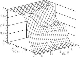
Figure 1: The $f$-level occupancy as a function of $\varepsilon_{f}$ and $U_{f}$ at half filling ($n=2$) for $V/W=0.1$.

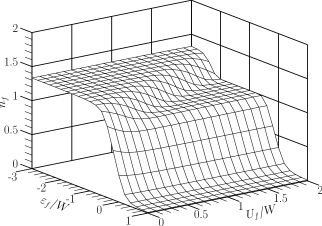
Figure 2: The $f$-level occupancy as a function of $\varepsilon_{f}$ and $U_{f}$ at 1/3 filling ($n=4/3$) for $V/W=0.1$.

The boundary of the $n_{f}\approx 1$ plateau could be defined by setting a somewhat arbitrary criterion for the deviation of $n_{f}$ from unity. Figure 3 shows $n_{f}$ in the $U_{f}$–$\varepsilon_{f}$ plane for a particular value of $V/W$ using a color code. The “boundary” of the plateau defined by $|1-n_{f}|=0.005$ is drawn with a white line. As can be seen in the figures, a plateau develops only when $U_{f}$ exceeds a not sharply defined threshold value, $U^{\text{c}}_{f}$, which itself depends on $V$ and on the total electron density. Besides $V/W=0.1$, we have done calculations for $V/W=0.05$ and $0.2$, and obtained similar results. The upper and lower limits of $\varepsilon_{f}$ between which the plateau forms can be estimated from the numerical data to be roughly

$$-U_{f}+E_{\rm F}(n_{d})+a\Delta_{f}\lesssim\varepsilon_{f}\lesssim E_{\rm F}(n_{d})-a\Delta_{f},$$ (9)

where $E_{\rm F}(n_{d})$ is the Fermi level of the conduction band with $n_{d}\!=\!n\!-\!1$ electrons, $\Delta_{f}=\pi\rho V^{2}$ is the width of the $f$-level in the impurity problem, and $a$ is a numerical factor of order 10, which depends weakly on $V$, $U_{f}$, and $n$. The factor $a$ is smaller by about $10\%$ for $n=4/3$ than for $n=2$, which shows that the plateau slightly expands as the filling of the conduction band decreases from half filling.

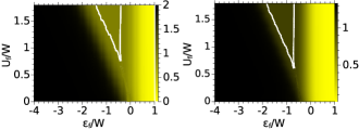
Figure 3: (Color online) The $f$-level occupancy as a function of $\varepsilon_{f}$ and $U_{f}$ at half filling (left) and 1/3 filling (right) for $V/W=0.1$. The color code is shown at the right edge of the panels. The boundary of the $n_{f}\approx 1$ plateau is drawn with a white line.

These results are somewhat surprising. One could argue, based on the results for the impurity Anderson model that a Kondo-like behavior (i.e., $n_{f}\approx 1$ with very small valence fluctuations) is realized when the Fermi level is located between the bare $f$-level ($\varepsilon_{f}$) and the energy $\varepsilon_{f}+U_{f}$ of a second $f$-electron occupying the same site. That is, we could expect the condition $-U_{f}+E_{\rm F}\lesssim\varepsilon_{f}\lesssim E_{\rm F}$, when $\Delta_{f}\ll W$. Condition (9) obtained by the Gutzwiller method indicates that the Kondo-like behavior is realized in the periodic Anderson model in a much narrower interval for $\varepsilon_{f}$. This will be confirmed later by exact diagonalization.

The $f$-electrons are strongly correlated on this plateau, since not only the average occupancy of the $f$-orbital is close to unity there, but the number of empty or doubly occupied $f$-orbitals is almost negligible. Correlations between $f$-electrons can conveniently be characterized by the renormalization factor $q_{f}$, which is simply related to the double-occupancy rate $\nu_{f}$ as

$$q_{f}=8\nu_{f}(1-2\nu_{f}),$$ (10)

when $n_{f}$ is exactly one. This quantity is plotted versus $\varepsilon_{f}$ and $U_{f}$ in Fig. 4 for $V/W=0.1$ at half filling.

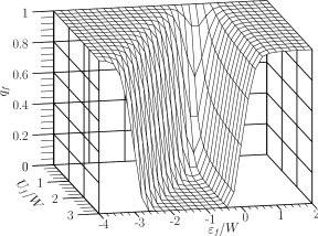
Figure 4: The kinetic energy renormalization factor of $f$-electrons as a function of $\varepsilon_{f}$ and $U_{f}$ at half filling for $V/W=0.1$.

It is clearly seen that $q_{f}$ decreases rapidly from about $1$, when the $f$-level is doubly occupied or empty, to about $0$ as $n_{f}$ approaches one from either side. When $q_{f}\approx 0$, the double-occupancy rate is also close to zero, and the $f$-electrons show heavy-fermion behavior; the effective mass becomes large as $m^{*}\propto q_{f}^{-1}$. We can, therefore, define the Kondo regime by setting a limit on $q_{f}$, by requiring, e.g., $q_{f}<0.005$. This boundary is marked by a white line in Fig. 5, where $q_{f}$ is shown for $n=2$ and $n=4/3$ using a color code.

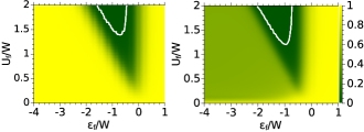
Figure 5: (Color online) The parameter $q_{f}$ is displayed for $V/W=0.1$ using a color code shown at the right edge. The boundary of the Kondo regime defined by $q_{f}=0.005$ is drawn with a white line. Left: half-filled case, right: 1/3-filled case.

The Kondo regime thus defined appears again above a critical $U_{f}^{\text{c}}$, which is, however, somewhat larger than the one found earlier, since the criterion $|1-n_{f}|\leq 0.005$ is less strict than the condition $q_{f}<0.005$. In this latter case the probability of double occupancy has to be less than $0.0006$. Nevertheless, comparison with Fig. 3 shows that apart from a rounding around the critical $U_{f}^{\text{c}}$, the two criteria define the same regime. The plateau slightly expands when the filling of the conduction band decreases.

When $n_{f}$ is exactly one, and Eq. (10) holds, Eq. (8) can be easily solved in the limit $V\ll W$. We get

$$q_{f}=\frac{n_{d}}{4(V/W)^{2}}\;\text{exp}\left(-\;\frac{U_{f}}{16V^{2}/W}\right),$$ (11)

where $n_{d}$ is the number of the conduction electrons per site. The factor $n_{d}$ in the prefactor explains why the critical $U^{\text{c}}_{f}$ gets smaller as the filling decreases.

The total energy density takes a simple form in this limit,

$${\mathcal{E}}=\varepsilon_{f}+E_{d}(n_{d})-n_{d}\frac{W}{2}\exp{\left\{-\frac{U_{f}}{16V^{2}/W}\right\}},$$ (12)

where the first term is the energy of the half-filled $f$-orbital without polarity fluctuations, $E_{d}(n_{d})$ is the energy of the decoupled conduction band for filling $n_{d}$, and the last term describes the coupling between $f$-electrons and conduction electrons, in other words, the energy decrease owing to the polarity fluctuations caused by $d$-$f$ hybridization. This term arising from the Kondo effect gives the characteristic energy scale in the Kondo regime. The Kondo energy, $E_{\text{K}}$, is defined by the energy decrease per conduction electron, i.e.,

$$E_{\text{K}}=\frac{W}{2}\exp{\left\{-\frac{U_{f}}{16V^{2}/W}\right\}}.$$ (13)

In the remaining part of this subsection, we study more quantitatively the dependence of the threshold value of $U_{f}^{\text{c}}$ on $V$ in the half-filled case. Figure 6 shows $q_{f}$ as a function of $V$ for several values of $U_{f}$ at $\varepsilon_{f}=-U_{f}/2$, where $n_{f}$ is exactly one.

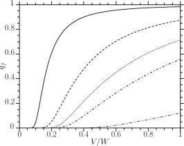
Figure 6: $q_{f}$ vs. $V$ in the symmetric half-filled case, $\varepsilon_{f}=-U_{f}/2$, for $U_{f}/W=1$ (continuous line), 3 (dashed), 5 (dotted), 7 (dashed with one dot), and 20 (dashed with two dots), respectively.

The threshold values determined from $q_{f}(U^{\text{c}}_{f},V)=0.005$ are given in Table 1 together the corresponding Kondo coupling $J=8V^{2}/U_{f}^{\text{c}}$, since, in the Kondo regime, the periodic Anderson model can be mapped onto a Kondo lattice model (KLM).

$V/W$	$U^{\text{c}}_{f}/W$	$J/W$
$0.16$	3	$0.066$
$0.21$	5	$0.071$
$0.26$	7	$0.076$
$0.48$	20	$0.093$
$0.74$	40	$0.110$
$0.97$	60	$0.125$
$1.17$	80	$0.136$
$1.36$	100	$0.148$

Table 1: The critical $U^{\text{c}}_{f}$ of the Kondo plateau for several values of $V$ and the corresponding Kondo coupling.

The dependence of $U^{\text{c}}_{f}$ on $V$ can be fitted by the analytic functional form

$$U^{\text{c}}_{f}/W=62.56(V/W)^{\alpha}.$$ (14)

with $\alpha=1.54$

Since by definition there are no doubly occupied or vacant $f$-orbitals in a KLM, a rigorous mapping from PAM to KLM should be possible in the limit $\nu_{f}\rightarrow 0$. Setting a smaller limit for $q_{f}$ in the criterion for the Kondo regime, larger exponents, given in Table 2, and larger numerical prefactors are obtained in Eq. (14). The exponent $\alpha$ seems to converge to 2 in the limit $q_{f}\rightarrow 0$, which means that $U_{f}^{\text{c}}$ is proportional to $\Delta_{f}$, and the proportionality factor is of order hundred instead of the factor $a\approx 10$ in Eq. (9). This difference is due to the stricter condition on $q$ and to the rounding of the boundary at the critical $U_{f}^{\text{c}}$.

$q_{f}^{\text{threshold}}$	$10^{-3}$	$10^{-4}$	$10^{-5}$	$10^{-6}$	$10^{-7}$	$10^{-8}$
$\alpha$	1.70	1.80	1.83	1.86	1.89	1.91

Table 2: The exponent $\alpha$ in Eq. (14) calculated for several threshold value of $q_{f}$.

Sinjukow and NoltingNolting:2002 have shown that in the extended Kondo limit, when $U_{f}\rightarrow\infty$ and $V\rightarrow\infty$ with $V^{2}/U_{f}$ remaining finite, the symmetric periodic Anderson model can be mapped exactly to the Kondo lattice model with finite Kondo coupling. The results obtained by the Gutzwiller method are in agreement with this.

II.2 Comparison with exact diagonalization

With the aim to compare the variational results with those of a completely different method, we also performed exact diagonalization on relatively short chains. In order to check whether the results obtained for these chains are representative for bulk materials, we calculated the $f$-level occupancy, $n_{f}$, and the density of doubly occupied $f$-sites, $\nu_{f}$, in the nonmagnetic ($S_{z}^{\rm tot}=0$) ground state for chains of four, five, and six sites. It turned out that the results were in excellent agreement with each other, which suggests that the six-site chain behaves almost like the bulk in this respect. This is in agreement with the finding of Chen and Callaway,Callaway:diag&MC who compared the ground-state energy obtained from exact diagonalization of a four-site chain with Monte Carlo result on a sixteen-site chain. In what follows we present the results obtained for a six-site chain with 12, 10, 8, and 6 electrons. The case with 6 electrons is not interesting from the point of view of Kondo physics, because the conduction band is exhausted when $n_{f}=1$. Nevertheless, it is used in the comparison of the two methods.

The kinetic energy of conduction electrons moving along the chain is described by hopping between nearest-neighbor $d$-orbitals with hopping rate $t$, thus the band width is now $4t$. Therefore, we identify $W$ with $4t$, when comparison with the results of the variational calculation is made.

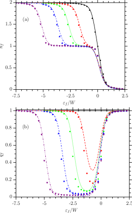
Figure 7: (Color online) (a) The $f$-level occupancy vs. $\varepsilon_{f}$ at $2V/W=0.375$. The curves are obtained by the Gutzwiller method, while the symbols indicate the results of exact diagonalization for $2U_{f}/W=0$ (black continuous line, •), 3 (red dashed line, $\blacksquare$), 5 (green dotted line, $\blacklozenge$), 7 (blue dashed line with one dot, $\blacktriangle$) and 10 (purple dashed line with two dots, $\blacktriangledown$). (b) The renormalization factor $q_{f}$. The notation is the same as in panel (a).

The $f$-level occupancy obtained by the two methods are directly compared in Fig. 7(a). As for $\nu_{f}$, we compare the results indirectly, through $q_{f}$. Although this quantity is specific to the Gutzwiller method, it shows the strength of correlations more visibly than $\nu_{f}$ itself, therefore, we define $q_{f}$ with the help of Eq. (5) from $n_{f}$ and $\nu_{f}$ obtained from the exact ground-state wave function. Comparison with the result of the variational calculation is shown in Fig. 7(b).

As is seen in Fig. 7(a), the two methods give very similar results as far as the “global behavior” of the $f$-level occupancy and the extent of the $n_{f}\approx 1$ plateau is concerned, even though the density of states is not identical in the two calculations. This indicates that Eq. (9) found in the Gutzwiller method for the boundary of the Kondo regime is not due to the Gutzwiller approximation, but is a consequence of strong correlations in the lattice model.

We find a subtle difference, however, in Fig. 7(b), where $q_{f}$ is plotted as a function of $\varepsilon_{f}$. One sees that $q_{f}$ calculated in the Gutzwiller method approaches zero faster in the Kondo regime than that provided by exact diagonalization. The former exhibits the exponential behavior given in Eqs. (11) and (13) typical for Kondo physics, while the latter cannot be fitted to such a curve. We will discuss this quantitatively later on.

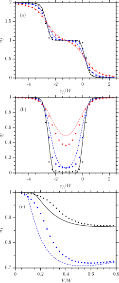
Figure 8: (Color online) (a) The $f$-level occupancy vs. $\varepsilon_{f}$ at $U_{f}/W=2.5$. The curves are obtained by the Gutzwiller method, while symbols denote the results of exact diagonalization for $2V/W=0.2$ (black continuous, •), $0.375$ (blue dashed, $\blacklozenge$), and $0.7$ (red dotted, $\blacksquare$), respectively. (b) The renormalization factor $q_{f}$. The notation is the same as in panel (a). (c) $n_{f}$ vs. $V$ at $U_{f}/W=2.5$, for $\varepsilon_{f}/W=-0.75$ (black continuous line, •) and $\varepsilon_{f}/W=-0.25$ (blue dashed line, $\blacksquare$).

Next we check the dependence of the Kondo plateau on the strength of the hybridization. In Fig. 8(a) we plot $n_{f}$ as a function of $\varepsilon_{f}$ for three values of $V/W$ in the half-filled case. It is clearly seen that the plateau (i.e., the Kondo regime) rapidly shrinks as $V$ increases, and disappears, in agreement with the results presented in the previous subsection. Figure 8(b), where $q_{f}$ is plotted, shows directly the disappearance of heavy-fermion behavior. Finally $n_{f}$ is plotted as a function of $V$ in Fig. 8(c) for two values of $\varepsilon_{f}/W$. We find again that the two methods yield similar results for $n_{f}$, but the $V$-dependence is different near the boundary of the Kondo regime.

In order to better see this difference, we calculate the double-occupancy rate of $f$-electrons in the symmetric ($\varepsilon_{f}=-U_{f}/2$) half-filled case as a function of $V$ near the boundary of the Kondo regime, i.e., where $\nu_{f}\ll 1$. We find, as seen in Fig. 9, that in contrast to the results of the Gutzwiller method, the dependence of $\nu_{f}$ on $V^{2}/U_{f}$ is not exponential; $\nu_{f}$ varies as a power of $V^{2}/U_{f}$:

$$\nu_{f}=A\;\frac{W}{U_{f}}\left(\frac{V^{2}}{WU_{f}}\right)+B\;\frac{W}{U_{f}}\left(\frac{V^{2}}{WU_{f}}\right)^{2},$$ (15)

where $A$ is close to unity and $B\approx 50$. This power-law-like dependence may be due to the small system size in the exact diagonalization.

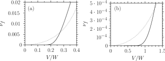
Figure 9: The double-occupancy rate of $f$-electrons vs. $V/W$. The dotted curves indicate the results of exact diagonalization, while the continuous curves are calculated by the Gutzwiller method. $U_{f}/W$ is 5 and 100 in panel (a) and (b), respectively.

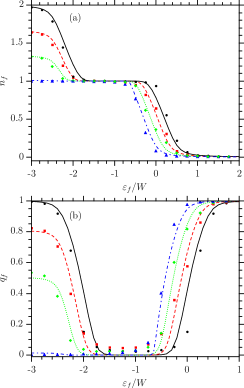
Figure 10: (Color online) (a) The $f$-level occupancy vs. $\varepsilon_{f}$ at $U_{f}/W=2$ for different fillings. The hybridization is $V/W=0.1$ in all cases. The curves are obtained by the Gutzwiller method, while the symbols are the results of exact diagonalization. The number of electrons per site is $n=2$ (black continuous line, •), 5/3 (red dashed line, $\blacksquare$), 4/3 (green dotted line, $\blacklozenge$), 1 (blue dashed line with one dot, $\blacktriangle$), respectively. (b) The $f$-level kinetic energy renormalization factor. The notation is the same as in panel (a).

Finally we study the filling dependence of the Kondo regime. The $f$-level occupancy is shown for several fillings in Fig. 10(a). The overall agreement between the two methods persists as we move away from half filling, though its degree varies somewhat, e.g., the agreement in the $n=2$ or 5/3 case is noticeably less good than for $n=4/3$. This indicates that the Gutzwiller type paramagnetic wave function is more appropriate for metallic systems with few conduction electrons than for insulators. The Kondo plateau shifts towards lower $f$-level energies as the filling decreases owing to the decrease of the Fermi level. We find a similar slight difference between the results of the two methods displayed in Fig. 10(b), where $q_{f}$ is plotted as a function of $\varepsilon_{f}$.

III The role of interaction between conduction electrons

III.1 Variational calculation

As a next step, we consider what happens when the interaction between conduction electrons is switched on. For the sake of simplicity a local, on-site interaction is assumed and the Hamiltonian takes the form

$$\mathcal{H}=\mathcal{H}_{\textrm{PAM}}+U_{d}\sum_{j}\hat{n}^{d}_{j\uparrow}\hat{n}^{d}_{j\downarrow}\;,$$ (16)

where $\mathcal{H}_{\textrm{PAM}}$ is the PAM Hamiltonian defined in Eq. (1) and $U_{d}$ is the strength of the Coulomb interaction between conduction electrons. This model is also known as the periodic Anderson-Hubbard model. At half filling the symmetric model corresponds to $\varepsilon_{f}=-U_{f}/2+U_{d}/2$, where $n_{f}=n_{d}=1$.

The variational calculation can be performed by a simple generalization of the procedure used for $U_{f}\rightarrow\infty$.Itai:variational The trial wave function is chosen in the form

$$|\Psi\rangle=\hat{P}_{\text{G}}^{f}\hat{P}_{\text{G}}^{d}\prod_{\boldsymbol{k}}\prod_{\sigma}\left[u_{\boldsymbol{k}}\hat{f}_{\boldsymbol{k}\sigma}^{\dagger}+v_{\boldsymbol{k}}\hat{d}_{\boldsymbol{k}\sigma}^{\dagger}\right]|0\rangle,$$ (17)

where $\hat{P}^{f}_{\text{G}}$ contains the variational parameter $\eta_{f}$, and an extra Gutzwiller projector has been introduced for $d$-electrons, which is written as

$$\hat{P}_{\text{G}}^{d}=\prod_{\boldsymbol{j}}\left[1-(1-\eta_{d})\hat{n}_{j\uparrow}^{d}\hat{n}_{j\downarrow}^{d}\right].$$ (18)

The variational parameter $\eta_{d}$ depends on $U_{d}$. Performing the optimization with respect to the mixing amplitudes we get

$$\mathcal{E}=\frac{1}{N}\sum_{\boldsymbol{k}\in\mathrm{FS}}\left[q_{d}\varepsilon_{d}(\boldsymbol{k})+\tilde{\varepsilon}_{f}-\sqrt{\big{[}q_{d}\varepsilon_{d}(\boldsymbol{k})-\tilde{\varepsilon}_{f}\big{]}^{2}+4\tilde{V}^{2}}\right]$$

$$+(\varepsilon_{f}-\tilde{\varepsilon}_{f})n_{f}+U_{d}\nu_{d}+U_{f}\nu_{f}$$ (19)

for the ground-state energy density, where $\nu_{d}$ is the density of doubly occupied $d$-sites, and $q_{d}$ denotes the kinetic energy renormalization factor of $d$-electrons given by

$$q_{d} = \frac{1}{\left(1-\frac{n_{d}}{2}\right)\frac{n_{d}}{2}}\Bigg{[}\sqrt{\left(\frac{n_{d}}{2}-\nu_{d}\right)\nu_{d}}$$ (20)

$$+\sqrt{\left(\frac{n_{d}}{2}-\nu_{d}\right)(1-n_{d}+\nu_{d})}\;\Bigg{]}^{2},$$

which is formally identical to that found in the Hubbard model.Gutzwiller:original The renormalized hybridization amplitude is now $\tilde{V}=V\sqrt{q_{d}q_{f}}$; the other notations are the same as in the previous section, and the self-consistency condition [see Eq. (6)] is now given by

$$n_{f}=\frac{1}{N}\sum_{\boldsymbol{k}\in\mathrm{FS}}\left[1+\frac{q_{d}\varepsilon_{d}(\boldsymbol{k})-\tilde{\varepsilon}_{f}}{\sqrt{\big{[}q_{d}\varepsilon_{d}(\boldsymbol{k})-\tilde{\varepsilon}_{f}\big{]}^{2}+4{\tilde{V}}^{2}}}\right].$$ (21)

The summation over $\boldsymbol{k}$ and the numerical optimization of the energy density with respect to $n_{f}$, $\nu_{f}$, and $\nu_{d}$ are carried out in the same way as in the previous section. The equations determining $n_{f}$, $\nu_{f}$ and $\nu_{d}$ are now

$${\tilde{\varepsilon}}_{f} = \frac{\partial{\cal E}}{\partial q_{d}}\cdot\frac{\partial q_{d}}{\partial n_{f}}+\frac{\partial{\cal E}}{\partial q_{f}}\cdot\frac{\partial q_{f}}{\partial n_{f}}+\frac{\partial{\cal E}}{\partial{\tilde{\varepsilon}}_{f}}\cdot\frac{\partial{\tilde{\varepsilon}}_{f}}{\partial n_{f}},$$ (22)

$$-U_{f} = \frac{\partial{\cal E}}{\partial q_{f}}\cdot\frac{\partial q_{f}}{\partial{\nu_{f}}}+\frac{\partial{\cal E}}{\partial{\tilde{\varepsilon}}_{f}}\cdot\frac{\partial{\tilde{\varepsilon}}_{f}}{\partial\nu_{f}},$$ (23)

$$-U_{d} = \frac{\partial{\cal E}}{\partial q_{d}}\cdot\frac{\partial q_{d}}{\partial{\nu_{d}}}+\frac{\partial{\cal E}}{\partial{\tilde{\varepsilon}}_{f}}\cdot\frac{\partial{\tilde{\varepsilon}}_{f}}{\partial\nu_{d}}.$$ (24)

First we derive analytic results from these equations in the weak hybridization limit up to $O((V/W)^{2})$ for arbitrary $U_{f}$ at special fillings: for $n_{f}=1$ and $n_{d}$ arbitrary; for $n_{d}=1$ and $n_{f}$ arbitrary; and finally for $n_{f}=n_{d}=1$. Similar results were obtained in Ref. [Itai:variational, ], but only for $U_{f}\rightarrow\infty$.

We know that the interaction between conduction electrons suppresses charge fluctuations in the Hubbard subsystem. This influences the Kondo physics in the following ways:

(i) $U_{d}$ shifts the Fermi energy of the conduction band. For $n_{f}=1$ and $n_{d}<1$ we get

$$E_{\text{F}}(n_{d},U_{d})\approx\left(\frac{n_{d}}{2}-\frac{1}{2}\right)q_{d}W\;\;\;\;\;\;\;\;\;\;\;\;\;\;\;\;\;\;\;\;\;\;\;\;\;\;\;\;\;\;\;\;\;\;$$

$$\;\;\;\;\;+\;W\left[-\frac{1}{4}+\left(\frac{n_{d}}{2}-\frac{1}{2}\right)^{2}-2\left(\frac{V}{W}\right)^{2}\frac{q_{f}}{q_{d}}\right]\frac{\partial q_{d}}{\partial n_{d}}.$$ (25)

The third term in the square brackets is the contribution of $d$-$f$ hybridization. Without it we recover the equation determining the Fermi energy of the Hubbard model for filling $n_{d}$. Note that the values of $\nu_{f}$ and $\nu_{d}$ in $q_{f}$ and $q_{d}$, respectively, should be taken from the solution of Eqs. (23) and (24). Equation (25) has no simple closed form solution for arbitrary $U_{d}$ except for the half-filled case, where $E_{\text{F}}(n_{d}=1,U_{d})=U_{d}/2$. At other fillings we can expand $E_{\text{F}}(n_{d},U_{d})$ in the weak- or strong-coupling limit ($U_{d}\ll W$ or $U_{d}\gg W$) as

$$E_{\text{F}}(n_{d},U_{d})\approx E_{\text{F}}(n_{d},0)+\frac{n_{d}}{2}U_{d}+O(U_{d}^{2}/W)$$ (26)

or

$$E_{\text{F}}(n_{d},U_{d})\approx E_{\text{F}}(n_{d},0)+\frac{n_{d}}{2}W+O(W^{2}/U_{d}),$$ (27)

respectively. The shift of the Fermi energy is at most $W/6$ for $n=4/3$ (i.e., $n_{d}=1/3$), which is much smaller than the shift in the half-filled case.

(ii) Switching on $U_{d}$ reduces the Kondo energy.Itai:variational When $n_{f}=1$, we can calculate $q_{f}$ and the total energy density for finite $U_{d}$ and for arbitrary $n_{d}$ (assuming $V\ll W$). Instead of Eqs. (11) and (12) we find

$$q_{f}=\frac{n_{d}q_{d}}{4(V/W)^{2}}\;\exp\left(-\frac{U_{f}}{16V^{2}/W}\right),$$ (28)

and

$${\mathcal{E}}=\varepsilon_{f}+E_{d}(n_{d},U_{d})-n_{d}q_{d}\frac{W}{2}\exp{\left\{-\frac{U_{f}}{16V^{2}/W}\right\}},$$ (29)

where the second term of the right hand side is the energy of the decoupled correlated conduction band. Compared with Eqs. (11) and (13), $q_{f}$ and the exponential Kondo scale are reduced by $q_{d}$, which is rather small when $n_{d}\approx 1$ (see below). For $n$ slightly less than the half-filled case this mechanism yields a significant mass enhancement. We get $q_{d}\sim 1/5$ for $n=1.95$ and $U_{d}=2.4W$, which means that the effective mass is five times bigger for these parameters than without $U_{d}$.

(iii) The most interesting effect of $U_{d}$ is the Mott transition which occurs in the Hubbard model at half filling ($n_{d}=1$). In the Gutzwiller-type treatment of $U_{d}$ it is known as the Brinkman-Rice transition. It occurs when $q_{d}$ becomes zero for a finite $U_{d}$. A similar transition may take place in the half-filled periodic Anderson-Hubbard model. In this model, however, even if $n=2$, the Kondo physics may compete with Mott physics, $n_{d}$ and $n_{f}$ depend on $U_{d}$, $U_{f}$, $V$, and $\varepsilon_{f}$ owing to the $d$-$f$ hybridization, and the conditions for the Mott transition may not be so simple as in the Hubbard model. In what follows we first show in the framework of the Gutzwiller treatment that the necessary conditions for the Mott transition is that both the $f$- and $d$-electron subsystem be half filled, i.e., $n_{d}=1$ and $n_{f}=1$ be fulfilled simultaneously, and moreover the system be in the Kondo regime.

We see from Eq. (20) that $q_{d}$ is zero only when $n_{d}=1$ and $\nu_{d}=0$. Similarly it follows from Eq. (5) that $q_{f}$ vanishes only if $n_{f}=1$ and $\nu_{f}=0$. When $n_{d}=1$, the renormalization factor $q_{d}$ is simply $8\nu_{d}(1-2\nu_{d})$, and Eq. (24) gives

$$\frac{U_{d}}{W}-\left[\frac{1}{4}+2\left(\frac{V}{W}\right)^{2}\frac{q_{f}}{q_{d}}\right]8(1-4\nu_{d})=0$$ (30)

for $V\ll W$ and $n_{f}$ arbitrary. The second term in the square brackets is the contribution of $d$-$f$ hybridization. Without it we recover the equation determining the optimum $\nu_{d}$ of the half-filled Hubbard model.

It follows from this equation that $\nu_{d}$ goes to zero as $U_{d}$ approaches a finite critical value only if $q_{f}$ also approaches zero, and $q_{f}$ is of the same order as $q_{d}$. This situation can be realized only if $n_{d}=1$ and $n_{f}=1$ are simultaneously fulfilled, and moreover $q_{f}$ is given by Eq. (28), i.e., the system is in the Kondo regime.

When $n_{d}=1$ and $n_{f}=1$ are simultaneously satisfied, and the system is in the Kondo regime, the term in (30) due to $d$-$f$ hybridization is independent of $\nu_{d}$ and is equal to $E_{\text{K}}/W$ [see Eqs. (13), (28), and (29)]. Equation (30) is easily solved to give

$$\nu_{d}=\frac{1}{4}-\frac{U_{d}}{8(W+4E_{\text{K}})},$$ (31)

which shows that $\nu_{d}$ decreases linearly as $U_{d}$ increases and reaches zero at $U_{d}^{\text{c}}=2(W+4E_{\text{K}})$. At this value of $U_{d}$, which – owing to the coupling between the $d$- and $f$-electron subsystems – is slightly larger than the critical value in the Hubbard model ($U_{d}^{\text{c}}=2W$), the conduction band undergoes a Brinkman-Rice transition. Note that the exponentially small correction has been neglected in Ref. [Itai:variational, ]. Since $\nu_{d}=\nu_{f}=0$ at this transition, all polarity fluctuations are suppressed, the effective $d$-$f$ hybridization ($\tilde{V}=V\sqrt{q_{d}q_{f}}$) as well as the Kondo energy scale become zero, that is, the Kondo effect is completely quenched. The system transforms from a Kondo insulator into a Mott insulator.

Analytically we can claim only that the condition $n_{d}=n_{f}=1$ is realized in the symmetric point of the half-filled model, where $\varepsilon_{f}=-U_{f}/2+U_{d}/2$. Indeed, when $U_{d}$ is smaller than $U_{d}^{\text{c}}$ and is not very close to it, it is found numerically that $n_{d}=n_{f}=1$ is realized only at the symmetric point, and thus one could expect that a Brinkman-Rice transition occurs only in the half-filled symmetric periodic Anderson-Hubbard model, and that the system becomes a Mott insulator for $U_{d}>U^{\text{c}}_{d}$ only if $\varepsilon_{f}=-U_{f}/2+U_{d}/2$.

Contrary to this expectation we have found numerically that when $U_{d}$ is slightly smaller than the critical value, $n_{f}=n_{d}=1$ holds not only at the symmetric point, but – within the limits of the numerical accuracy of our calculations, which was about $10^{-6}$ – in a wide range of $\varepsilon_{f}$ within the $n_{f}\approx 1$ plateau. In order to find the extent of this range, we display the $U_{d}$- and $\varepsilon_{f}$-dependence of the $f$-level occupancy and of the renormalization factor $q_{f}$ for $U_{d}\leq 2W$ at half filling in Figs. 11 and 12, respectively.

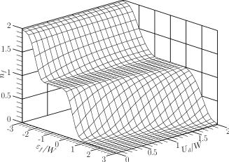
Figure 11: The $f$-level occupancy vs. the $f$-level energy and $U_{d}$ at half filling for $V/W=0.1$ and $U_{f}/W=2$.

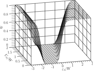
Figure 12: The kinetic energy renormalization factor for $f$-electrons vs. $\varepsilon_{f}$ and $U_{d}$ at half filling for $V/W=0.1$ and $U_{f}/W=2$.

It is clearly seen that the Kondo plateau, where $n_{f}\approx 1$ and $q_{f}\approx 0$, shifts towards higher energies owing to the shift of the Fermi energy by $U_{d}/2$, and the center of the plateau is located indeed at $\varepsilon_{f}=-U_{f}/2+U_{d}/2$ as expected from Eq. (25). The condition for the Kondo regime can be written similarly to Eq. (9) as

$$-U_{f}+E_{\text{F}}(n_{d},U_{d})+a\Delta_{f}\lesssim\varepsilon_{f}\lesssim E_{\text{F}}(n_{d},U_{d})-a\Delta_{f}.$$ (32)

Note that the center of the plateau is at the center of the noninteracting $d$-band, when $U_{d}=U_{f}$. In other words, the $f$-level does not need to lie low enough compared to the conduction band to show heavy-fermion behavior.

Another remarkable feature is that the plateau widens as $U_{d}$ approaches the critical value $U_{d}^{\text{c}}$. At $U_{d}=2W$, it is situated in the range $-U_{f}+U_{d}/2\lesssim\varepsilon_{f}\lesssim U_{d}/2$. That means that the narrowing of the plateau compared to the impurity model given by $a\Delta_{f}$ in Eq. (9) gets remarkably smaller close to $U_{d}^{\text{c}}$. This is probably due to the formation of the Hubbard subbands and the drastic variation of the density of states at the Fermi energy near the transition point.

Numerical calculations give $n_{d}=n_{f}=1$ at $U_{d}^{\text{c}}$ on the whole Kondo plateau. This indicates that – at least within the Gutzwiller-type treatment of correlations – both $n_{d}$ and $n_{f}$ are fixed to exactly unity in the half-filled model as we approach $U_{d}^{\text{c}}$ and the condition for Kondo behavior is satisfied. The renormalization factors, $q_{d}$ and $q_{f}$ vanish simultaneously, the $d$-$f$ hybridization is completely suppressed, so is the Kondo effect, and a Mott transition takes place. This transition in the conduction electron subsystem is robust, it is the dominant feature of the half-filled model.

Our finding that the Brinkman-Rice transition and the Mott insulating state are not restricted to the symmetric model is corroborated by calculations for $U_{d}>U^{\text{c}}_{d}$. The numerical variational calculation yields meaningless negative values for $\nu_{d}$ in the whole interval $-U_{f}+U_{d}/2\lesssim\varepsilon_{f}\lesssim U_{d}/2$. Note that for $\varepsilon_{f}$ outside this interval we can carry out the numerical calculations for arbitrary large $U_{d}$ without any difficulty.

Next we show that the $d$-$f$ hybridization prevents the Mott transition when $n<2$ (or for $n>2$). In this case the term coming from the $d$-$f$ hybridization in Eq. (30) becomes large, if $q_{d}\rightarrow 0$, since $q_{f}$ is always finite for $n_{f}<1$, and thus there exists no such solution for $\nu_{d}$ (or $q_{d}$), which approaches zero at a finite $U_{d}$. Charge fluctuations on the $d$-orbitals are thus not completely suppressed. A finite $\nu_{d}$ indicates the existence of a Fermi surface, since $q_{d}$ is identified with the discontinuity at the Fermi wavenumber in the single-particle occupation number.Gutzwiller:original This can be understood as follows: even if the correlated conduction band is half filled and $U_{d}$ is large enough, so that the conduction band is separated into Hubbard subbands and the Fermi level lies within the $f$-band located in the Hubbard gap, the $d$-electrons are taking part in the formation of the Fermi surface via $d$-$f$ hybridization.

The results of the numerical calculations in the 1/3-filled case ($n=4/3$) are shown for $0\leq U_{d}\leq 3W$ in Fig. 13. We observe that one more plateau appears at higher $f$-level energies, above the bare conduction band, when $U_{d}\gtrsim 2W$, corresponding to $n_{d}\approx 1$. Its formation indicates that two separate Hubbard subbands are formed above this critical value of $U_{d}$. The plateau appears when $\varepsilon_{f}$ is located between the two subbands, i.e., in the Hubbard gap. The Fermi level is located in the $f$-band in this situation. The center of the plateau is approximately at $U_{d}/2$, which indicates that the upper and lower subbands are centered at 0 and $U_{d}$, respectively, i.e., the location of the subbands is the same as in the Hubbard model.

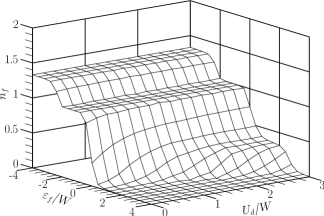
Figure 13: The $f$-level occupancy vs. $f$-level energy and $U_{d}$ at 1/3 filling ($n=4/3$), for $V/W=0.1$ and $U_{f}/W=2$.

We observe furthermore that the $n_{f}\approx 1$ plateau hardly shifts as $U_{d}$ increases. Since according to Eq. (27) the Fermi energy only weakly depends on $U_{d}$ away from half filling, we find again the condition given in (32) for the Kondo regime.

It is worth mentioning here what happens when the system is more than half filled. The answer can be obtained without any further calculation from electron-hole symmetry. A model with $n$ electrons can be mapped onto a model with $n$ holes ($4-n$ electrons) by the transformation:

$$\hat{d}_{j\sigma}^{\dagger}\rightarrow e^{i\varphi_{j}}\hat{d}_{{\text{h}}j\bar{\sigma}},\;\;\;\;\hat{d}_{j\sigma}\rightarrow e^{-i\varphi_{j}}\hat{d}^{\dagger}_{{\text{h}}j\bar{\sigma}},$$

$$\hat{f}_{j\sigma}^{\dagger}\rightarrow-e^{i\varphi_{j}}\hat{f}_{{\text{h}}j\bar{\sigma}},\;\;\;\;\hat{f}_{j\sigma}\rightarrow-e^{-i\varphi_{j}}\hat{f}^{\dagger}_{{\text{h}}j\bar{\sigma}},$$ (33)

where the index (h) refers to holes, and $\bar{\sigma}=-\sigma$. If the kinetic energy of conduction electrons is written in Wannier representation,

$$\sum_{\boldsymbol{k},\sigma}\varepsilon_{d}(\boldsymbol{k})\hat{d}_{\boldsymbol{k}\sigma}^{\dagger}\hat{d}^{\phantom{\dagger}}_{\boldsymbol{k}\sigma}=\sum_{ij\sigma}t_{ij}\hat{d}_{i\sigma}^{\dagger}\hat{d}^{\phantom{\dagger}}_{j\sigma},$$ (34)

and the phase factor is chosen in the form $\varphi_{j}=\boldsymbol{Q}\cdot{\boldsymbol{r}}_{j}$, it is easily seen that the kinetic energy term is transformed into

$$\sum_{\boldsymbol{k},\sigma}\varepsilon_{\text{h}d}(\boldsymbol{k})\hat{d}_{{\text{h}}\boldsymbol{k}\sigma}^{\dagger}\hat{d}^{\phantom{\dagger}}_{{\text{h}}\boldsymbol{k}\sigma},$$ (35)

where

$$\varepsilon_{\text{h}d}(\boldsymbol{k})=-\varepsilon_{d}(\boldsymbol{k}+{\boldsymbol{Q}}).$$ (36)

Assuming that $t_{ii}=0$, the center of the band sets the zero of energy. The term describing hybridization is invariant under this transformation, while the on-site energy of $f$-levels and the on-site interaction terms give rise to energy shifts. Therefore the Hamiltonian written in terms of the creation and annihilation operators of holes has the same form as for electrons with shifted energies for the $d$- and $f$-electrons, and an overall energy shift:

$${\mathcal{H}}_{\text{e}}\left(\varepsilon_{d}(\boldsymbol{k}),\varepsilon_{f},V,U_{d},U_{d}\right)\longrightarrow\;\;\;\;\;\;\;\;\;\;\;$$

$${\mathcal{H}}_{\text{h}}\left(\varepsilon_{\text{h}d}({\boldsymbol{k}})-U_{d},\;\varepsilon_{\text{h}f},V,U_{d},U_{f}\right)+E_{0},$$ (37)

where $\varepsilon_{\text{h}f}=-\varepsilon_{f}-U_{f}$ and $E_{0}=(2\varepsilon_{f}+U_{f}+U_{d})N$. If the energy levels are measured from $-U_{d}$ the Hamiltonian in hole representation becomes

$${\mathcal{H}}_{\text{h}}\left(\varepsilon_{\text{h}d}({\boldsymbol{k}}),\;\bar{\varepsilon}_{\text{h}f},V,U_{d},U_{f}\right)+\bar{E}_{0},$$ (38)

with $\bar{\varepsilon}_{\text{h}f}=-\varepsilon_{f}-U_{f}+U_{d}$ and

$$\bar{E}_{0}=-(2\varepsilon_{d}+U_{d})N_{\text{h}}+(2\varepsilon_{f}+U_{f}+2\varepsilon_{d}+U_{d})N,$$ (39)

where $N_{\text{h}}$ is the total number of holes. Provided that $\varepsilon_{\text{h}d}({\boldsymbol{k}})\equiv-\varepsilon_{d}({\boldsymbol{k}}+\boldsymbol{Q})=\varepsilon_{d}({\boldsymbol{k}})$ for a certain ${\boldsymbol{Q}}$, as is the case for the one-dimensional model with nearest-neighbor hopping, or when a constant density of states is assumed, then the dispersion curve of $d$-holes is the same as for $d$-electrons and the results obtained in the electron representation can be applied to holes when the energy shifts are taken into account.

Using this transformation, the results for $n>2$ can be obtained straightforwardly from those for $n_{\text{h}}=4-n<2$. We can get, for example, the Fermi energy of the correlated conduction band for $n_{d}=n-1>1$ ($n_{f}=1$) from that for $n_{\text{h}d}=2-n_{d}<1$ [see Eq. (25)] by first shifting the origin of the energy by $-U_{d}$, and then reversing the energy axis. We get

$$E_{\text{F}}(n_{d},U_{d})=-\big{[}E_{\text{F}}(n_{\text{h}d},U_{d})-U_{d}\big{]},$$ (40)

from which for $n_{d}>1$

$$E_{\text{F}}(n_{d},U_{d}=0)=-E_{\text{F}}(2-n_{d},U_{d}=0).$$ (41)

The equation giving the shift of the Fermi energy for $n_{d}>1$ is thus

$$E_{\text{F}}(n_{d},U_{d})\approx E_{\text{F}}(n_{d},0)-\frac{2-n_{d}}{2}W+U_{d}+O(W^{2}/U_{d})$$ (42)

instead of Eq. (27). This shows that the shift of the Fermi energy owing to $U_{d}$ for $n_{d}>1$ is larger than that at half-filling.

The condition on $\varepsilon_{f}$ for the Kondo regime is obtained for $n>2$ as follows: The condition on the $f$-hole level $\bar{\varepsilon}_{\text{h}f}$ for $n_{\text{h}}<2$ is formally the same as for electrons [see Eq. (32)], since the Hamiltonian has the same form, i.e.,

$$-U_{f}+E_{\text{F}}(n_{\text{h}d},U_{d})+a\Delta_{f}\lesssim\bar{\varepsilon}_{\text{h}f}\lesssim E_{\text{F}}(n_{\text{h}d},U_{d})-a\Delta_{f}.$$ (43)

The condition on the $f$-electron level for the Kondo regime for $n>2$ is simply obtained by rewriting this condition for the original $\varepsilon_{f}$ using $\bar{\varepsilon}_{\text{h}f}=-\varepsilon_{f}-U_{f}+U_{d}$. We get

$$-U_{f}+U_{d}-E_{\text{F}}(n_{\text{h}d},U_{d})+a\Delta_{f}\lesssim\;\;\;\;\;\;\;\;\;\;\;\;\;\;\;\;\;\;\;\;\$$

$$\;\;\;\;\;\;\;\;\;\;\varepsilon_{f}\lesssim U_{d}-E_{\text{F}}(n_{\text{h}d},U_{d})-a\Delta_{f}.$$ (44)

Since according to Eq. (40) $U_{d}-E_{\text{F}}(n_{\text{h}d},U_{d})$ ($n_{\text{h}d}<1$) is the Fermi energy of the interacting conduction band, $E_{\text{F}}(n_{d},U_{d})$, for $n_{d}=2-n_{\text{h}d}>1$, the condition takes the same form given in Eq. (32) for all fillings. For $n>2$, the shift of the $n_{f}\approx 1$ plateau is thus even larger than in the half-filled case, it may appear above the bare conduction band.

III.2 Comparison with the results by exact diagonalization

Now, we compare the results of exact diagonalization with those obtained by variational calculation. Note that we will discuss only the case $n>1$, i.e., more than six electrons on a six-site chain. The quarter-filled case is not interesting from the point of view of Kondo physics, because the conduction band is exhausted when $n_{f}=1$.

The values of $n_{f}$ obtained by both methods are shown for several fillings at $U_{f}=U_{d}=2W$ in Fig. 14(a). The overall agreement between the results of the two methods demonstrated earlier remains good for finite $U_{d}$. It is remarkable that the agreement is even better than for $U_{d}=0$.

The shift of the $n_{f}\approx 1$ plateau due to $U_{d}$ is observed in both methods, showing that the shift of the plateau is not an artefact of the Gutzwiller approximation, and may be observable in some materials, where the conduction electrons are strongly correlated, i.e., they may exhibit heavy-fermion behavior despite the fact that the bare $f$-level does not lie below the conduction band.

The formation of two separate plateaus corresponding to $n_{f}\approx 1$ and $n_{d}\approx 1$ is also observed in both methods. The formation of the Hubbard subbands owing to $U_{d}$ in the conduction-electron subsystem is thus confirmed by exact diagonalization, too. We carried out the comparison also at $U_{f}=U_{d}=5W$ for $n=5/3$, and found that the agreement between the two methods is almost perfect for $n_{f}$.

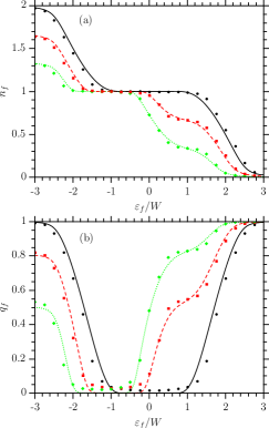
Figure 14: (Color online) (a) The $f$-level occupancy vs. $\varepsilon_{f}$ at $U_{f}/W=U_{d}/W=2$ and $V/W=0.1$. The curves are obtained using the Gutzwiller method, while the symbols are the results of exact diagonalization. The electron number per site is 2 (half filling) (black continuous line, •), 5/3 (red dashed line, $\blacksquare$), and 4/3 (green dotted line, $\blacklozenge$), respectively. (b) The renormalization factor $q_{f}$. The notation is the same as in panel (a).

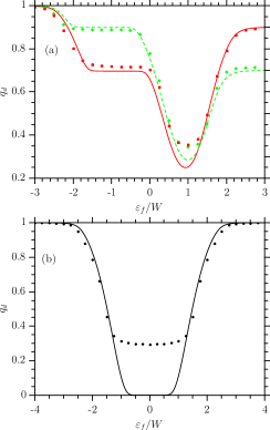
Figure 15: (Color online) The kinetic energy renormalization factors of the conduction electrons vs. $\varepsilon_{f}$ at $U_{f}/W=U_{d}/W=2$. The curves are obtained by the Gutzwiller method, the symbols show the values calculated with exact diagonalization using Eq. (20). (a) The results for $n=5/3$ (the red dashed line, $\blacksquare$) and $n$=4/3 (the green dotted line, $\blacklozenge$). The hybridization is $V/W=0.1$ in all cases. (b) The results for half filling, $n=2$ (the black continuous line, •).

Figure 15 shows the kinetic energy renormalization factor of conduction electrons ($q_{d}$) for three different fillings. The agreement between the two methods are fairly good in panel (a), while a marked difference is seen in panel (b), i.e., at half filling. At this point we should note that the two methods are complementary. The Gutzwiller method is exact for large dimensions, while the exact diagonalization was performed on chains. We argue that the difference between the results obtained by the two methods at half filling is due to the unusual behavior of the one-dimensional half-filled Hubbard model.

The one-dimensional Hubbard model can be solved exactly by Bethe ansatz.Lieb-Wu At half filling its ground state is conducting only for $U_{d}=0$ and insulating for any nonzero $U_{d}$. On the other hand, in higher dimensions the half-filled Hubbard model is expected to remain metallic until a finite critical $U_{d}^{\text{c}}$, where the Mott transition takes place. Therefore, when we compare the results obtained by the Gutzwiller method and by exact diagonalization of the Hamiltonian of a chain displayed in Fig. 15(b) and interpret the difference, we have to keep in mind the fundamental difference between the physics of one- and higher dimensional half-filled Hubbard models.

The Gutzwiller method gives not only a vanishing valence fluctuation on $f$-orbitals, $\nu_{f}=0$, and consequently $q_{f}=0$ at $U_{d}=2W+8E_{\text{K}}$, but the same is true for the conduction-electron subsystem: also $\nu_{d}$ and $q_{d}$ vanish at the Brinkman-Rice transition. On the other hand, exact diagonalization gives a finite $q_{d}$ in agreement with the known behavior of the one-dimensional half-filled Hubbard model, where $\nu_{d}$ is finite for arbitrary $U_{d}$.Woynarovich We believe that the disagreement between the predictions of the Gutzwiller method and of exact diagonalization seen in Fig. 15(b) is thus the consequence of the different behavior of the one-dimensional and higher dimensional periodic Anderson-Hubbard models.

IV Conclusions

In this paper we considered an extended periodic Anderson modell, the so-called periodic Anderson-Hubbard model with on-site Coulomb repulsion in the conduction-electron subsystem. Our main aim was to investigate how the additional repulsive interaction between conduction electrons influences the Kondo regime, and how the Kondo physics and Mott physics compete. For this study we calculated the average number of $f$- and $d$-electrons per site, $n_{f}$ and $n_{d}$, and the probability of double occupancy in both subsystems, $\nu_{f}$ and $\nu_{d}$, using the Gutzwiller variational method. In order to check the reliability of this method, we also performed exact diagonalization on relatively short chains. Since to our best knowledge no such comparison was presented even for the original periodic Anderson model, we also present results for the original periodic Anderson model.

A rather good agreement was found between the results of the two methods in the original model as far as the location of the Kondo and valence-fluctuation regimes are concerned. A subtle difference was, however, found near the boundary of the Kondo plateau. Namely, while the results of the Gutzwiller method exhibit an exponential dependence of the double occupancy on the characteristic combination of the couplings, $V^{2}/U_{f}$, those of exact diagonalization show a power-law behavior. This will be the subject of subsequent studies.

The situation is somewhat different for the extended model. Both methods indicate that when the on-site Coulomb repulsion between conduction electrons ($U_{d}$) is switched on, in the half-filled case the heavy-fermion regime shifts towards higher energies of the bare $f$-level by $U_{d}/2$ in accordance with the shift of the Fermi energy owing to $U_{d}$. A marked difference appears, however, between the results provided by the two methods, when $U_{d}$ is of the order of $2W$. The Gutzwiller method indicates that both $n_{d}$ and $n_{f}$ are fixed to unity for a wide range of the $f$-level energies in the half-filled model at a critical value of $U_{d}$, and a robust Brinkman-Rice transition takes place to a Mott insulator. Although the Kondo effect is enhanced, when the Anderson-Hubbard system approaches the critical point, this effect is completely suppressed right at the transition, and all charge fluctuations are suppressed. Even though the exact diagonalization on chains does not reproduce this result, we believe that the Gutzwiller method describes correctly the scenario in higher dimensional systems, and the different behavior found for linear chains is simply a consequence of the anomalies of low-dimensional systems.

When the electron system is less than half filled, the Mott transition is suppressed by the $d$-$f$ hybridization, and besides the Kondo plateau ($n_{f}\approx 1$) another plateau appears at $n_{d}\approx 1$, provided that $U_{d}\gtrsim 2W$, i.e., when the conduction band is split into a lower and upper Hubbard band. The results provided by the two methods are in surprisingly good agreement in this case, in particular when correlations are strong. The shift of the heavy-fermion regime towards higher bare $f$-level energies owing to $U_{d}$ is small compared to that in the half-filled case, because the shift of the Fermi energy due to $U_{d}$ is at most $n_{d}W/2$ for $n_{d}<1$. On the other hand, when the electron system is more than half filled, the shift of the Kondo regime with $U_{d}$ is much larger, since the shift of the Fermi energy is also larger than that in the half-filled case.

- (1) For reviews on this topic see, for example, P. Fulde, J. Keller, and G. Zwicknagl, in Solid State Physics: Advances in Research and Applications, edited by H. Ehrenreich and D. Turnbell (Academic Press, San Diego, 1988), Vol. 41, pp. 1-150; P. Fazekas, Lecture Notes on Electron Correlation and Magnetism (World Scientific, Singapore 1999); A. C. Hewson, The Kondo Problem to Heavy Fermions (Cambridge University Press, Cambridge, 1993); H. Tsunetsugu, M. Sigrist, and K. Ueda, Rev. Mod. Phys. 69, 809 (1997).
- (2) K. Ueda, H. Tsunetsugu, and M. Sigrist, Phys. Rev. Lett. 68, 1030 (1992); G. S. Tian, Phys. Rev. B 50, 6246 (1994), ibid. 58, 7612 (1998), ibid. 63, 224413 (2001); C. Noce and M. Cuoco, Phys. Rev. B 54, 11951 (1996); Zs. Gulácsi and D. Vollhardt, Phys. Rev. Lett. 91, 186401 (2003).
- (3) M. C. Gutzwiller, Phys. Rev. Lett. 10, 159 (1963), Phys. Rev. 134, A923 (1964), Phys. Rev. 137, A1726 (1965); W. F. Brinkman and T. M. Rice, Phys. Rev. B 2, 4302 (1970); see also D. Vollhardt, Rev. Mod. Phys. 56, 99 (1984).
- (4) T. M. Rice and K. Ueda, Phys. Rev. Lett. 55, 995 (1985), Phys. Rev. B 34 6420 (1986).
- (5) B. H. Brandow, Phys. Rev. B 33, 215 (1986).
- (6) C.M. Varma, W. Weber, and L. J. Randall, Phys. Rev. B 33, 1015 (1986).
- (7) H. Shiba, J. Phys. Soc. Japan 55, 2765 (1986).
- (8) A. Oguchi, Prog. Theor. Phys. 77, 278 (1987).
- (9) P. Fazekas and B. H. Brandow, Phys. Scr. 36, 809 (1987).
- (10) S. Lamba and S. K. Joshi, Phys. Rev. B 50, 8842 (1994).
- (11) W. Metzner and D. Vollhardt, Phys. Rev. Lett. 59, 121 (1987).
- (12) W. Metzner and D. Vollhardt, Phys. Rev. Lett. 62, 324 (1989).
- (13) F. Gebhard, Phys. Rev. B 44, 992 (1991).
- (14) G. Kotliar and A. E. Ruckenstein, Phys. Rev. Lett. 57, 1362 (1986).
- (15) B. Möller and P. Wölfle, Phys. Rev. B 48, 10320 (1993).
- (16) A. Georges, G. Kotliar, W. Krauth, and M.J. Rosenberg, Rev. Mod. Phys. 68, 13 (1996).
- (17) F. J. Ohkawa, Phys. Rev. B 46, 9016 (1992).
- (18) M. Jarrell, H. Akhlaghpour, and T. Pruschke, Phys. Rev. Lett. 70, 1670 (1993).
- (19) M. Jarrell, Phys. Rev. B 51, 7429 (1995).
- (20) T. Saso and M. Itoh, Phys. Rev. B 53, 6877 (1996).
- (21) A. Hübsch and K. W. Becker, Phys. Rev. B 71, 155116 (2005).
- (22) M. Guerrero and R. M. Noack, Phys. Rev. B 63, 144423 (2001).
- (23) Y. Onishi and K. Miyake, J. Phys. Soc. Japan 69, 3955 (2000), K. Miyake, J. Phys.: Condens. Matter 19, 125201 (2007).
- (24) J.-P. Rueff et al., Phys. Rev. Lett. 106, 186405 (2011).
- (25) S. Lamba, R. Kishore, and S. K. Joshi, Phys. Rev. B 57, 5961 (1998).
- (26) Y. Saiga, T. Sugibayashi, and D. S. Hirashima, J. Phys. Soc. Japan 77, 114710 (2008).
- (27) I. Hagymási, K. Itai, J. Sólyom, to be published in Acta Phys. Pol. A, arXiv:1106.4886 (unpublished).
- (28) A. Furusaki and N. Nagaosa, Phys. Rev. Lett. 72, 892 (1994).
- (29) Y. M. Li, Phys. Rev. B 52, 6979(R) (1995).
- (30) P. Fröjdh and H. Johannesson, Phys. Rev. B 53, 3211 (1996).
- (31) T. Schork and P. Fulde, Phys. Rev. B 50, 1345 (1994).
- (32) G. Khaliullin and P. Fulde, Phys. Rev. B 52, 9514 (1995).
- (33) J. Igarashi, T. Tonegawa, M. Kaburagi, and P. Fulde, Phys. Rev. B 51, 5814 (1995).
- (34) J. Igarashi, K. Murayama, and P. Fulde, Phys. Rev. B 52, 15966 (1995).
- (35) T. Schork, Phys. Rev. B 53, 5626 (1996).
- (36) K. Itai and P. Fazekas, Phys. Rev. B 54, 752(R) (1996).
- (37) T. Schork and S. Blawid, Phys. Rev. B 56, 6559 (1997).
- (38) A. Koga, N. Kawakami, R. Peters, and T. Pruschke, Phys. Rev. B 77, 045120 (2008).
- (39) T. Yoshida, T. Ohashi, and N. Kawakami, J. Phys. Soc. Japan 80, 064710 (2011).
- (40) P. Fulde, V. Zevin, and G. Zwicknagl, Z. Phys. B 92, 133 (1993).
- (41) T. Brugger, T. Schreiner, G. Roth, P. Adelmann, and G. Czjzek, Phys. Rev. Lett. 71, 2481 (1993).
- (42) P. Sinjukow and W. Nolting, Phys. Rev. B 65, 212303 (2002).
- (43) D. P. Chen and J. Callaway, Phys. Rev. B 38, 11869 (1988).
- (44) J. Callaway, D. P. Chen, D.G. Kanhere, and P. K. Misra, Phys. Rev. B 38, 2583 (1988).
- (45) E. H. Lieb and F. Y. Wu, Phys. Rev. Lett. 20, 1445 (1968).
- (46) F. Woynarovich, J. Phys. C: Solid State Phys. 16, 6593 (1983).