Abstract

In the framework of $(0,2)$ gauged linear sigma models, we systematically generate sets of perturbatively dual heterotic string compactifications. This target space duality is first derived in non-geometric phases and then translated to the level of GLSMs and its geometric phases. In a landscape analysis, we compare the massless chiral spectra and the dimensions of the moduli spaces. Our study includes geometries given by complete intersections of hypersurfaces in toric varieties equipped with $SU(n)$ vector bundles defined via the monad construction.

Dedicated to the memory of Maximilian Kreuzer

1 Introduction

String compactifications to four dimensions with ${\cal N}=1$ supersymmetry have been under intense study since the mid eighties. Various constructions have been considered, which include heterotic strings on Calabi-Yau threefolds, type II orientifolds on Calabi-Yau threefolds with intersecting D-branes or more recently F-theory on singular elliptically fibered fourfolds. Models of this kind constitute the most promising way to relate string theory to the real world and therefore have also been studied from various phenomenological points of view.

From a string theory perspective it is also important to better understand the moduli spaces of these models. Due the low amount of supersymmetry this question is rather involved, as there can be a D-term and an F-term potential. These, on the one hand, provide the potential to destabilize the model or on the other hand, with sufficient ingredients, lead to a stabilization of the moduli at finite values. In addition, it is one of the salient features of string theory that seemingly different geometric backgrounds can lead to the same string theory, i.e. conformal field theory on the world-sheet. Well known examples include $T$-duality for toroidal compactifications or mirror symmetry for type II compactifications on Calabi-Yau threefolds. The redundancy provided by such perturbative (in $g_{s}$) dualities is both a beautiful mathematical aspect of string theory respectively quantum geometry and a structure which has to be taken into account in a landscape study of string compactifications.

In this paper, we study such target space dualities in the context of heterotic string compactifications defined via the $(0,2)$ gauged linear sigma model (GLSM) [1]. The GLSM provides an overall description of the complexified compact stringy Kähler moduli space, which is divided into various cones (phases) [2], which can be either geometric or non-geometric. In the geometric phases, the GLSM is equivalent to a non-linear sigma model with a Calabi-Yau target space ${\cal M}$ with additional left-moving world-sheet fermions coupling to the connection of a holomorphic (stable) vector bundle ${\cal V}$ on ${\cal M}$. For a non-standard embedding, i.e. ${\cal V}\neq T_{\cal M}$, these are the heterotic $(0,2)$ models first considered in [3, 4]. For ${\cal V}=T_{\cal M}$ the world-sheet supersymmetry enhances to $(2,2)$, and mirror symmetry gives a pair of dual models $({\cal M},T_{\cal M})\simeq({\cal W},T_{\cal W})$. The question is whether also two seemingly completely different geometric configurations $({\cal M},{\cal V})$ and $(\widetilde{\cal M},\widetilde{\cal V})$ can be target space dual.

That such a duality might exist was first pointed out in [5], where it was observed that in the non-geometric phase, which in the simplest case is given by a $(0,2)$ Landau-Ginzburg (LG) model, two models can be trivially equivalent, as they give rise to the same Landau-Ginzburg superpotential. The nature of this duality in one of the phases of the GLSMs could have essentially be of two different kinds: a.) since often the LG model has more singlets than at generic points in the geometric phases, it could be that there is a transition between two $(0,2)$ models. Hence, it would be like a conifold transition between two Calabi-Yau threefolds in type II;  b.) the two $(0,2)$ models could be isomorphic (target space dual), which just happens to be directly visible in the LG phases. This situation is rather like mirror symmetry.

As was mentioned in [6] and explicitly checked for a few simple examples in [7, 8], evidence for the second possibility could be provided by computing the total number of massless gauge singlets of candidate dual pairs in the two geometric phases. Geometrically this number corresponds to the dimension of the space of first order deformations of the two models and is subdivided into Kähler, complex structure and bundle deformations. Thus, a necessary condition for the existence of a target space duality (T-duality) between two $(0,2)$ models in their geometric phases is

$$h^{1,1}({\cal M})+h^{2,1}({\cal M})+h^{1}_{\cal M}({\rm End}({\cal V}))=h^{1,1}(\widetilde{\cal M})+h^{2,1}(\widetilde{\cal M})+h^{1}_{\widetilde{\cal M}}({\rm End}(\widetilde{\cal V}))\;.$$

This sum of dimensions of cohomology classes is not necessarily the dimension of the global moduli space, as there can be obstructions among the complex structure and bundle moduli, captured in the effective four-dimensional supergravity theory by a non-trivial superpotential. Therefore, these sums are not constant over the moduli space, i.e. there exist subloci where they jump. The proposed target space duality would mean that such jumps are also mapped consistently. It is well known that the superpotential can receive contributions only at sigma model tree-level and from non-perturbative world-sheet instantons. In addition, the chiral matter spectra should also be identical, i.e.

$$\begin{split}h^{i}_{\cal M}(\wedge^{k}\,{\cal V})=h^{i}_{\widetilde{\cal M}}(\wedge^{k}\,\widetilde{\cal V}),\qquad{\rm for}\ \ i=0,\ldots,3\end{split}$$

with $k=0,\ldots,n$ depending on the rank of the $SU(n)$ bundles.

The objection of this paper is two-fold: First, we want to study, how with the help of the $(0,2)$ GLSM potentially dual $(0,2)$ models can be generated. We will see that the existence of a LG-phase is not necessary and that the existence of any non-geometric phase suffices to provide candidate dual models. Second, with the recently released cohomCalg  and cohomCalg Koszul extension packages [9, 10, 11] we have now the means to compute the relevant dimensions of cohomology classes, in particular the bundle moduli space $h^{1}({\cal M},{\rm End}({\cal V}))$ [12] in an automatic manner so that we can essentially perform a sort of $(0,2)$ landscape study of the above cohomological identity for dual models. Thus, our study will involve dual classes whose models are quite generic complete intersection Calabi-Yau threefolds equipped with quite generic $SU(n)$ monad bundles.

Let us mention that for these monad constructions the proof of $\mu$-stability is notoriously difficult so that for our study we will just assume that they are stable. We understand that in certain cases, stability might not be satisfied, but, since we are doing a landscape study, we are certain that this will not affect our general conclusion. In this respect, it would be interesting to generalize the results of [13, 14, 15] to vector bundles over generic toric varieties, which are not products of projective spaces.

The paper is organized as follows: In section 2 we give a brief introduction into $(0,2)$ gauged linear sigma models and how their non-geometric Landau-Ginzburg phase motivates a kind of target space duality between two seemingly different GLSMs. We also discuss how such $(0,2)$ GLSMs define GUT like four-dimensional compactifications of the $E_{8}\times E_{8}$ heterotic string and how in geometric phases the massless matter modes are related to various vector bundle valued cohomology groups.

In section 3 we present how the target space duality first established in the LG-phase, can be generalized to other hybrid-type non-geometric phases. This should be considered as a quite generic algorithm for the determination of possible target space dual $(0,2)$ GLSMs. Then, we discuss a couple of examples, for which we compare the massless spectra in the geometric phases of dual pairs. Moreover, we point out that geometrically the Calabi-Yau base manifolds of dual pairs are in certain cases related via conifold transitions. These provide examples of the so-called transgressions of vector bundles as introduced in [16].

Section 4 is devoted to our report on a landscape study of many thousands of dual models, which are based on the lists of Calabi-Yau manifolds defined via hypersurfaces and complete intersections of two hypersurfaces in toric ambient spaces. Our results provide compelling evidence for the existence of target space-dualities for heterotic string compactifications with ${\cal N}=1$ space-time supersymmetry in four dimensions. We emphasize that this goes way beyond a $(0,2)$ generalization of mirror symmetry, which would just be a $\mathbb{Z}_{2}$ symmetry, whereas here one can generate many dual $(0,2)$ models.

2 Basic ingredients

In this section we review a couple of well known facts on the $(0,2)$ gauged linear sigma model and its application for heterotic model building with ${\cal N}=1$ space-time supersymmetry and GUT gauge groups.

2.1 Basics of $(0,2)$ gauged linear sigma models

The framework we are working in is the $(0,2)$ GLSM introduced in [1]. Let us briefly review a couple of important aspect. For a more thorough introduction we refer to the original literature.

The GLSM is a massive two-dimensional field theory which is believed, under suitable conditions, to flow in the infrared to a non-trivial superconformal field theory. Moreover, it is closely related to toric geometry. The classical vacua of the GLSM do depend on the values of the Fayet-Iliopoulos terms leading to a cone structure, which captures the cone structure of the complexified Kähler moduli space of Calabi-Yau compactifications. These so-called phases torically correspond to the various triangulations of a polytope resulting in a collection of cones in a fan [2]. At low energies, these phases appear to correspond to theories such as a non-linear sigma-model, a Landau-Ginzburg orbifold, or some other more peculiar theory like a hybrid model.

More concretely, let us first list the fields in the $(0,2)$ GLSM. We only consider abelian gauge symmetries so that we have a number of $U(1)$ gauge fields $A^{(\alpha)}$ with $\alpha=1,\ldots,r$. There are two sets of chiral superfields: $\{X_{i}|i=1,\ldots,d\}$ with $U(1)^{r}$ charges $Q^{(\alpha)}_{i}$ and $\{P_{l}|l=1,\ldots,\gamma\}$ with $U(1)$ charges $-M^{(\alpha)}_{l}$. To eventually describe compact Calabi-Yau manifolds, we assume that $Q^{(\alpha)}_{i}\geq 0$ and that for each $i$, there exist at least one $r$ such that $Q^{(\alpha)}_{i}>0$. Furthermore, there are two sets of Fermi superfields: $\{\Lambda^{a}|a=1,\ldots,\delta\}$ with charges $N^{(\alpha)}_{a}$ and $\{\Gamma^{(\alpha)}_{j}|j=1,\ldots,c\}$ with charges $-S^{(\alpha)}_{j}$. We also assume that the charges $M^{(\alpha)}_{l}$, $N^{(\alpha)}_{a}$ and $S^{(\alpha)}_{j}$ satisfy the same (semi-)positivity constraints as the $Q^{(\alpha)}_{i}$. In the following we specify such a GLSM by writing all the above data in a table of the form

$$\begin{array}[]{|c||c|}\hline\cr x_{i}&\Gamma^{j}\\ \hrule height=1.0pt\cr\begin{array}[]{cccc}Q^{(1)}_{1}&Q^{(1)}_{2}&\ldots\ldots&Q^{(1)}_{d}\\ Q^{(2)}_{1}&Q^{(2)}_{2}&\ldots\ldots&Q^{(2)}_{d}\\ \vdots&\vdots&\vdots&\vdots\\ Q^{(r)}_{1}&Q^{(r)}_{2}&\ldots\ldots&Q^{(r)}_{d}\end{array}&\begin{array}[]{cccc}-S^{(1)}_{1}&-S^{(1)}_{2}&\ldots\ldots&S^{(1)}_{c}\\ -S^{(2)}_{1}&-S^{(2)}_{2}&\ldots\ldots&S^{(2)}_{c}\\ \vdots&\vdots&\vdots&\vdots\\ -S^{(r)}_{1}&-S^{(r)}_{2}&\ldots\ldots&S^{(r)}_{c}\\ \end{array}\\ \hline\cr\end{array}$$ (1)

$$\begin{array}[]{|c||c|}\hline\cr\Lambda^{a}&p_{l}\\ \hrule height=1.0pt\cr\begin{array}[]{cccc}N^{(1)}_{1}&N^{(1)}_{2}&\ldots\ldots&N^{(1)}_{\delta}\\ N^{(2)}_{1}&N^{(2)}_{2}&\ldots\ldots&N^{(2)}_{\delta}\\ \vdots&\vdots&\vdots&\vdots\\ N^{(r)}_{1}&N^{(r)}_{2}&\ldots\ldots&N^{(r)}_{\delta}\end{array}&\begin{array}[]{cccc}-M^{(1)}_{1}&-M^{(1)}_{2}&\ldots\ldots&-M^{(1)}_{\gamma}\\ -M^{(2)}_{1}&-M^{(2)}_{2}&\ldots\ldots&-M^{(2)}_{\gamma}\\ \vdots&\vdots&\vdots&\vdots\\ -M^{(r)}_{1}&-M^{(r)}_{2}&\ldots\ldots&-M^{(r)}_{\gamma}\\ \end{array}\\ \hline\cr\end{array}\,.$$

where the index $\alpha=1,\ldots,r$ will be suppressed in most cases. Gauge and gravitational anomaly cancellation of the two-dimensional GLSM requires the following set of quadratic and linear constraints to be satisfied

$$\sum_{a=1}^{\delta}N_{a}^{(\alpha)}=\sum_{l=1}^{\gamma}M_{l}^{(\alpha)}, \sum_{i=1}^{d}Q_{i}^{(\alpha)}=\sum_{j=1}^{c}S_{j}^{(\alpha)}$$ (2)

$$\sum_{l=1}^{\gamma}M_{l}^{(\alpha)}M_{l}^{(\beta)}-\sum_{a=1}^{\delta}N_{a}^{(\alpha)}N_{a}^{(\beta)}= \sum_{j=1}^{c}S_{j}^{(\alpha)}S_{j}^{(\beta)}-\sum_{i=1}^{d}Q_{i}^{(\alpha)}Q_{i}^{(\beta)}\;,$$

for all $\alpha,\beta=1,\ldots,r$.

Besides the chiral and Fermi superfields, a GLSM is defined via a non-trivial superpotential of the form

$$S=\int d^{2}zd\theta\,\left[\sum_{j}\Gamma^{j}\,G_{j}(X_{i})+\sum_{l,a}P_{l}\,\Lambda^{a}\,F_{a}{}^{l}(X_{i})\right],$$ (3)

where $G_{j}$ and $F_{a}{}^{l}$ are quasi-homogeneous polynomials whose multi-degree is fixed by requiring charge neutrality of the action. Moreover, they satisfy the transversality constraint that $F_{a}{}^{l}(X)=0$ only for $X_{i}=0$. The multi-degrees of the polynomials $G_{j}$ and $F_{a}{}^{l}$ are given in the following table

$$\begin{array}[]{|c|}\hline\cr G^{j}\\ \hrule height=1.0pt\cr\begin{array}[]{cccc}S_{1}&S_{2}&\ldots\ldots&S_{c}\end{array}\\ \hline\cr\end{array}$$ (4)

$$\begin{array}[]{|c|}\hline\cr F_{a}{}^{l}\\ \hrule height=1.0pt\cr\begin{array}[]{cccc}M_{1}-N_{1}&M_{1}-N_{2}&\ldots\ldots&M_{1}-N_{\delta}\\ M_{2}-N_{1}&M_{2}-N_{2}&\ldots\ldots&M_{2}-N_{\delta}\\ \vdots&\vdots&\vdots&\vdots\\ M_{\gamma}-N_{1}&M_{\gamma}-N_{2}&\ldots\ldots&M_{\gamma}-N_{\delta}\end{array}\\ \hline\cr\end{array}\,.$$

In addition to the induced F-term scalar potential

$$V_{F}=\sum_{j}\Bigl{|}G_{j}(x_{i})\Bigr{|}^{2}+\sum_{a}\Bigl{|}\sum_{l}p_{l}\,F_{a}{}^{l}(x_{i})\Bigr{|}^{2}$$ (5)

there also appears a D-term scalar potential. Introducing the Fayet-Iliopoulos parameter $\xi^{(\alpha)}\in\mathbb{R}$ for each $U(1)$ it simply reads

$$V_{D}=\sum_{\alpha=1}^{r}\biggl{(}\sum_{i=1}^{d}Q_{i}^{(\alpha)}|x_{i}|^{2}-\sum_{l=1}^{\gamma}M_{l}^{(\alpha)}|p_{l}|^{2}-\xi^{(\alpha)}\biggr{)}^{2}$$ (6)

where $x_{i}$ and $p_{l}$ are the bosonic complex scalars of the corresponding chiral superfields.

For a concrete choice of charges one can now determine the classical vacua of the F-term and D-term potential. It turns out that the structure of this vacuum depends crucially on the Fayet-Iliopoulos terms. In fact the $\mathbb{R}^{r}$ parametrized by them splits into cones, also called phases, whose boundaries separate different vacuum configurations. Let us briefly discuss this for the most simple choice of a single $U(1)$ and $\gamma=1$. In this case there is only a single Fayet-Iliopoulos parameter and one only obtains two different phases:

For $\xi>0$ the D-term implies that not all $x_{i}$ are allowed to vanish simultaneously. Thus not all $F_{a}$ do vanish and vanishing of the F-term potentials implies $G_{j}(x_{i})=0$ and $\langle p\rangle=0$. Thus in this phase one gets a $(0,2)$ non-linear sigma-model on a generally singular complete intersection in a weighted projective space, $\mathbb{P}_{Q_{1},\ldots,Q_{d}}[S_{1},\ldots,S_{c}]$. Moreover, the superpotential (3) induces for the fermionic components $\lambda_{a}$ of the Fermi superfields $\Lambda^{a}$ the mass term

$$L_{\rm mass}=\sum_{a}\pi\,\lambda^{a}F_{a}\;,$$ (7)

which, due to the transversality condition, means that one linear combination of the $\lambda^{a}$ receives a mass by pairing up with the fermionic component $\pi$ of the chiral superfield $P$. More generally, each $\pi_{l}$ pairs up with a linear combination of the $\lambda_{a}$ so that the massless combinations of the left-moving fermions $\lambda_{a}$ couple to a coherent sheaf ${\cal V}$ of rank $\text{rk}({\cal V})=\delta-\gamma-r_{\cal V}$ defined as the cohomology of the monad

$$0\rightarrow\mathcal{O}_{\mathcal{M}}^{\oplus r_{\cal V}}\;{\buildrel\otimes E_{i}{}^{a}\over{\longrightarrow}}\;\bigoplus_{a=1}^{\delta}\mathcal{O}_{\mathcal{M}}(N_{a})\;{\buildrel\otimes F_{a}{}^{l}\over{\longrightarrow}}\;\bigoplus_{l=1}^{\gamma}\mathcal{O}_{\mathcal{M}}(M_{l})\rightarrow 0\,,$$ (8)

where the individual line bundles are restricted to the complete intersection $\smash{\mathcal{M}=\bigcap_{j=1}^{c}G_{j}}$. Here $r_{\mathcal{V}}$ additional fermionic gauge symmetries have been introduced, which for the Fermi superfields imply a deviation from chirality $\overline{\cal D}\Lambda^{a}=\sqrt{2}\Sigma^{i}\,E_{i}{}^{a}$. The additional neutral chiral superfields $\Sigma^{i}$ give rise to an extra contribution to the scalar potential, which does not play any role for our analysis. For more details on these fermionic gauge symmetries we refer to [17, 18]. In the subsequent sections the notation

$$V_{N_{1},\ldots,N_{\delta}}[M_{1},M_{2},\dots,M_{\gamma}]\longrightarrow\mathbb{P}_{Q_{1},\ldots,Q_{d}}[S_{1},\ldots,S_{c}]$$ (9)

will be used for such a singular or smooth configuration. The constraints (2) guarantee that the complete intersection defines a threefold with vanishing first Chern class, i.e. a Calabi-Yau manifold ${\cal M}$. In addition the vector bundle ${\cal V}$ is implied to have $SU(n)$ structure group (if it is stable) and the $r(r-1)/2$ quadratic constraints imply the integrated Bianchi-identify $c_{2}(V)=c_{2}(T)$ in each geometric phase.

The second phase arise for $\xi<0$. In this case $\langle p\rangle\neq 0$ with all other bosonic fields vanishing. Then, the low-energy physics is described by a Landau-Ginzburg orbifold with a superpotential

$$\mathcal{W}(X_{i},\Lambda^{a},\Gamma^{j})=\sum_{j}\Gamma^{j}G_{j}(X_{i})+\sum_{a}\Lambda^{a}F_{a}(X_{i}).$$ (10)

Methods have been developed to deal with such $(0,2)$ LG-models[19, 20], which means in particular the generalization of the BRST methods for the computation of the massless spectrum from $(2,2)$ LG orbifolds to the $(0,2)$ case.

It was first observed in [5] that in this superpotential the constraints $G_{j}$ and $F_{a}$ appear on equal footing, so that in particular an exchange of them does not change the Landau-Ginzburg model as long as all anomaly cancellation conditions are satisfied. In [6] this duality was further investigated showing that this exchange is still possible after resolving the generically singular base manifold. It is precisely this duality we want to study in this paper (see [21] for another kind of $(0,2)$ duality).

2.2 Geometric phases and GUT realizations

Certain types of GLSMs are especially well suited for describing the internal conformal field theory of four-dimensional compactifications of the $E_{8}\times E_{8}$ heterotic string. Let us briefly discuss this for geometric phases of GLSMs.

Here the bosonic degrees of freedom take values in the Calabi-Yau manifold ${\cal M}$ and their fermionic superpartners couple to the pull-back of the rank three tangent bundle $T_{\cal M}$. The left-moving fermions couple to the pull-back of the vector bundle ${\cal V}$ with structure group $SU(n)$. The gauge group $G$ in the effective four-dimensional theory is given by the commutant of $H=SU(n)$ in $E_{8}\times E_{8}$. Embedding this into one of the two $E_{8}$ factors and considering the other $E_{8}$ factor as a hidden gauge symmetry, one can directly get the canonical GUT gauge groups

$$\begin{split}&SU(3)\subset E_{8}\Rightarrow G=E_{6},\qquad SU(4)\subset E_{8}\Rightarrow G=SO(10)\\ &SU(5)\subset E_{8}\Rightarrow G=SU(5)\;.\end{split}$$ (11)

The massless matter particle content can then be determined by computing corresponding vector bundle valued cohomology classes on the Calabi-Yau threefold. The respective classes can be read off from the decomposition of $E_{8}$ into representations of $H\times G$. For the three GUT cases (LABEL:gutgroups) this is shown in table 1.

# zero modes
in reps of $H\times G$	1	$h^{1}_{\cal M}({\cal V})$	$h^{1}_{\cal M}({\cal V}^{\ast})$	$h^{1}_{\cal M}(\Lambda^{2}{\cal V})$	$h^{1}_{\cal M}(\Lambda^{2}{\cal V}^{\ast})$	$h^{1}_{\cal M}({\cal V}\otimes{\cal V}^{\ast})$
$E_{8}$. ${}\,\downarrow$	248. ${}\;\downarrow$
$SU(3)\times E_{6}$	$(1,78)$	$\mathchoice{\hbox to0.0pt{\hss$\displaystyle{\oplus\,}$}}{\hbox to0.0pt{\hss$\textstyle{\oplus\,}$}}{\hbox to0.0pt{\hss$\scriptstyle{\oplus\,}$}}{\hbox to0.0pt{\hss$\scriptscriptstyle{\oplus\,}$}}(3,27)$	$\mathchoice{\hbox to0.0pt{\hss$\displaystyle{\oplus\,}$}}{\hbox to0.0pt{\hss$\textstyle{\oplus\,}$}}{\hbox to0.0pt{\hss$\scriptstyle{\oplus\,}$}}{\hbox to0.0pt{\hss$\scriptscriptstyle{\oplus\,}$}}(\overline{3},\overline{27})$			$\mathchoice{\hbox to0.0pt{\hss$\displaystyle{\oplus\,}$}}{\hbox to0.0pt{\hss$\textstyle{\oplus\,}$}}{\hbox to0.0pt{\hss$\scriptstyle{\oplus\,}$}}{\hbox to0.0pt{\hss$\scriptscriptstyle{\oplus\,}$}}(8,1)$.
$SU(4)\times SO(10)$	$(1,45)$	$\mathchoice{\hbox to0.0pt{\hss$\displaystyle{\oplus\,}$}}{\hbox to0.0pt{\hss$\textstyle{\oplus\,}$}}{\hbox to0.0pt{\hss$\scriptstyle{\oplus\,}$}}{\hbox to0.0pt{\hss$\scriptscriptstyle{\oplus\,}$}}(4,16)$	$\mathchoice{\hbox to0.0pt{\hss$\displaystyle{\oplus\,}$}}{\hbox to0.0pt{\hss$\textstyle{\oplus\,}$}}{\hbox to0.0pt{\hss$\scriptstyle{\oplus\,}$}}{\hbox to0.0pt{\hss$\scriptscriptstyle{\oplus\,}$}}(\overline{4},\overline{16})$	$\mathchoice{\hbox to0.0pt{\hss$\displaystyle{\oplus\,}$}}{\hbox to0.0pt{\hss$\textstyle{\oplus\,}$}}{\hbox to0.0pt{\hss$\scriptstyle{\oplus\,}$}}{\hbox to0.0pt{\hss$\scriptscriptstyle{\oplus\,}$}}(6,10)$		$\mathchoice{\hbox to0.0pt{\hss$\displaystyle{\oplus\,}$}}{\hbox to0.0pt{\hss$\textstyle{\oplus\,}$}}{\hbox to0.0pt{\hss$\scriptstyle{\oplus\,}$}}{\hbox to0.0pt{\hss$\scriptscriptstyle{\oplus\,}$}}(15,1)$
$SU(5)\times SU(5)$	$(1,24)$	$\mathchoice{\hbox to0.0pt{\hss$\displaystyle{\oplus\,}$}}{\hbox to0.0pt{\hss$\textstyle{\oplus\,}$}}{\hbox to0.0pt{\hss$\scriptstyle{\oplus\,}$}}{\hbox to0.0pt{\hss$\scriptscriptstyle{\oplus\,}$}}(5,\overline{10})$	$\mathchoice{\hbox to0.0pt{\hss$\displaystyle{\oplus\,}$}}{\hbox to0.0pt{\hss$\textstyle{\oplus\,}$}}{\hbox to0.0pt{\hss$\scriptstyle{\oplus\,}$}}{\hbox to0.0pt{\hss$\scriptscriptstyle{\oplus\,}$}}(\overline{5},10)$	$\mathchoice{\hbox to0.0pt{\hss$\displaystyle{\oplus\,}$}}{\hbox to0.0pt{\hss$\textstyle{\oplus\,}$}}{\hbox to0.0pt{\hss$\scriptstyle{\oplus\,}$}}{\hbox to0.0pt{\hss$\scriptscriptstyle{\oplus\,}$}}(10,5)$	$\mathchoice{\hbox to0.0pt{\hss$\displaystyle{\oplus\,}$}}{\hbox to0.0pt{\hss$\textstyle{\oplus\,}$}}{\hbox to0.0pt{\hss$\scriptstyle{\oplus\,}$}}{\hbox to0.0pt{\hss$\scriptscriptstyle{\oplus\,}$}}(\overline{10},\overline{5})$	$\mathchoice{\hbox to0.0pt{\hss$\displaystyle{\oplus\,}$}}{\hbox to0.0pt{\hss$\textstyle{\oplus\,}$}}{\hbox to0.0pt{\hss$\scriptstyle{\oplus\,}$}}{\hbox to0.0pt{\hss$\scriptscriptstyle{\oplus\,}$}}(24,1)$

Table 1: Matter zero modes in representations of the GUT group

In this paper we are mainly concerned with $SU(3)$ bundles and therefore observable gauge group $E_{6}$. In this case we get chiral matter in the representations ${\bf 27}$ and ${\bf\overline{27}}$, which are counted by $h^{1}_{\cal M}({\cal V})$ and $h^{1}_{\cal M}({\cal V}^{\ast})$, where by Serre duality the latter is equal to $h^{2}_{\cal M}({\cal V})$. Moreover, let us mention that a necessary condition for $\mu$-stability of the vector bundle ${\cal V}$ is $h^{0}_{\cal M}({\cal V})=h^{3}_{\cal M}({\cal V})=0$. In addition, the low-energy theory has massless gauge singlets, which are counted by $h^{1}_{\cal M}({\cal V}\otimes{\cal V}^{\ast})=h^{1}_{\cal M}({\rm End}({\cal V}))$. There are additional singlets related to the complex structure and Kähler deformations of the Calabi-Yau threefold, which are counted by $h^{2,1}({\cal M})$ and $h^{1,1}({\cal M})$. Thus, one gets the total number of

$$\begin{split}{\rm D}({\cal M},{\cal V})=h^{1,1}({\cal M})+h^{2,1}({\cal M})+h^{1}_{\cal M}({\rm End}({\cal V}))\end{split}$$ (12)

massless gauge singlets. To determine the appearing vector bundle valued cohomology classes we employ the cohomCalg Koszul extension implementation. As has been explained in very much detail in [10], this package is tailor made for performing such computations for monad bundles over complete intersections in toric varieties. Here we do not intend to repeat the entire discussion, but just want to highlight a couple of main issues:

• The vector bundle is defined via a monad involving sums of line bundles. This monad can be split into short exact sequences of vector bundles, which imply long exact sequences in cohomology.

• As input for the latter, one has to determine the cohomology classes of line bundles ${\cal O}(D)$ over the Calabi-Yau manifold ${\cal M}$, which is defined by the complete intersection of hypersurfaces in the ambient toric variety $X$. The hypersurface constraints can be considered as effective divisors $S_{j}\subset X$. Then, one has the so-called Koszul sequence

  $$0\longrightarrow\mathcal{O}_{X}(D-S_{J})\lhook\joinrel\relbar\!\!\>\joinrel\rightarrow\mathcal{O}_{X}(D)\relbar\joinrel\twoheadrightarrow\mathcal{O}_{S_{j}}(D)\longrightarrow 0,$$ (13)

  relating the line bundle on the hypersurface $S_{j}$ to line bundles on the ambient space $X$. This procedure can be iterated to eventually relate the line bundle on ${\cal M}$ to line bundles on $X$.

• Again short exact Koszul sequences imply long exact sequences in cohomology. Thus, as final input data, one needs the cohomology classes $H^{i}_{X}({\cal O}(D))$ of line bundles over the toric ambient space. For this purpose, in cohomCalg Koszul extension a fast algorithm was implemented which was proposed in [9] and mathematically proven in [22, 23].

Running through the exact sequences, generically one encounters the problem that, in order to determine the dimension of certain cohomology classes, one has to determine the rank of certain maps explicitly. Since this is a tedious and often quite cumbersome exercise, in this paper we essentially discard all cases where this happens and just stick to the ones, where one has a sufficient number of zeros to determine the dimensions of the appearing cohomology classes uniquely. It turns out that the latter cut can be made by using the following two assumptions, which imply additional zeros into the exact sequences:

• We assume stability of the vector bundle $\mathcal{V}$. For generic monad bundles this is in general difficult to check. It implies

  $$\begin{split}h^{0}_{\mathcal{M}}(\mathcal{V})=0\,,&\qquad h^{3}_{\mathcal{M}}(\mathcal{V})=0\,,\\ h^{0}_{\mathcal{M}}(\mathcal{V}\otimes\mathcal{V}^{\ast})=1\,,&\qquad h^{3}_{\mathcal{M}}(V\otimes\mathcal{V}^{\ast})=1\;.\end{split}$$ (14)

• The computation of $h^{i}_{\cal M}({\rm End}({\cal V}))$ involves a map, for which we assume that it is surjective. This map $\varphi$ appears as the second map in the exact sequence

  $$\begin{split}0\longrightarrow H^{0}\Bigl{(}{\cal E}_{\cal M}^{\ast}\otimes\bigoplus_{l=1}^{\gamma}\mathcal{O}_{\mathcal{M}}(M_{l})\Bigr{)}&\longrightarrow H^{0}\Bigl{(}\bigoplus_{a=1}^{\delta}\bigoplus_{l=1}^{\gamma}\mathcal{O}_{\mathcal{M}}(M_{l}-N_{a})\Bigr{)}\\ &\stackrel{{\scriptstyle\varphi}}{{\relbar\joinrel\twoheadrightarrow}}H^{0}\Bigl{(}\bigoplus_{j=1}^{c}\mathcal{O}_{\mathcal{M}}(M_{j})^{\oplus r_{\mathcal{V}}}\Bigr{)}\longrightarrow\cdots\end{split}$$ (15)

  which arises as an intermediate step in the long exact sequences in cohomology, after writing ${\cal V}\otimes{\cal V}^{\ast}$ via short exact sequences (see [12, 7] for more details). We actually checked for quite a few examples that this holds, but do not have a proof that generally this is the case.

Finally, we comment on the $(0,2)$ moduli space. The number of first order deformations (12) is not necessarily equal to the true dimension ${\rm dim}({\cal D}({\cal M},{\cal V}))$ of the total moduli space of the theory, as there can be obstructions. Mathematically, this means that there can be complex structure deformations, under which the bundle cannot be kept holomorphic. Physically, this is described by the tree-level four-dimensional superpotential

$$\begin{split}W=\int_{\cal M}\Omega_{3}\wedge\omega_{\rm YM}\end{split}$$ (16)

where $\Omega_{3}$ denotes the holomorphic $(3,0)$ form on the Calabi-Yau and $\omega_{\rm YM}={\rm tr}(A\wedge dA-{\frac{2i}{3}}A\wedge A\wedge A)$ the Chern-Simons form of the $SU(n)$ gauge connection $A$. The flat directions of the scalar potential induced by $W$ define the true moduli space of the configuration $({\cal M},{\cal V})$. A non-renormalization theorem states that, beyond this leading order contribution, there can only be non-perturbative corrections from world-sheet instantons. For more information on this important issue, we refer to the literature [4, 25, 26, 27, 28, 29].

Unfortunately, the superpotential is hard to compute for a concrete $(0,2)$ model $({\cal M},{\cal V})$. However, we know that at least the independent complex coefficients in the holomorphic sections $G_{j}$ and $F_{a}{}^{l}$, i.e. the toric deformations, keep the vector bundle holomorphic.

3 Explicit construction of dual $(0,2)$ models

In this section we further generalize the analysis of $(0,2)$ target space dualities presented in [5, 6, 7, 8] and propose a general procedure that can be used to generate dual models from almost any monad over a complete intersection Calabi-Yau base space, not necessarily endowed with a Landau-Ginzburg phase. In particular, one can show that performing this procedure, the anomaly cancellation conditions remain satisfied for the dual models.

3.1 Outline of the generic construction of dual models

We will use the following notation for the $U(1)$ charges and (multi)degrees of fields and homogeneous functions, respectively

$$\text{charge}(\text{field }X)=:||X||\quad\text{and}\quad\text{degree}(\text{function }G)=:||G||\,.$$

Before we show how to construct dual $(0,2)$ models explicitly, let us outline the generic procedure. We will start with a smooth $(0,2)$ model $({\cal M},{\cal V})$ for which all anomaly cancellation conditions (2) are satisfied. Using the existence of non-geometric phases, where some of the bosonic fields $p_{l}$ receive a vev, we perform an exchange of some of the Fermi superfields and the corresponding polynomials. The resulting new GLSM is claimed to be target space dual to the initial one. A necessary condition is that the massless charged matter spectrum and the generic number of massless gauge singlets ${\rm D}({\cal M},{\cal V})$ should be identical. Determining these numbers in the geometric phases of a dual pair, they should agree. More concretely, we follow the procedure:

The procedure:

1. Construct the GLSM phases of a smooth $(0,2)$ model $({\cal M},{\cal V})$.

2. Go to a phase where one of the $p_{l}$, say $p_{1}$, is not allowed to vanish and hence obtains a vev $\left<p_{1}\right>$.

3. Perform a rescaling of $k$ Fermi superfields by the constant vev $\left<p_{1}\right>$ and exchange the role of some $\Lambda^{a}$ and $\Gamma^{j}$

   $$\tilde{\Lambda}^{a_{i}}:={\frac{\Gamma^{j_{i}}}{\left<p_{1}\right>}},\quad\tilde{\Gamma}^{j_{i}}:=\left<p_{1}\right>\Lambda^{a_{i}}\,,\quad~{}\forall i=1,...,k\,,$$

   with $\sum_{i}||G_{j_{i}}||=\sum_{i}||F_{a_{i}}{}^{1}||$ for anomaly cancellation.

4. Move to a region in the bundle moduli space where the $\Lambda^{a_{i}}$ only appear in terms with $P_{1}$ for all $i$. This means that we choose the coefficients in the bundle defining polynomials $F_{a}{}^{l}$ such that

   $$F_{a_{i}}{}^{l}=0\,,\qquad\forall~{}l\neq 1,\ ~{}i=1,...,k\,.$$

5. Leave the non-geometric phase and define the Fermi superfields of the new GLSM such that each term in the superpotential is $U(1)^{r}$ gauge invariant. This means

   $$||\tilde{\Lambda}^{a_{i}}||=||\Gamma^{j_{i}}||-||P_{1}||\quad\text{and}\quad||\tilde{\Gamma}^{j_{i}}||=||\Lambda^{a_{i}}||+||P_{1}||\,.$$

6. Returning to a generic point in moduli space defines a new dual $(0,2)$ GLSM which in a geometric phase corresponds to a different Calabi-Yau/vector bundle configuration $(\widetilde{\cal M},\widetilde{\cal V})$.

3.2 Explicit procedure

Let us now be more explicit and show how this procedure works in detail. For presentational purpose, we will restrict ourselves to the choice $k=2$. This is also the case used in performing the $(0,2)$ landscape analysis to be reported on in section 4.

Let us consider a holomorphic vector bundle ${\cal V}$, obtained from a monad over a base Calabi-Yau manifold ${\cal M}$, which we denoted as

$$V_{N_{1},...,N_{\delta}}[M_{1},...,M_{\gamma}]\longrightarrow\mathbb{P}_{Q_{1},...,Q_{d}}[S_{1},...,S_{c}]\,.$$ (17)

It is also assumed that the anomaly cancellation conditions (2) are satisfied. We now require that for one specific $M_{l_{0}}$ there exist two $N_{a_{j}}$’s such that $N_{a_{j}}^{(\alpha)}<M_{l_{0}}^{(\alpha)}$. Let us choose, without loss of generality, $l_{0}=1$ and rearrange the $N^{\prime}s$ in the monad such that they are the first $2$. Thus, we have

$$V_{N_{1},...,N_{\delta}}[M_{1},...,M_{\gamma}]\longrightarrow\mathbb{P}_{Q_{1},...,Q_{d}}[S_{1},...,S_{c}]\,$$ (18)

and the corresponding superpotential has the form

$$\mathcal{W}=\sum_{j=1}^{c}\Gamma^{j}G_{j}+\sum_{a=1}^{2}P_{1}\Lambda^{a}F_{a}{}^{1}+\sum_{a=3}^{\delta}P_{1}\Lambda^{a}F_{a}{}^{1}+\sum_{l=2}^{\gamma}\sum_{a=1}^{\delta}P_{l}\,\Lambda^{a}F_{a}{}^{l}\,.$$ (19)

For the case $\gamma=1$, i.e. a monad $V_{N_{1},...,N_{\delta}}[M_{1}]$, the last term would be absent and the GLSM features a Landau-Ginzburg phase in which $p_{1}$ carries a vacuum expectation value. For the case $\gamma=2$, i.e. $V_{N_{1},...,N_{\delta}}[M_{1},M_{2}]$, with only a single $U(1)$ gauge symmetry, even though there is no Landau-Ginzburg phase anymore, one may still find a phase in which $p_{1}$ and $p_{2}$ cannot vanish simultaneously. This describes a Landau-Ginzburg model fibered over a $\mathbb{P}^{1}$, parametrized by the homogeneous coordinates $(p_{1},p_{2})$. Thus, $p_{1}$ or $p_{2}$ are not allowed to vanish simultaneously.

Hence, for these two simple cases, one can explicitly identify a phase, in which not all vevs $\langle p_{l}\rangle$ do vanish. Our dual model generating algorithm starts on a sublocus where a specific vev $\langle p_{1}\rangle\neq 0$. This is all we need to perform the desired change of variables. However, since this is a tedious analysis, for the automated landscape study in section 4, we did not check the existence of such a phase for each individual case, but proceeded under the assumption that it exists.

Considering (19) and comparing the first sum with the second one, one realizes that they only differ by the additional chiral superfield $P_{1}$. If one now goes into the aforementioned phase, where $p_{1}$ obtains a vev, the effective superpotential becomes

$$\mathcal{W}=\sum_{j=1}^{c}\Gamma^{j}G_{j}+\sum_{a=1}^{2}\left<p_{1}\right>\Lambda^{a}F_{a}{}^{1}+\sum_{a=3}^{\delta}\left<p_{1}\right>\Lambda^{a}F_{a}{}^{1}+\sum_{l=2}^{\gamma}\sum_{a=1}^{\delta}P_{l}\,\Lambda^{a}F_{a}{}^{l}\,.$$ (20)

Now, we want to perform an exchange of two of the Fermi superfields appearing in the first and the second term (20). Without loss of generality we choose these two pairs to be $\Gamma^{1},~{}\Gamma^{2}$ and $\Lambda^{1},~{}\Lambda^{2}$. For this purpose, we first need to move to a region in the bundle moduli space, where the sections $F_{a}{}^{l}$ satisfy

$$\begin{split}F_{1}{}^{l}=F_{2}{}^{l}=0\,\qquad\forall~{}l\neq 1\,.\end{split}$$ (21)

This guarantees that the superpotential takes the restricted form

$$\mathcal{W}\!\! = \!\!\sum_{j=1}^{c}\Gamma^{j}G_{j}+\left<p_{1}\right>\Lambda^{1}F_{1}{}^{1}+\left<p_{1}\right>\Lambda^{2}F_{2}{}^{1}+\parbox{113.81102pt}{\centering terms independent\\ of $\Gamma^{j},~{}\Lambda^{1},\Lambda^{2}$\@add@centering}\!\!.$$ (22)

Now the superfields $\Gamma^{j}$ and $\Lambda^{1},~{}\Lambda^{2}$ appear on an equal footing and hence do the homogeneous functions $G_{j}$, $F_{1}{}^{1}$ and $F_{2}{}^{1}$. Thus, in this non-geometric phase, their distinctive geometric origin as hypersurface constraints $G_{j}$ and sections $F_{1}{}^{1}$ defining the bundle is completely lost.

Not every such exchange of $\Gamma^{1},~{}\Gamma^{2}$ and $\Lambda^{1},~{}\Lambda^{2}$ leads to a fully fledged new $(0,2)$ GLSM, after moving away from this special point in moduli space. For a GLSM the anomaly cancellation conditions (2) have to be satisfied. In the following we will describe two different scenarios. The first one corresponds to a consistent exchange of $F$’s and $G$’s where

$$\begin{split}||G_{1}||+||p_{1}||\neq 0\quad\text{and}\quad||G_{2}||+||p_{1}||\neq 0\,,\end{split}$$ (23)

while in the second scenario we will have the situation where

$$\begin{split}||G_{1}||+||p_{1}||=0\quad\text{and}\quad||G_{2}||+||p_{1}||\neq 0\,.\end{split}$$ (24)

The latter naively leads to Fermi superfields of vanishing charge. We will see that this is not really the case, but that instead for the dual model the number of $U(1)$ gauge symmetries gets enlarged. Thus, in the geometric phase the dimension of the Kähler moduli space increases. We will find that the Fermi superfield is actually charged under this additional $U(1)$ gauge group.

Dual models with equal number of $U(1)$ actions:

If we want to consistently exchange $F$’s and $G$’s, we have to make sure that the linear anomaly cancellation condition remains satisfied. For the exchange of two of them, say

$$\begin{split}F_{1}{}^{1},~{}F_{2}{}^{1}\quad\leftrightsquigarrow\quad G_{1},~{}G_{2}\,,\end{split}$$ (25)

this requires the following relation of their homogeneous multi-degrees:

$$||F_{1}{}^{1}||+||F_{2}{}^{1}||=||G_{1}||+||G_{2}||\quad\Rightarrow\quad 2M_{1}-N_{1}-N_{2}=S_{1}+S_{2}\,.$$ (26)

As long as $||G_{1}||,~{}||G_{2}||$ both are not equal to $M_{1}$, we can perform this exchange without any problem. If there is a phase where $p_{1}$ is not allowed to vanish, we can write the effective superpotential at low energies by integrating out $p_{1}$ and moving to the corresponding region in moduli space as seen in (22). To make the exchange of the homogeneous polynomials manifest, we have to absorb this vev by a rescaling of some of the fields. We obtain the new configuration as

$$\begin{aligned} \mathcal{W}=&~{}\tilde{\Gamma}^{1}\tilde{G}_{1}+\tilde{\Gamma}^{2}\tilde{G}_{2}+\sum_{j=3}^{c}\Gamma^{j}G_{j}+\\ &~{}\left<p_{1}\right>\tilde{\Lambda}^{1}\tilde{F}_{1}{}^{1}+\left<p_{1}\right>\tilde{\Lambda}^{2}\tilde{F}_{2}{}^{1}+\sum_{a=3}^{\delta}\left<p_{1}\right>\Lambda^{a}F_{a}{}^{1}+\sum_{l=2}^{\gamma}\sum_{a=3}^{\delta}P_{l}\,\Lambda^{a}F_{a}{}^{l}\,,\end{aligned}$$ (27)

where we performed rescalings

$$\begin{aligned} \tilde{\Gamma}^{1}&:=&\left<p_{1}\right>\Lambda^{1},\quad\tilde{\Gamma}^{2}&:=&\left<p_{1}\right>\Lambda^{2},\quad\tilde{\Lambda}^{1}&:=&\frac{\Gamma^{1}}{\left<p_{1}\right>},\quad\tilde{\Lambda}^{2}&:=&\frac{\Gamma^{2}}{\left<p_{1}\right>},\\ \tilde{G}_{1}&:=&F_{1}{}^{1},\quad\tilde{G}_{2}&:=&F_{2}{}^{1},\quad\tilde{F}_{1}{}^{1}&:=&G_{1},\quad\tilde{F}_{2}{}^{1}&:=&G_{2}\,.\end{aligned}$$ (28)

This superpotential (27) is identical to the initial one, but arises from a completely different GLSM. At this point we can see that it was essential to move to a specific region of the moduli space, as the rescaling (28) would not have been consistent, if there were terms like $\Lambda^{1}F_{1}{}^{2}$. Since the homogeneous polynomial $F_{1}{}^{2}$ might not have the same multi-degree as $F_{1}{}^{1}$, the rescaling (28) would give rise to a term in the superpotential which is not gauge invariant.

The new charges and degrees of the superfields in the GLSM read

$$V_{\tilde{N}_{1},\tilde{N}_{2},N_{3},...,N_{\delta}}[M_{1},M_{2},...,M_{\gamma}]\longrightarrow\mathbb{P}_{Q_{1},...,Q_{d}}[\tilde{S}_{1},\tilde{S}_{2},S_{3},...,S_{c}]\,,$$ (29)

with

$$\quad\tilde{N}_{1}:=M_{1}-S_{1},\quad\tilde{N}_{2}:=M_{2}-S_{2},\quad\tilde{S}_{1}:=||F_{1}{}^{1}||,\quad\tilde{S}_{2}:=||F_{2}{}^{1}||\,.$$ (30)

We prove in appendix A that this $(0,2)$ GLSM fulfills all anomaly cancellation conditions and hence defines a genuine new model. In particular, for the new model one can consider generic points in the moduli space and perform its own phase analysis, i.e. consider the total complexified Kähler moduli space. This also includes the large volume limits of potential geometric phases. There, it describes now topologically distinct Calabi-Yau manifolds equipped with different vector bundles over them.

We were calculating various examples of this kind and found that the following intriguing relation holds in over 90% of them :

$$\begin{aligned} h_{{\cal M}}^{\bullet}({\cal V})&=h_{\widetilde{\cal M}}^{\bullet}(\widetilde{\cal V})\\ h_{{\cal M}}^{1,1}+h_{{\cal M}}^{2,1}+h_{{\cal M}}^{1}(\text{End}({\cal V}))&=h_{\widetilde{\cal M}}^{1,1}+h_{\widetilde{\cal M}}^{2,1}+h_{\widetilde{\cal M}}^{1}(\text{End}(\widetilde{\cal V}))\,.\end{aligned}$$ (31)

This means that, at least on a dimensional basis, the chiral spectra as well as the number of massless singlets of the two $(0,2)$ models, $({\cal M},{\cal V})$ and $(\widetilde{\cal M},\widetilde{\cal V})$, agree. From the rescalings (28), it is clear that the moduli space of $({\cal M},{\cal V})$ is related to the moduli space of $(\widetilde{\cal M},\widetilde{\cal V})$ by an exchange of complex structure and bundle moduli. The Kähler moduli space was rather untouched.

In the following we will describe a way to construct dual $(0,2)$ models in which the Picard group of the ambient space becomes larger so that also the Kähler moduli spaces are non-trivially involved in the duality.

Dual models with an additional $U(1)$ action.

Let us start again with the monad of the model (9) and pick two specific maps $F_{a}{}^{l}$, e.g. $F_{1}{}^{1}$ and $F_{2}{}^{1}$, belonging to $M_{1}$. Now choose one of the hypersurfaces defining our base, say $S_{1}$ such that we can find positive degrees $B^{(\alpha)}$ for all $\alpha$ satisfying the multi-degree equation

$$B=||F_{1}{}^{1}||+||F_{2}{}^{1}||-S_{1}\,.$$ (32)

We can now introduce a new coordinate $y_{1}$ with multi-degree $B$ and also a new hypersurface $G^{B}$ described by a homogeneous polynomial of multi-degree $B$. This means we simply introduce a new Fermi superfield along with a new chiral superfield that have opposite charges. Doing that at the same time does not cause any changes to our model $({\cal M},{\cal V})$ and we can express it as

$$V_{N_{1},...,N_{\delta}}[M_{1},...,M_{\gamma}]\longrightarrow\mathbb{P}_{Q_{1},...,Q_{d},B}[S_{1},...,S_{c},B]\,.$$ (33)

In case that $S_{1}\neq M_{1}$ and $B\neq M_{1}$ we can proceed in the same way as in the paragraph above and redefine fields as described there. Thus, we arrive at the following configuration:

$$V_{\tilde{N}_{1},\tilde{N}_{2},N_{3},...,N_{\delta}}[M_{1},M_{2},...,M_{\gamma}]\longrightarrow\mathbb{P}_{Q_{1},...,Q_{d},B}[\tilde{S}_{1},S_{2},...,S_{c},\tilde{B}]\,,$$ (34)

where

$$\quad\tilde{N}_{1}:=M_{1}-S_{1},\quad\tilde{N}_{2}:=M_{2}-B,\quad\tilde{S}_{1}:=||F_{1}{}^{1}||,\quad\tilde{B}:=||F_{2}{}^{1}||\,.$$ (35)

The only new issue is that, as we have introduced a new coordinate $y_{1}$ with multi-degree $B$, we might get new singularities in the dual model $(\widetilde{\cal M},\widetilde{\cal V})$. These need to be resolved before performing calculations in the large volume limit. In addition, after the resolution of the base, we also have to resolve the bundle without spoiling the anomaly cancellation conditions. How this can be done has been explained in [18].

Applying this procedure for instance to the tangent bundle, i.e. ${\cal V}=T_{\cal M}$, we encounter the situation that

$$\begin{split}S_{1}=M_{1}\quad(\text{or equivalently }B=M_{1})\;.\end{split}$$ (36)

Now doing the same steps as in the last paragraph, we arrive at the following configuration:

$$V_{\tilde{N}_{1},\tilde{N}_{2},N_{3},...,N_{\delta}}[M_{1},M_{2},...,M_{\gamma}]\longrightarrow\mathbb{P}_{Q_{1},...,Q_{d},B}[\tilde{S}_{1},S_{2},...,S_{c},\tilde{B}]\,,$$ (37)

where

$$\quad\tilde{N}_{1}:=M_{1}-S_{1}=\vec{0},\quad\tilde{N}_{2}:=M_{2}-B,\quad\tilde{S}_{1}:=||F_{1}{}^{1}||,\quad\tilde{B}:=||F_{2}{}^{1}||\,.$$ (38)

Thus, in the new model we find the Fermi superfield $\tilde{\Lambda}^{1}:=\frac{\Gamma^{1}}{\left<p_{1}\right>}$ to be uncharged under all of our $U(1)$ symmetries.

To proceed, we introduce an additional $U(1)$ gauge symmetry under which the former uncharged Fermi superfield carries a non-vanishing charge. We do that by a formal blow-up of a $\mathbb{P}^{1}$ with coordinates $y_{1},y_{2}$ so that the charges of the resulting GLSM read

$x_{1}$ … $x_{d}$ $y_{1}$ $y_{2}$ $\Gamma^{1}$ … $\Gamma^{c}$ $\Gamma^{B}$   0 … 0 1 1 $0$ … 0 $-1$ $Q_{1}$ … $Q_{d}$ $B$ 0 $-S_{1}$ … $-S_{c}$ $-B$

$\Lambda^{1}$ $\Lambda^{1}$ … $\Lambda^{\delta}$ $p_{1}$ $p_{2}$ … $p_{\gamma}$   0 0 … 0 $-1$ 0 … 0 $N_{1}$ $N_{2}$ … $N_{\delta}$ $-M_{1}$ $-M_{2}$ … $-M_{\gamma}$

This configuration is equivalent to the initial one. Just eliminate the coordinate $y_{1}$ via the constraint $G^{B}=y_{1}=0$ and use the additional $U(1)$ gauge symmetry and the corresponding D-term constraint to fix $y_{2}$ to a real constant. Then the geometry reduces to $\mathbb{P}_{Q_{1},...,Q_{d}}[{S}_{1},S_{2},...,S_{c}]\times{\rm pt}$. So the new configuration also satisfies the anomaly cancellation conditions.

Applying the exchange of $G$’s and $F$’ as in (37), (38), the former uncharged Fermi superfield in the dual configuration now carries a non-zero charge under the new $U(1)$. This is what we wanted to achieve and in particular allows us to systematically generate dual models of the heterotic $({\cal M},T_{\cal M})$ models. The data of the GLSM of the dual configuration are listed below, for which it is proven in appendix A that they still satisfy all anomaly cancellation conditions (2):

$x_{1}$ … $x_{d}$ $y_{1}$ $y_{2}$ $\tilde{\Gamma}^{1}$ $\Gamma^{2}$ … $\Gamma^{c}$ $\tilde{\Gamma}^{B}$   $0$ … $0$ $1$ $1$ $-1$ $0$ … 0 $-1$ $Q_{1}$ … $Q_{d}$ $B$ $\mathrm{𝟎}$ $-(M_{1}-N_{1})$ $-S_{2}$ … $-S_{c}$ $-(M_{1}-N_{2})$

$\tilde{\Lambda}_{1}$ $\tilde{\Lambda}^{2}$ … $\Lambda^{\delta}$ $p_{1}$ $p_{2}$ … $p_{\gamma}$   $1$ $\mathrm{𝟎}$ … $0$ $-1$ $0$ … $0$ $\mathrm{𝟎}$ $M_{2}-B$ … $N_{\delta}$ $-M_{1}$ $-M_{2}$ … $-M_{\gamma}$

3.3 Example

Let us present a comparably simple example. Consider the $(0,2)$ model

$$\begin{split}V_{1,1,1,1,2,2,2}[3,4,3]\longrightarrow\mathbb{P}_{1,1,1,1,2,2,2}[3,4,3]\,.\end{split}$$ (39)

where the vector bundle is simply a deformation of the tangent bundle of the Calabi-Yau manifold ${\cal M}$. Since this configuration is singular, we have to resolve it by introducing a new coordinate. After some reordering of the bundle data, this yields the following smooth configuration:

$$\begin{array}[]{|c||c|}\hline\cr x_{i}&\Gamma^{j}\\ \hrule height=1.0pt\cr\begin{array}[]{cccccccc}0&0&0&0&1&1&1&1\\ 1&1&1&1&2&2&2&0\end{array}&\begin{array}[]{ccc}-1&-2&-1\\ -3&-4&-3\end{array}\\ \hline\cr\end{array}$$ (40)

$$\begin{array}[]{|c||c|}\hline\cr\Lambda^{a}&p_{l}\\ \hrule height=1.0pt\cr\hline\cr\begin{array}[]{cccccccc}0&1&1&1&0&0&0&1\\ 1&2&2&2&1&1&1&0\end{array}&\begin{array}[]{ccc}-1&-2&-1\\ -3&-4&-3\end{array}\\ \hline\cr\end{array}\,.$$

We now compute the number of chiral matter zero modes as well as the number of massless singlets ${\rm D}({\cal M},{\cal V})$:

$$\begin{split}h_{\cal M}^{\bullet}({\cal}V)&=(0,68,2,0)\,,\\ h_{\cal M}^{1,1}+h_{\cal M}^{2,1}+h_{\cal M}^{1}(\text{End}({\cal V}))&=2+68+140=210\,.\end{split}$$ (41)

Now we can use the procedure from last section. First we introduce a new field $y_{1}$ which is not charged under the $U(1)$’s we have so far, and introduce a new hypersurface which is also neutral. We formally get the following set of data

$$\begin{array}[]{|c||c|}\hline\cr x_{i}&\Gamma^{j}\\ \hrule height=1.0pt\cr\begin{array}[]{ccccccccc}0&0&0&0&1&1&1&1&0\\ 1&1&1&1&2&2&2&0&0\end{array}&\begin{array}[]{cccc}-1&-2&-1&-0\\ -3&-4&-3&-0\end{array}\\ \hline\cr\end{array}$$ (42)

$$\begin{array}[]{|c||c|}\hline\cr\Lambda^{a}&p_{l}\\ \hrule height=1.0pt\cr\begin{array}[]{cccccccc}0&1&1&1&0&0&0&1\\ 1&2&2&2&1&1&1&0\end{array}&\begin{array}[]{ccc}-1&-2&-1\\ -3&-4&-3\end{array}\\ \hline\cr\end{array}\,.$$

Notice that the homogeneous functions $F_{3}{}^{2}$ and $F_{4}{}^{2}$ are both of the same multi-degree,

$$\begin{split}||F_{3}{}^{2}||=||F_{4}{}^{2}||=-||p_{2}||-||\Lambda^{3}||=-||p_{2}||-||\Lambda^{4}||=\left(\!\!\begin{array}[]{c}2-1\\ 4-2\end{array}\!\!\right)=\left(\!\!\begin{array}[]{c}1\\ 2\end{array}\!\!\right)\end{split}$$ (43)

and hence we can exchange the new hypersurface together with $G_{2}$ with these two, satisfying

$$\begin{split}||F_{3}{}^{2}||+||F_{4}{}^{2}||=\left(\!\begin{array}[]{c}1\\ 2\end{array}\!\right)+\left(\!\begin{array}[]{c}1\\ 2\end{array}\!\right)=\left(\!\begin{array}[]{c}2\\ 4\end{array}\!\right)+\left(\!\begin{array}[]{c}0\\ 0\end{array}\!\right)=S_{2}+B\;.\end{split}$$ (44)

From the last section, we know how to exchange these functions and how to redefine the $\Lambda$’s and $\Gamma$’s in order to obtain a sensible new monad. Namely we perform the rescalings

$$\begin{aligned} \tilde{\Gamma}^{2}&:=&\left<p_{2}\right>\Lambda^{3},\quad\tilde{\Gamma}^{B}&:=&\left<p_{2}\right>\Lambda^{4},\quad\tilde{\Lambda}^{3}&:=&\frac{\Gamma^{2}}{\left<p_{1}\right>},\quad\tilde{\Lambda}^{4}&:=&\frac{\Gamma^{B}}{\left<p_{2}\right>},\\ \tilde{G}_{2}&:=&F_{3}{}^{2},\quad\tilde{G}_{B}&:=&F_{4}{}^{2},\quad\tilde{F}_{3}{}^{2}&:=&G_{2},\quad\tilde{F}_{4}{}^{2}&:=&G_{B}\,,\end{aligned}$$ (45)

yielding the effective superpotential

$$\begin{aligned} \mathcal{W}=&~{}\tilde{\Gamma}^{2}\tilde{G}_{2}+\tilde{\Gamma}^{B}\tilde{G}_{B}+\sum_{j=1,3}\Gamma^{j}G_{j}+\\ &\qquad~{}\left<p_{2}\right>\tilde{\Lambda}^{3}\tilde{F}_{3}{}^{2}+\left<p_{2}\right>\tilde{\Lambda}^{4}\tilde{F}_{4}{}^{2}+\sum_{l=1,3}\sum_{a\neq 3,4}P_{l}\Lambda^{a}F_{a}{}^{l}\,.\end{aligned}$$ (46)

The new charges of the constructed model read

$$\begin{aligned} ||\tilde{\Gamma}^{2}||&=&\!\!\!\!\left(\!\begin{array}[]{c}-1\\ -2\end{array}\!\right),\quad||\tilde{\Gamma}^{B}||&=&\!\!\!\!\left(\!\begin{array}[]{c}-1\\ -2\end{array}\!\right),\quad||\tilde{\Lambda}^{3}||&=&\!\!\!\!\left(\!\begin{array}[]{c}0\\ 0\end{array}\!\right),\quad||\tilde{\Lambda}^{4}||&=&\!\!\!\!\left(\!\begin{array}[]{c}2\\ 4\end{array}\!\right),\\ ||\tilde{G}_{2}||&=&\!\!\!\!\left(\!\begin{array}[]{c}1\\ 2\end{array}\!\right),\quad||\tilde{G}_{B}||&=&\!\!\!\!\left(\!\begin{array}[]{c}1\\ 2\end{array}\!\right),\quad\tilde{|}|F_{3}{}^{2}||&=&\!\!\!\!\left(\!\begin{array}[]{c}2\\ 4\end{array}\!\right),\quad||\tilde{F}_{4}{}^{2}||&=&\!\!\!\!\left(\!\begin{array}[]{c}0\\ 0\end{array}\!\right)\,.\end{aligned}$$ (47)

We realize that one of the new $\Lambda$’s is uncharged under both $U(1)$’s. Thus, we introduce a new $U(1)$ along with a new coordinate in the base, which gives all new fields a charge. Doing that in the way explained in the last section and going back to a generic point in moduli space, we arrive at the GLSM

$$\begin{array}[]{|c||c|}\hline\cr x_{i}&\Gamma^{j}\\ \hrule height=1.0pt\cr\begin{array}[]{cccccccccc}0&0&0&0&0&0&0&0&1&1\\ 0&0&0&0&1&1&1&1&0&0\\ 1&1&1&1&2&2&2&0&0&0\end{array}&\begin{array}[]{cccc}-0&-1&-0&-1\\ -1&-1&-1&-1\\ -3&-2&-3&-2\end{array}\\ \hline\cr\end{array}$$ (48)

$$\begin{array}[]{|c||c|}\hline\cr\Lambda^{a}&p_{l}\\ \hrule height=1.0pt\cr\begin{array}[]{cccccccc}0&0&1&0&0&0&0&0\\ 0&1&0&2&0&0&0&1\\ 1&2&0&4&1&1&1&0\end{array}&\begin{array}[]{ccc}-0&-1&-0\\ -1&-2&-1\\ -3&-4&-3\end{array}\\ \hline\cr\end{array}\,.$$

As was generically shown, this configuration satisfies the conditions (2) and we obtain the following topological data:

$$\begin{split}h_{\widetilde{\cal M}}^{\bullet}(\widetilde{\cal V})&=(0,68,2,0)\,,\\ h_{\widetilde{\cal M}}^{1,1}+h_{\widetilde{\cal M}}^{2,1}+h_{\widetilde{\cal M}}^{1}(\text{End}(\widetilde{\cal V}))&=3+51+156=210\,.\end{split}$$ (49)

Comparison to the data (41) yields that the number of chiral zero modes did not change and, even though the individual Hodge numbers changed, the total number of first order deformations stayed the same.

This was just one possible choice of a pair of $F$’s and $G$’s, but actually not the only one. We could for instance exchange a different pair, which involves a redefinition of $\Lambda^{1}$ and $\Lambda^{2}$ rather than $\Lambda^{3}$ and $\Lambda^{4}$. In this case we finally obtain the GLSM

$$\begin{array}[]{|c||c|}\hline\cr x_{i}&\Gamma^{j}\\ \hrule height=1.0pt\cr\begin{array}[]{cccccccccc}0&0&0&0&0&0&0&0&1&1\\ 0&0&0&0&1&1&1&1&0&0\\ 1&1&1&1&2&2&2&0&0&0\end{array}&\begin{array}[]{cccc}-1&-0&-0&-1\\ -1&-2&-1&-0\\ -2&-4&-3&-1\end{array}\\ \hline\cr\end{array}$$ (50)

$$\begin{array}[]{|c||c|}\hline\cr\Lambda^{a}&p_{l}\\ \hrule height=1.0pt\cr\begin{array}[]{cccccccc}1&0&0&0&0&0&0&0\\ 0&1&1&1&0&0&0&1\\ 0&3&2&2&1&1&1&0\end{array}&\begin{array}[]{ccc}-1&-0&-0\\ -1&-2&-1\\ -3&-4&-3\end{array}\\ \hline\cr\end{array}$$

and find for the massless spectrum

$$\begin{split}h_{\widehat{\cal M}}^{\bullet}(\widehat{\cal V})&=(0,68,2,0)\,,\\ h_{\widehat{\cal M}}^{1,1}+h_{\widehat{\cal M}}^{2,1}+h_{\widehat{\cal M}}^{1}(\text{End}(\widehat{\cal V}))&=3+63+144=210\,.\end{split}$$ (51)

3.4 The dual base via a conifold transition

The methods described in section 3.2 are applicable to almost any $(0,2)$ GLSM. Starting with a model that admits a $(2,2)$ locus, namely a heterotic model with standard embedding, we have seen that in the dual $(0,2)$ model one has to introduce a new $\mathbb{P}^{1}$. This results in a base Calabi-Yau manifold $\widetilde{\cal M}$ whose Kähler moduli space has a higher dimension than the original one for ${\cal M}$.

The question now is, what the geometric relation between the two Calabi-Yau manifolds ${\cal M}$ and $\widetilde{\cal M}$ is. As already observed for a specific example in [7, 8], $\widetilde{\cal M}$ seems to be connected to ${\cal M}$ via a conifold transition. Let us explain this for our more generic situation in more detail.

Standard embedding:

Let us first consider a Calabi-Yau manifold ${\cal M}$ with a holomorphic vector bundle ${\cal V}$ which is a deformation of the tangent bundle $T_{\cal M}$. As before, let $G_{1},\ldots,G_{c}$ be the intersecting hypersurfaces and $x_{1},...,x_{d}$ the homogeneous coordinates of the ambient space. Let us pick an arbitrary hypersurface, say $G_{1}$, and move to a specific region in the complex structure moduli space where we can write this surface as a combination of polynomials of lower degree:

$$G_{1}=x_{1}\,F_{1}{}^{1}-x_{2}\,F_{2}{}^{1}=0\,,$$ (52)

where $||F_{i}{}^{j}||=||G_{j}||-||x_{i}||$. At this point in complex structure moduli space the manifold develops a conifold singularity. It is well known that it can be resolved via a small resolution [30]. This is described by introducing two new coordinates, $y_{1}$ and $y_{2}$, parameterizing a $\mathbb{P}^{1}$ satisfying the two hypersurface constraints

$$\begin{aligned} \tilde{G}_{1}&:=&y_{1}\,x_{1}+y_{2}\,F_{2}{}^{1}=0\\ \tilde{G}_{B}&:=&y_{1}\,x_{2}+y_{2}\,F_{1}{}^{1}=0\end{aligned}$$ (53)

which can be written as

$$\begin{aligned} M\cdot\left(\!\begin{array}[]{c}y_{1}\\ y_{2}\end{array}\!\right)=0\,,\qquad M:=\left(\!\begin{array}[]{cc}x_{1}&F_{2}{}^{1}\\ x_{2}&F_{1}{}^{1}\end{array}\!\right)\;.\end{aligned}$$ (54)

Since $y_{1}$ and $y_{2}$ are not allowed to vanish simultaneously, the conifold (52) is recovered from $\text{det}(M)=0$. This is the locus to which the resolved space degenerates in the limit of vanishing size of the $\mathbb{P}^{1}$. For the degrees of the two new hypersurfaces one obtains

$$||\tilde{G}_{1}|| = \left(\begin{array}[]{c}1\\ ||G_{1}||-||x_{2}||\end{array}\right)=\left(\begin{array}[]{c}1\\ ||F_{2}{}^{1}||\end{array}\right)\;,$$ (59)

$$||\tilde{G}_{B}|| = \left(\begin{array}[]{c}1\\ ||G_{1}||-||x_{1}||\end{array}\right)=\left(\begin{array}[]{c}1\\ ||F_{1}{}^{1}||\end{array}\right)\,.$$ (64)

For the $(0,2)$ model, where ${\cal V}$ is a deformation of the tangent bundle $T_{\cal M}$, the degree of the $F_{1}{}^{1},F_{2}{}^{1}$ in (52) is equal to the degree of the $F_{a}{}^{l}$ in the monad (8). Therefore the conifold transition is equivalent to the transformation of the base described in 3.2. Thus, for the target space dual pair

$$\begin{split}({\cal M},{\cal V})\longleftrightarrow(\widetilde{\cal M},\widetilde{\cal V})\end{split}$$ (65)

where ${\cal V}$ a deformation of $T_{\cal M}$, the two base manifolds ${\cal M}$ and $\widetilde{\cal M}$ are connected via a conifold transition. In contrast to the conifold transition for type II superstrings, i.e. for $(2,2)$ models, here $\widetilde{\cal V}\neq T_{\widetilde{\cal M}}$. Moreover, we are not claiming that there is a physically smooth transition between the two configurations. On the contrary, our point is that the two $(0,2)$ models are isomorphic descriptions of the same stringy geometry.

As an example from [30], consider the Calabi-Yau manifold given by the complete intersection of two surfaces of degree 4 and 2 in $\mathbb{P}^{6}$, i.e. ${\cal M}=\mathbb{P}^{6}[4,2]$. Here we have

$$\begin{split}h_{{\cal M}}^{\bullet}(T_{\cal M})&=(0,89,1,0)\,\\ h_{{\cal M}}^{1,1}+h_{{\cal M}}^{2,1}+h_{{\cal M}}^{1}(\text{End}(T_{\cal M}))&=1+89+190=280\,.\end{split}$$ (66)

It has been shown in [30] that via a conifold transition, this manifold is connected to the new Calabi-Yau $\widetilde{\cal M}$ defined as

$$\begin{array}[]{|c||c|}\hline\cr x_{i}&\Gamma^{j}\\ \hrule height=1.0pt\cr\begin{array}[]{cccccccc}0&0&0&0&0&0&1&1\\ 1&1&1&1&1&1&0&0\end{array}&\begin{array}[]{ccc}-0&-1&-1\\ -4&-1&-1\end{array}\\ \hline\cr\end{array}\,,$$

which has Hodge numbers $(h_{\widetilde{\cal M}}^{2,1},h_{\widetilde{\cal M}}^{2,1})=(86,2)$ and $h^{1}_{\widetilde{\cal M}}({\rm End}(T_{\widetilde{\cal M}}))=188$ bundle moduli, which gives a total number of 276 massless singlets for the corresponding $(2,2)$ model. In our situation, the dual vector bundle is different and given by

$$\begin{array}[]{|c||c|}\hline\cr\Lambda^{a}&p_{l}\\ \hrule height=1.0pt\cr\begin{array}[]{cccccc}0&0&0&0&1&0\\ 1&1&1&1&0&2\end{array}&\begin{array}[]{cc}-0&-1\\ -4&-2\end{array}\\ \hline\cr\end{array}\\ \;.$$

We compute

$$\begin{split}h_{\widetilde{\cal M}}^{\bullet}(\widetilde{\cal V})&=(0,89,1,0)\,,\\ h_{\widetilde{\cal M}}^{1,1}+h_{\widetilde{\cal M}}^{2,1}+h_{\widetilde{\cal M}}^{1}(\text{End}(\widetilde{\cal V}))&=2+86+192=280\;\end{split}$$ (67)

so that the number of complex structure moduli decreased by three, whereas the number of bundle and Kähler moduli increased by two and one, respectively.

Generic case:

Turning now to the case of a non-standard embedding, the story changes only slightly. If we can find a point in the complex structure and bundle moduli space such that two of the $F$’s actually appear in one and the same $G$ as

$$G_{1}=U_{1}\,F_{1}{}^{1}-U_{2}\,F_{2}{}^{1}=0\,,$$ (68)

where the $U_{i}$ are homogeneous polynomials such that

$$\begin{split}||U_{i}||=S_{1}-M_{1}+N_{i},\qquad{\rm for}\ i=1,2\;.\end{split}$$ (69)

As before, (68) defines a conifold singularity, which can be resolved by blowing up $\mathbb{P}^{1}$s over the nodal points. This is described by introducing two new coordinates $y_{1},y_{2}$ parameterizing the $\mathbb{P}^{1}$ and the two hypersurfaces

$$\begin{split}\tilde{G}_{1}&:=y_{1}\,U_{1}+y_{2}\,F_{2}{}^{1}=0\\ \tilde{G}_{B}&:=y_{1}\,U_{2}+y_{2}\,F_{1}{}^{1}=0\;,\end{split}$$ (70)

which can also be written as

$$\begin{split}M\cdot\left(\!\begin{array}[]{c}y_{1}\\ y_{2}\end{array}\!\right)=0\,,\qquad M:=\left(\!\begin{array}[]{cc}U_{1}&F_{2}{}^{1}\\ U_{2}&F_{1}{}^{1}\end{array}\!\right)\;.\end{split}$$ (71)

The new degrees of the new coordinates and constraints are given as

$$\begin{aligned} &||y_{2}||&=&\left(\!\begin{array}[]{c}1\\ \vec{0}\end{array}\!\right)\;,\qquad&&\text{}\qquad||y_{1}||=\left(\!\begin{array}[]{c}1\\ ||F_{1}{}^{1}||+||F_{2}{}^{1}||-S_{1}\end{array}\!\right)\;,\\[5.69046pt] &||\tilde{G}_{1}||&=&\left(\!\begin{array}[]{c}1\\ ||F_{2}{}^{1}||\end{array}\!\right)\;,\qquad&&\text{}\qquad||\tilde{G}_{B}||=\left(\!\begin{array}[]{c}1\\ ||F_{1}{}^{1}||\!\end{array}\right)\;.\end{aligned}$$ (72)

This is precisely what we obtained for the dual Calabi-Yau manifold $\widetilde{\cal M}$ in subsection 3.2. Therefore, also for this more generic case the two base manifolds are connected by a conifold transition.

3.5 Chains of dual models

As we have explained in the beginning of this section, the proposed construction of potentially dual models is pretty independent of the choice of the monad, unless the data is chosen so badly, that no exchange satisfying (26) is possible. Therefore, one is free to iterate the procedure to produce dual $(0,2)$ models, until one arrives at a monad already obtained before. Depending on the initial GLSM data of $({\cal M}_{0},{\cal V}_{0})$, this can lead to quite a number of dual configurations $({\cal M}_{i},{\cal V}_{i})$, $i=1,\ldots,N$. In all cases investigated the number $N$ is finite.

To show one example we choose a product of projective spaces, where the hypersurfaces have multi-degrees containing only 1’s or 0’s. The starting point is given by the $(2,2)$ model

$$\begin{array}[]{|c||c||c||c|}\hline\cr x_{i}&-\Gamma^{j}&\Lambda^{a}&-p_{l}\\ \hrule height=1.0pt\cr\begin{array}[]{c}\mathbb{P}^{2}\\ \mathbb{P}^{2}\\ \mathbb{P}^{4}\end{array}&\begin{array}[]{ccccc}0&0&1&1&1\\ 1&1&1&0&0\\ 1&1&1&1&1\end{array}&\begin{array}[]{ccccccccccc}0&0&0&0&0&0&1&0&1&0&1\\ 0&1&0&1&0&1&0&0&0&0&0\\ 1&0&1&0&1&0&0&1&0&1&0\end{array}&\begin{array}[]{ccccc}0&0&1&1&1\\ 1&1&1&0&0\\ 1&1&1&1&1\end{array}\\ \hline\cr\end{array}\;,$$

where the first column is meant to be $\mathbb{P}^{2}\times\mathbb{P}^{2}\times\mathbb{P}^{4}$. The topological data of this configuration is given by

$$\begin{split}h_{{\cal M}}^{\bullet}({\cal V})&=(0,44,3,0)\,,\\ h_{{\cal M}}^{1,1}+h_{{\cal M}}^{2,1}+h_{{\cal M}}^{1}({\rm End}({\cal V}))&=3+44+48=95\,.\end{split}$$ (73)

For this example we can apply the procedure five times until we do not obtain anything new. All these new monads are topologically different and all have the same chiral spectrum as the initial one:

$$\begin{array}[]{|c||c|c||c|c|c|c|c}\hline\cr\text{Nr.}&h_{{\cal M}}^{1}({\cal V})&h_{{\cal M}}^{2}({\cal V})&h_{{\cal M}}^{1,1}&h_{{\cal M}}^{2,1}&h_{{\cal M}}^{1}(\text{End}({\cal V}))&{\rm D}({\cal M},{\cal V})\\ \hrule height=1.0pt\cr 1&44&3&4&42&49&95\\ \hline\cr 2&44&3&5&40&50&95\\ \hline\cr 3&44&3&6&38&51&95\\ \hline\cr 4&44&3&7&36&52&95\\ \hline\cr\end{array}$$

The defining data can be derived to be

Model 0:

$$\begin{array}[]{|c||c||c||c|}\hline\cr\begin{array}[]{c}\mathbb{P}^{2}\\ \mathbb{P}^{2}\\ \mathbb{P}^{4}\end{array}&\begin{array}[]{ccccc}0&0&1&1&1\\ 1&1&1&0&0\\ 1&1&1&1&1\end{array}&\begin{array}[]{ccccccccccc}0&0&0&0&0&0&0&0&1&1&1\\ 0&0&0&0&0&1&1&1&0&0&0\\ 1&1&1&1&1&0&0&0&0&0&0\end{array}&\begin{array}[]{ccccc}0&0&1&1&1\\ 1&1&1&0&0\\ 1&1&1&1&1\end{array}\\ \hline\cr\end{array}$$

Model 1:

$$\begin{array}[]{|c||c||c||c|}\hline\cr\begin{array}[]{c}\mathbb{P}^{1}\\ \mathbb{P}^{2}\\ \mathbb{P}^{2}\\ \mathbb{P}^{4}\end{array}&\begin{array}[]{cccccc}1&0&0&0&0&1\\ 0&0&1&1&1&0\\ 1&1&1&0&0&0\\ 0&1&1&1&1&1\end{array}&\begin{array}[]{ccccccccccc}1&0&0&0&0&0&0&0&0&0&0\\ 0&0&0&0&0&0&0&0&1&1&1\\ 0&0&0&0&0&1&1&1&0&0&0\\ 0&1&1&1&1&1&0&0&0&0&0\end{array}&\begin{array}[]{ccccc}1&0&0&0&0\\ 0&0&1&1&1\\ 1&1&1&0&0\\ 1&1&1&1&1\end{array}\\ \hline\cr\end{array}$$

Model 2:

$$\begin{array}[]{|c||c||c||c|}\hline\cr\begin{array}[]{c}\mathbb{P}^{1}\\ \mathbb{P}^{1}\\ \mathbb{P}^{2}\\ \mathbb{P}^{2}\\ \mathbb{P}^{4}\end{array}&\begin{array}[]{ccccccc}0&1&0&0&0&0&1\\ 1&0&0&0&0&1&0\\ 0&0&1&1&1&0&0\\ 1&1&1&0&0&0&0\\ 0&0&1&1&1&1&1\end{array}&\begin{array}[]{ccccccccccc}0&1&0&0&0&0&0&0&0&0&0\\ 1&0&0&0&0&0&0&0&0&0&0\\ 0&0&0&0&0&0&0&0&1&1&1\\ 0&0&0&0&0&1&1&1&0&0&0\\ 0&0&1&1&1&1&1&0&0&0&0\end{array}&\begin{array}[]{ccccc}0&1&0&0&0\\ 1&0&0&0&0\\ 0&0&1&1&1\\ 1&1&1&0&0\\ 1&1&1&1&1\end{array}\\ \hline\cr\end{array}$$

Model 3:

$$\begin{array}[]{|c||c||c||c|}\hline\cr\begin{array}[]{c}\mathbb{P}^{1}\\ \mathbb{P}^{1}\\ \mathbb{P}^{1}\\ \mathbb{P}^{2}\\ \mathbb{P}^{2}\\ \mathbb{P}^{4}\end{array}&\begin{array}[]{cccccccc}0&0&0&1&0&0&0&1\\ 0&1&0&0&0&0&1&0\\ 1&0&0&0&0&1&0&0\\ 0&0&1&1&1&0&0&0\\ 1&1&1&0&0&0&0&0\\ 0&0&1&0&1&1&1&1\end{array}&\begin{array}[]{ccccccccccc}0&0&0&1&0&0&0&0&0&0&0\\ 0&1&0&0&0&0&0&0&0&0&0\\ 1&0&0&0&0&0&0&0&0&0&0\\ 0&0&0&0&0&0&0&0&1&1&1\\ 0&0&0&0&0&1&1&1&0&0&0\\ 0&0&1&0&1&1&1&0&0&1&0\end{array}&\begin{array}[]{ccccc}0&0&0&1&0\\ 0&1&0&0&0\\ 1&0&0&0&0\\ 0&0&1&1&1\\ 1&1&1&0&0\\ 1&1&1&1&1\end{array}\\ \hline\cr\end{array}$$

Model 4:

$$\begin{array}[]{|c||c||c||c|}\hline\cr\begin{array}[]{c}\mathbb{P}^{1}\\ \mathbb{P}^{1}\\ \mathbb{P}^{1}\\ \mathbb{P}^{1}\\ \mathbb{P}^{2}\\ \mathbb{P}^{2}\\ \mathbb{P}^{4}\end{array}&\begin{array}[]{ccccccccc}0&0&0&0&1&0&0&0&1\\ 0&0&0&1&0&0&0&1&0\\ 0&1&0&0&0&0&1&0&0\\ 1&0&0&0&0&1&0&0&0\\ 0&0&1&1&1&0&0&0&0\\ 1&1&1&0&0&0&0&0&0\\ 0&0&1&0&0&1&1&1&1\end{array}&\begin{array}[]{ccccccccccc}0&0&0&0&1&0&0&0&0&0&0\\ 0&0&0&1&0&0&0&0&0&0&0\\ 0&1&0&0&0&0&0&0&0&0&0\\ 1&0&0&0&0&0&0&0&0&0&0\\ 0&0&0&0&0&0&0&0&1&1&1\\ 0&0&0&0&0&1&1&1&0&0&0\\ 0&0&1&0&0&1&1&0&0&1&1\end{array}&\begin{array}[]{ccccc}0&0&0&0&1\\ 0&0&0&1&0\\ 0&1&0&0&0\\ 1&0&0&0&0\\ 0&0&1&1&1\\ 1&1&1&0&0\\ 1&1&1&1&1\end{array}\\ \hline\cr\end{array}$$

4 Landscape studies

So far, we have verified the proposed general target space duality between $(0,2)$ GLSMs only for a couple of examples. In fact, invoking a fast computer implementation, we have actually performed a large scale landscape study of this target space duality. We generated ten-thousands of candidate dual models and then computed the massless particle spectra, i.e. the number of chiral matter fields and the number of massless gauge singlets ${\rm D}({\cal M},{\cal V})$. Let us report on our findings.

4.1 The scanning algorithm

The algorithm to generate dual $(0,2)$ GLSMs enabled us to perform a scan over many different models. While one performs the duality transformation it might happen that new singularities arise and in general it may be hard to resolve them properly. For that reason, we only considered those cases where almost no new singularities appeared. Our scanning algorithm looks as follows, starting with step 1:

We ran through two different lists (mentioned in step 1). The first one contained Calabi-Yau manifolds defined via single hypersurfaces in toric varieties. We took the ambient spaces out of the list from [31] available on the website of Maximilian Kreuzer [32] and the second list contains codimension 2 complete intersections in weighed projective spaces which is part of the list presented in [33] and available at [34]. To resolve the ambient spaces and also to generate the set of nef partitions to obtain the codimension 2 Calabi-Yaus, we used PALP [35]. For the remaining steps several packages as TOPCOM [36] Schubert [37] and of course cohomCalg Koszul extension [11] along with some Mathematica routines were employed. For the interplay of TOPCOM and Schubert we use the (not published) Toric Triangulizer [38].

4.2 Hypersurfaces in toric varieties

Our first scan ran over the list of hypersurfaces in toric varieties [32] where we considered all toric varieties with 7, 8 and 9 lattice points which make altogether $1,085$. Starting from this geometry, we performed all first duals to each of those models in the way described in 3.2 where we always introduced exactly one new hypersurface. Hence the dual models of each hypersurface Calabi-Yau are here codimension 2 complete intersections in toric varieties. Since already many of the duals are obtained by only performing the duality procedure once, we did not perform duals of duals as shown in 3.5. In figure 1 we displayed all models with full agreement of the chiral spectrum and the sum of complex structure, Kähler and bundle deformations, i.e. ${\rm D}({\cal M},{\cal V})$. Some details on the full analysis are shown in table 2.

(a) Hypersurface models part 1

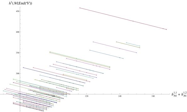
(b) Hypersurface models part 2

Figure 1: Plot of the topological data of hypersurfaces in toric varieties and their codimension two duals with full agreement. Each line corresponds to one class of dual models. Different colored overlapping lines correspond to different classes.

Different classes	Possibly smooth models	Classes without duals	Models with matching spectrum	Models with full agreement	Computed (different) line bundle cohom.
1,085	4,507	42	4,144 (100%)	1509 (94.6%)	(1,481,539) 3,069,067

Table 2: Some data on the landscape study: Starting point are hypersurfaces in toric varieties that are given by the polytopes with at most 9 lattice points. The percent numbers in the parentheses in column 4 and 5 only cover models where these numbers could actually be calculated. In column 5, by “full agreement” we mean that the chiral spectrum of dual models as well as the sum of complex structure, Kähler and bundle deformations agree.

4.3 CICY of two hypersurfaces

As a second scan we took a list of codimension 2 complete intersections in weighted projective spaces as a start, rather than just single hypersurfaces. This list can be found online at [34]. For our scan we simply ran through the first $2,780$ ambient spaces and chose the $16,029$ possible nef partitions as starting points. All these nef partitions correspond to topologically distinct Calabi-Yau manifolds that are complete intersections of two hypersurfaces in the corresponding weighted projective space. All dual models are codimension three complete intersections in toric varieties. In figures 2 and 3 we have displayed all the models where a full agreement of deformations and chiral spectrum was found. In table 3 we provide the summary of some details on the full scan.

Different classes	Possibly smooth models	Classes without duals	Models with matching spectrum	Models with full agreement	Computed (different) line bundle cohom.
16,961	79,204	718	64,332 (85 %)	20,336 (91%)	(38,807,002) 109,228,732

Table 3: Some data on landscape study. Starting point are codimension two complete intersections in weighted projective spaces.

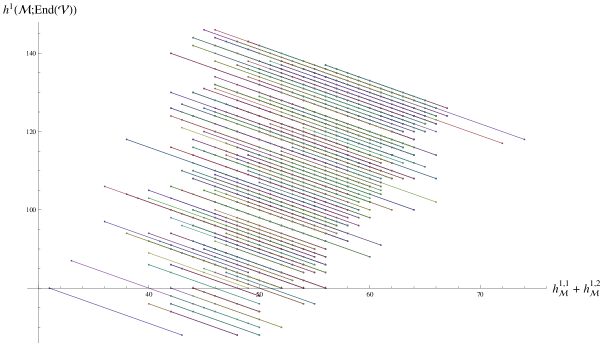
(a) Complete intersection models part 1

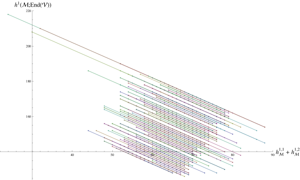
(b) Complete intersection models part 2

Figure 2: Plot of the topological data of codimension two complete intersections in weighted projective spaces and their codimension three duals. Each line corresponds to one class of dual models. Different colored overlapping lines correspond to different classes.

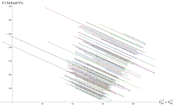
(a) Complete intersection models part 3

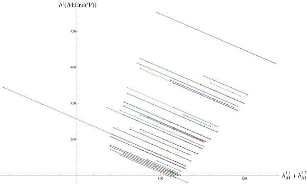
(b) Complete intersection models part 4

Figure 3: Plot of the topological data of codimension two complete intersections in weighted projective spaces and their codimension three duals. Each line corresponds to one class of dual models. Different colored overlapping lines correspond to different classes.

4.4 The mismatch

While we were performing the scan over the landscape, we found that the duality holds in most the cases, but not in all of them. In two different ways it actually happened to fail i.e. either such that the chiral spectrum did not match or that that the sum of total deformations of the Calabi-Yau and the bundle did not match. The chiral spectrum can fail to match for the following reasons:

• The Calabi-Yau manifold is not smooth and still contains singularities. In addition, the monad might not define a smooth vector bundle, but for instance merely a coherent sheaf with non-constant rank (see e.g. [18, 8] for a correct treatment of such configurations).

• During the scan we did not explicitly check whether the model we started with actually admits a phase that allows for the redefinition of the corresponding fields. So it might happen that such a phase did not exist which would forbid the exchange of specific $F$’s and $G$’s.

The mismatch of ${\rm D}({\cal M},{\cal V})\neq{\rm D}(\widetilde{\cal M},\widetilde{\cal V})$ can of course be traced back to the same reasons, but could also be happening since we assumed the bundle to be stable and furthermore the map $\varphi$ in (15) to be surjective.

Example:

Let us present a simple example where a mismatch occurs. Consider the following configuration with standard embedding:

$$\begin{array}[]{|c||c|}\hline\cr x_{i}&\Gamma^{j}\\ \hrule height=1.0pt\cr\begin{array}[]{cccccccc}-1&0&0&1&1&1\\ 1&1&1&0&0&0\end{array}&\begin{array}[]{ccc}-2\\ -3\end{array}\\ \hline\cr\end{array}\,.$$

One possible dual model of this configuration can be be obtained as

$$\begin{array}[]{|c||c|}\hline\cr x_{i}&\Gamma^{j}\\ \hrule height=1.0pt\cr\begin{array}[]{cccccccccc}0&0&0&0&0&0&1&1\\ -1&0&0&1&1&1&0&0\\ 1&1&1&0&0&0&3&0\end{array}&\begin{array}[]{cccc}-1&-1\\ -1&-1\\ -3&-3\end{array}\\ \hline\cr\end{array} \begin{array}[]{|c||c|}\hline\cr\Lambda^{a}&p_{l}\\ \hrule height=1.0pt\cr\begin{array}[]{cccccccc}0&0&0&1&0&0\\ -1&0&0&0&2&1\\ 1&1&1&0&0&0\end{array}&\begin{array}[]{ccc}-1\\ -2\\ -3\end{array}\\ \hline\cr\end{array}\,.$$

For the initial model $({\cal M},{\cal V})$ we calculate the following data

$$h_{S}^{\bullet}(V) = (0,86,2,0)\,,$$

$$h_{S}^{1,1}+h_{S}^{2,1}+h_{S}^{1}(\text{End}(V)) = 2+86+184=272\,,$$

whereas for the dual model we find

$$h_{\tilde{S}}^{\bullet}(\tilde{V}) = (0,86,2,0)\,,$$

$$h_{\tilde{S}}^{1,1}+h_{\tilde{S}}^{2,1}+h_{\tilde{S}}^{1}(\text{End}(\tilde{V})) = 3+78+195=276\,,$$

We observe that there is a mismatch of 4 for ${\rm D}({\cal M},{\cal V})$, but at the present state it is hard to determine the precise origin of this mismatch.

5 Conclusions

In this paper we have proposed a method to construct from almost any given $(0,2)$ heterotic model, dual models that generically have the same massless spectra. This procedure should work basically with all possible structure groups $SU(3),~{}SU(4),~{}SU(5)$ for the bundle and preserves all anomaly cancellation conditions. For the special case that Fermi superfields become uncharged in the dual model, it was suggested that an additional blowup of a $\mathbb{P}^{1}$ has to be performed. Furthermore it was pointed out that in these cases the duality transformation of the base could be understood as the resolution of a conifold singularity.

To provide evidence for our proposal, a large number of examples were investigated where the initial models were hypersurfaces in toric varieties and codimension two complete intersections in weighted projective spaces. For both types the initial configuration was the Calabi-Yau manifold equipped with a deformation of its tangent bundle of $SU(3)$ structure group. A great number of models agreed in all instances and an interpretation of the mismatch of the bundle deformations and an explanation of the mismatch of the chiral spectrum was suggested. There are a couple of things that would be interesting to investigate further:

Since it was not checked explicitly whether the bundle of a dual configuration is indeed a stable, it would be very useful to find a way or a requirement for the proposed procedure that ensures stability of the dual bundle.

We argued that deformations of the complex structure and of the bundle, that come from global section of line bundles on the Calabi-Yau manifold, are unobstructed. A mathematically rigorous treatment of these obstructions was recently presented in [24] and it would be interesting whether potential target space dual models also have the same number of unobstructed deformations.

The landscape study we performed, on the one hand, was quite extensive but, on the other hand, restricted to a particular class of models, namely those that arise from standard embeddings and hence have $SU(3)$ structure group. Even though for vector bundles with other structure groups the duality was checked in some cases, it would be interesting to see, if this works also for a much larger sample of models. In this respect, further checks would be possible, i.e. a matching of zero modes that live in $h^{1}_{\cal M}(\Lambda^{2}{\cal V})$ and $h^{1}({\cal M},\Lambda^{2}{\cal V}^{\ast})$.

Since such a large number of 83,711 models was analyzed, we are confident that a fair ratio really defines ”healthy” configurations. Nevertheless, since only consistency checks were made in order to detect singularities of the generated spaces, a closer analysis of the specific configuration would be necessary in order to ensure that the base as well as the bundle are indeed smooth. Since from the list of different Hodge numbers that were generated, there were quite some that turned out to be actually not yet discovered combinations of $(h^{2,1},h^{1,1})$, the explicit analysis of these spaces is a worthwhile thing to do [39].

For elliptically fibered Calabi-Yau threefolds with vector bundles defined via the spectral cover construction, it is known that there exist a higher dimensional framework, namely F-theory on Calabi-Yau fourfolds, in which the complex structure and bundle deformations are unified. In fact, considering a Calabi-Yau fourfould admitting two different K3-fibrations would also imply a duality between two seemingly different heterotic $(0,2)$ models. In this respect, it is an interesting question whether also in the present case of $(0,2)$ GLSMs a unified description exists, where the duality is manifest.

Acknowledgment

We would like to thank Benjamin Jurke for useful discussions and also for providing us with his Toric Triangulizer and related Mathematica scripts. We are also grateful for comments and discussions with Lara Anderson, Volker Braun, James Gray, Stefan Groot Nibbelink, Ilarion Melnikov and Bernhard Wurm. We would also like to thank the Erwin Schrödinger International Institute for Mathematical Physics (ESI) for hospitality.

Appendix A Anomaly cancellation

In this appendix, we show that the dual configuration $(\widetilde{\cal M},\widetilde{\cal V})$ satisfy the anomaly cancellation conditions (2), if they were satisfied by the initial one $({\cal M},{\cal V})$. For this purpose, let us start with a general configuration

$$V_{N_{1},...,N_{\delta}}[M_{1},...,M_{\gamma}]\longrightarrow\mathbb{P}_{Q_{1},...,Q_{d}}[S_{1},...,S_{c}]\,.$$

that satisfies the combinatorial relations (2):

$$\sum_{a=1}^{\delta}N_{a}^{(\alpha)}=\sum_{l=1}^{\gamma}M_{l}^{(\alpha)},\qquad\quad\sum_{i=1}^{d}Q_{i}^{(\alpha)}=\sum_{j=1}^{c}S_{j}^{(\alpha)}$$

$$\sum_{l=1}^{\gamma}M_{l}^{(\alpha)}M_{l}^{(\beta)}-\sum_{a=1}^{\delta}N_{a}^{(\alpha)}N_{a}^{(\beta)}=\sum_{j=1}^{c}S_{j}^{(\alpha)}S_{j}^{(\beta)}-\sum_{i=1}^{d}Q_{i}^{(\alpha)}Q_{i}^{(\beta)}\;,$$

for all $\alpha,\beta=1,\ldots,r$. We want to to show that this implies that the dual configuration,

$$V_{\tilde{N}_{1},\tilde{N}_{2},N_{3},...,N_{\delta}}[M_{1},M_{2},...,M_{\gamma}]\longrightarrow\mathbb{P}_{Q_{1},...,Q_{d},B}[\tilde{S}_{1},S_{3},...,S_{c},\tilde{B}]\,,$$

with charges given in table 3.2, still satisfies these relations. The new fields that changed comparing to the initial model read

$$\begin{split}\begin{array}[]{|c|c|c|c|c|c|c|c|c|}\hline\cr y_{1}&y_{2}&\tilde{\Gamma}^{1}&\tilde{\Gamma}^{B}&\tilde{F}_{1}{}^{1}&\tilde{F}_{2}{}^{1}&\tilde{\Lambda}^{1}&\tilde{\Lambda}^{2}&p_{1}\\ \hrule height=1.0pt\cr 1&1&-1&-1&0&1&1&0&-1\\ \hline\cr B&0&-(M_{1}-N_{1})&-(M_{1}-N_{2})&S_{1}&B&M_{1}-S_{1}&M_{1}-B&-M_{1}\\ \hline\cr\end{array}\;.\end{split}$$

Since $y_{1}$ was chosen in a way that

$$\begin{split}B+S_{1}=||F_{1}{}^{1}||+||F_{2}{}^{1}||=2M_{1}-N_{1}-N_{2}\end{split}$$ (84)

we get

$$\begin{split}||\tilde{F}_{2}{}^{1}||&=\left(\!\begin{array}[]{c}1\\ 2M_{1}-N_{1}-N_{2}-S_{1}\end{array}\!\right)\,,\\ ||\tilde{\Lambda}^{2}||&=\left(\!\begin{array}[]{c}1\\ -M_{1}+N_{1}+N_{2}+S_{1}\end{array}\!\right)\;.\end{split}$$ (85)

Linear relations:

Let us refer to the $U(1)$ charges that belong to the blown up $\mathbb{P}^{1}$ as new $U(1)$ charges. The Calabi-Yau condition, i.e. the second equation in (2) for the dual model is clear for the new $U(1)$ charges. For the other $U(1)$’s it reads

$$\sum_{i=1}^{d}Q_{i}^{(\alpha)}+B^{(\alpha)} = {\sum_{j=2}^{c}S_{j}^{(\alpha)}}+(M_{1}^{(\alpha)}-N_{1}^{(\alpha)})$$

$$\phantom{aaaaaaaaaa}+(M_{1}^{(\alpha)}-N_{2}^{(\alpha)})$$

$$\Leftrightarrow\ \sum_{i=1}^{d}Q_{i}^{(\alpha)}+2M_{1}^{(\alpha)}-N_{1}^{(\alpha)}-N_{2}^{(\alpha)}-S_{1}^{(\alpha)} = \sum_{j=2}^{c}S_{j}^{(\alpha)}+2M_{1}^{(\alpha)}-N_{1}^{(\alpha)}-N_{2}^{(\alpha)}$$

$$\Leftrightarrow\ {\sum_{i=1}^{d}Q_{i}^{(\alpha)}}+2M_{1}^{(\alpha)}-N_{1}^{(\alpha)}-N_{2}^{(\alpha)} = {\sum_{j=1}^{c}S_{j}^{(\alpha)}}+2M_{1}^{(\alpha)}-N_{1}^{(\alpha)}-N_{2}^{(\alpha)}$$

$$\Leftrightarrow\ {\sum_{i=1}^{d}Q_{i}^{(\alpha)}} = {\sum_{j=1}^{c}S_{j}^{(\alpha)}}\qquad{\square}$$

The second linear relation is also satisfied:

$$\sum_{a=3}^{\delta}N_{a}^{(\alpha)}+(M_{1}-S_{1})+(-M_{1}+N_{1}+N_{2}+S_{1}) = \sum_{l=1}^{\gamma}M_{l}^{(\alpha)}$$

$$\sum_{a=1}^{\delta}N_{a}^{(\alpha)} = \sum_{l=1}^{\gamma}M_{l}^{(\alpha)}\qquad{\square}$$

Quadratic relations:

Now lets have a look at the quadratic relations in (2). There are three different cases. The first where only the new $U(1)$ charges are involved, the second where old and new charges get mixed and the third where only the old charges are considered. Lets start with the first, which is obvious since only few changes were made:

$$1^{2}+1^{2}-((-1)^{2}+(-1)^{2})=1^{2}-(-1)^{2}\qquad\Leftrightarrow\qquad 0=0\qquad{\square}$$

For the second one we find:

$$(M_{1}-N_{1})+(M_{1}-N_{2})-(B-0) = M_{1}-((M_{1}-S_{1})+0)$$

$$\Leftrightarrow\ 2M_{1}-B = N_{1}+N_{2}+S_{1}$$

$$\Leftrightarrow\ 2M_{1}-2M_{1}+N_{1}+N_{2}+S_{1} = N_{1}+N_{2}+S_{1}$$

$$\Leftrightarrow\ N_{1}+N_{2}+S_{1} = N_{1}+N_{2}+S_{1}\qquad{\square}$$

The last only involves the old $U(1)$ charges:

$$\sum_{l=1}^{\gamma}M_{l}^{(\alpha)}M_{l}^{(\beta)}-\sum_{a=3}^{\delta}N_{a}^{(\alpha)}N_{a}^{(\beta)}-\tilde{N}_{1}^{(\alpha)}\tilde{N}_{1}^{(\beta)}-\tilde{N}_{2}^{(\alpha)}\tilde{N}_{2}^{(\beta)}$$

$$=\sum_{j=2}^{c}S_{j}^{(\alpha)}S_{j}^{(\beta)}+\tilde{S}_{1}^{(\alpha)}\tilde{S}_{1}^{(\beta)}+\tilde{S}_{2}^{(\alpha)}\tilde{S}_{2}^{(\beta)}-\sum_{i=1}^{d}Q_{i}^{(\alpha)}Q_{i}^{(\beta)}-B^{(\alpha)}B^{(\beta)}-0$$

$$\Leftrightarrow \sum_{a=1}^{2}N_{a}^{(\alpha)}N_{a}^{(\beta)}-\tilde{N}_{1}^{(\alpha)}\tilde{N}_{1}^{(\beta)}-\tilde{N}_{2}^{(\alpha)}\tilde{N}_{2}^{(\beta)}$$

$$=-S_{1}^{(\alpha)}S_{1}^{(\beta)}+\tilde{S}_{1}^{(\alpha)}\tilde{S}_{1}^{(\beta)}+\tilde{S}_{2}^{(\alpha)}\tilde{S}_{2}^{(\beta)}-B^{(\alpha)}B^{(\beta)}$$

$$\Leftrightarrow \sum_{a=1}^{2}N_{a}^{(\alpha)}N_{a}^{(\beta)}-(M_{1}^{(\alpha)}-S_{1}^{(\alpha)})(M_{1}^{(\beta)}-S_{1}^{(\beta)})-(M_{1}^{(\alpha)}-B^{(\alpha)})(M_{1}^{(\beta)}-B^{(\beta)})$$

$$=-S_{1}^{(\alpha)}S_{1}^{(\beta)}+(M_{1}^{(\alpha)}-N_{1}^{(\alpha)})(M_{1}^{(\beta)}-N_{1}^{(\beta)})$$

$$\phantom{aaaaaaaaaa}+(M_{1}^{(\alpha)}-N_{2}^{(\alpha)})(M_{1}^{(\beta)}-N_{2}^{(\beta)})-B^{(\alpha)}B^{(\beta)}\,,$$

where we used the initial quadratic relations from (2) in the first step. As an intermediate step, lets evaluate the third and fourth term of the right hand side of

$$\begin{split}-(M_{1}^{(\alpha)}-B^{(\alpha)})(M_{1}^{(\beta)}-&B^{(\beta)})=\\ &-M_{1}^{(\alpha)}M_{1}^{(\beta)}-B^{(\alpha)}B^{(\beta)}+M_{1}^{(\alpha)}B^{(\beta)}+B^{(\alpha)}M_{1}^{(\beta)}\end{split}$$ (87)

which reads

$$M_{1}^{(\alpha)}B^{(\beta)} = 2M_{1}^{(\alpha)}M_{1}^{(\beta)}-M_{1}^{(\alpha)}N_{1}^{(\beta)}-M_{1}^{(\alpha)}N_{2}^{(\beta)}-M_{1}^{(\alpha)}S_{1}^{(\beta)}\,,$$

$$M_{1}^{(\beta)}B^{(\alpha)} = 2M_{1}^{(\beta)}M_{1}^{(\alpha)}-M_{1}^{(\beta)}N_{1}^{(\alpha)}-M_{1}^{(\beta)}N_{2}^{(\alpha)}-M_{1}^{(\beta)}S_{1}^{(\alpha)}$$

and hence it folllows

$$\begin{split}M_{1}^{(\alpha)}B^{(\beta)}+M_{1}^{(\beta)}B^{(\alpha)}=&M_{1}^{(\alpha)}M_{1}^{(\beta)}\\ &+(M_{1}^{(\alpha)}-N_{1}^{(\alpha)})(M_{1}^{(\beta)}-N_{1}^{(\beta)})-N_{1}^{(\alpha)}N_{1}^{(\beta)}\\ &+(M_{1}^{(\alpha)}-N_{2}^{(\alpha)})(M_{1}^{(\beta)}-N_{2}^{(\beta)})-N_{2}^{(\alpha)}N_{2}^{(\beta)}\\ &+(M_{1}^{(\alpha)}-S_{1}^{(\alpha)})(M_{1}^{(\beta)}-S_{1}^{(\beta)})-S_{1}^{(\alpha)}S_{1}^{(\beta)}\,.\end{split}$$ (88)

Pluggin (88) back into (87) and (87) back into (A), we get

$$\sum_{a=1}^{2}N_{a}^{(\alpha)}N_{a}^{(\beta)}-(M_{1}^{(\alpha)}-S_{1}^{(\alpha)})(M_{1}^{(\beta)}-S_{1}^{(\beta)})+M_{1}^{(\alpha)}M_{1}^{(\beta)}-M_{1}^{(\alpha)}M_{1}^{(\beta)}$$

$$-B^{(\alpha)}B^{(\beta)}+(M_{1}^{(\alpha)}-N_{1}^{(\alpha)})(M_{1}^{(\beta)}-N_{1}^{(\beta)})-N_{1}^{(\alpha)}N_{1}^{(\beta)}$$

$$+(M_{1}^{(\alpha)}-N_{2}^{(\alpha)})(M_{1}^{(\beta)}-N_{2}^{(\beta)})-N_{2}^{(\alpha)}N_{2}^{(\beta)}$$

$$+(M_{1}^{(\alpha)}-S_{1}^{(\alpha)})(M_{1}^{(\beta)}-S_{1}^{(\beta)})-S_{1}^{(\alpha)}S_{1}^{(\beta)}$$

$$= -S_{1}^{(\alpha)}S_{1}^{(\beta)}+(M_{1}^{(\alpha)}-N_{1}^{(\alpha)})(M_{1}^{(\beta)}-N_{1}^{(\beta)})$$

$$+(M_{1}^{(\alpha)}-N_{2}^{(\alpha)})(M_{1}^{(\beta)}-N_{2}^{(\beta)})-B^{(\alpha)}B^{(\beta)}\,,$$

$$\Leftrightarrow 0=0\qquad{\square}\,.$$

Since we did not assume that $M_{1}=S_{1}$, the whole calculation is valid for both cases described in 3.2. In fact, it can be shown that one can exchange an arbitrary number of $G$’s with $F$’s, as long as at most one uncharged Fermi superfield appears.