Infrared behavior of interacting bosons at zero temperature

Abstract

We review the infrared behavior of interacting bosons at zero temperature. After a brief discussion of the Bogoliubov approximation and the breakdown of perturbation theory due to infrared divergences, we present two approaches that are free of infrared divergences – Popov’s hydrodynamic theory and the non-perturbative renormalization group – and allow us to obtain the exact infrared behavior of the correlation functions. We also point out the connection between the infrared behavior in the superfluid phase and the critical behavior at the superfluid–Mott-insulator transition in the Bose-Hubbard model.

I Introduction

Many of the predictions of the Bogoliubov theory of superfluidity Bogoliubov (1947) have been confirmed experimentally, in particular in ultracold atomic gases Dalfovo et al. (1999); Leggett (2001). Nevertheless a clear understanding of the infrared behavior of interacting bosons at zero temperature has remained a challenging theoretical issue for a long time. Early attempts to go beyond the Bogoliubov theory have revealed a singular perturbation theory plagued by infrared divergences due to the presence of the Bose-Einstein condensate and the Goldstone mode Hugenholtz and Pines (1959); Gavoret and Nozières (1964); Beliaev (1958a, b). In the 1970s, Nepomnyashchii and Nepomnyashchii proved that the anomalous self-energy vanishes at zero frequency and momentum in dimension $d\leq 3$ Nepomnyashchii and Nepomnyashchii (1975). This exact result shows that the Bogoliubov approximation, where the linear spectrum and the superfluidity rely on a finite value of the anomalous self-energy, breaks down at low energy. As realized latter on Nepomnyashchii and Nepomnyashchii (1978); Nepomnyashchii (1983), the singular perturbation theory is a direct consequence of the coupling between transverse and longitudinal fluctuations and reflects the divergence of the longitudinal susceptibility – a general phenomenon in systems with a continuous broken symmetry Patasinskij and Pokrovskij (1973).

In this paper, we review the infrared behavior of interacting bosons. A more detailed discussion together with a comparison to the classical O($N$) model can be found in Ref. Dupuis10 . In Sec. II, we briefly review the Bogoliubov theory and the appearance of infrared divergences in perturbation theory. We introduce the Ginzburg momentum scale $p_{G}$ signaling the breakdown of the Bogoliubov approximation. In Sec. III, we discuss Popov’s hydrodynamic approach based on a phase-density representation of the boson field Popov (1972); Popov and Seredniakov (1979); Popov (1983). This approach allows one to derive the order parameter correlation function without encountering infrared divergences. The non-perturbative renormalization group (NPRG) provides another approach free of infrared divergences which yields the exact infrared behavior of the normal and anomalous single-particle propagators (Sec. IV) Castellani et al. (1997); Pistolesi et al. (2004); Wetterich (2008); Floerchinger and Wetterich (2008); Dupuis and Sengupta (2007); Dupuis (2009a, b); Sinner et al. (2009); Sinner10 . In the last section, we discuss the critical behavior at the superfluid–Mott-insulator transition in the Bose-Hubbard model and its connection to the infrared behavior in the superfluid phase.

II Perturbation theory and breakdown of the Bogoliubov approximation

We consider interacting bosons at zero temperature with the (Euclidean) action

$$S=\int dx\left[\psi^{*}\left({\partial_{\tau}}-\mu-\frac{\boldsymbol{\nabla}^{2}}{2m}\right)\psi+\frac{g}{2}(\psi^{*}\psi)^{2}\right],$$ (1)

where $\psi(x)$ is a bosonic (complex) field, $x=({\bf r},\tau)$, and $\int dx=\int_{0}^{\beta}d\tau\int d^{d}r$. $\tau\in[0,\beta]$ is an imaginary time, $\beta\to\infty$ the inverse temperature, and $\mu$ denotes the chemical potential. The interaction is assumed to be local in space and the model is regularized by a momentum cutoff $\Lambda$. We consider a space dimension $d>1$.

Introducing the two-component field

$$\Psi(p)=\left(\begin{array}[]{c}\psi(p)\\ \psi^{*}(-p)\end{array}\right),\quad\Psi^{\dagger}(p)=\bigl{(}\psi^{*}(p),\psi(-p)\bigr{)}$$ (2)

(with $p=({\bf p},i\omega)$ and $\omega$ a Matsubara frequency), the one-particle (connected) propagator becomes a $2\times 2$ matrix whose inverse in Fourier space is given by

$$\left(\begin{array}[]{cc}i\omega+\mu-\epsilon_{\bf p}-\Sigma_{\rm n}(p)&-\Sigma_{\rm an}(p)\\ -\Sigma_{\rm an}^{*}(p)&-i\omega+\mu-\epsilon_{\bf p}-\Sigma_{\rm n}(-p)\end{array}\right),$$ (3)

where $\Sigma_{\rm n}$ and $\Sigma_{\rm an}$ are the normal and anomalous self-energies, respectively, and $\epsilon_{\bf p}={\bf p}^{2}/2m$. If we choose the order parameter $\langle\psi(x)\rangle=\sqrt{n_{0}}$ to be real (with $n_{0}$ the condensate density), then the anomalous self-energy $\Sigma_{\rm an}(p)$ is real.

II.1 Bogoliubov approximation

The Bogoliubov approximation is a Gaussian fluctuation theory about the saddle point solution $\psi(x)=\sqrt{n_{0}}=\sqrt{\mu/g}$. It is equivalent to a zero-loop calculation of the self-energies Abrikosov et al. (1975); Fetter and Walecka (2003),

$$\Sigma_{\rm n}^{(0)}(p)=2gn_{0},\quad\Sigma_{\rm an}^{(0)}(p)=gn_{0}.$$ (4)

This yields the (connected) propagators

$$\begin{split}G_{\rm n}^{(0)}(p)&=-\langle\psi(p)\psi^{*}(p)\rangle_{c}=\frac{-i\omega-\epsilon_{\bf p}-gn_{0}}{\omega^{2}+E_{\bf p}^{2}},\\ G_{\rm an}^{(0)}(p)&=-\langle\psi(p)\psi(-p)\rangle_{c}=\frac{gn_{0}}{\omega^{2}+E_{\bf p}^{2}},\end{split}$$ (5)

where $E_{\bf p}=[\epsilon_{\bf p}(\epsilon_{\bf p}+2gn_{0})]^{1/2}$ is the Bogoliubov quasi-particle excitation energy. When $|{\bf p}|$ is larger than the healing momentum $p_{c}=(2gmn_{0})^{1/2}$, the spectrum $E_{\bf p}\simeq\epsilon_{\bf p}+gn_{0}$ is particle-like, whereas it becomes sound-like for $|{\bf p}|\ll p_{c}$ with a velocity $c=\sqrt{gn_{0}/m}$. In the weak-coupling limit, $n_{0}\simeq\bar{n}$ ($\bar{n}$ is the mean boson density) and $p_{c}$ can equivalently be defined as $p_{c}=(2gm\bar{n})^{1/2}$.

It is convenient to write the boson field

$$\psi(x)=\frac{1}{\sqrt{2}}[\psi_{1}(x)+i\psi_{2}(x)]$$ (6)

in terms of two real fields $\psi_{1}$ and $\psi_{2}$, which allows us to distinguish between longitudinal ($\psi_{1}$) and transverse ($\psi_{2}$) fluctuations. In the hydrodynamic regime $|{\bf p}|\ll p_{c}$,

$$\begin{split}G_{11}^{(0)}(p)&=\frac{\epsilon_{\bf p}}{\omega^{2}+c^{2}{\bf p}^{2}},\\ G_{22}^{(0)}(p)&=\frac{2gn_{0}}{\omega^{2}+c^{2}{\bf p}^{2}},\\ G_{12}^{(0)}(p)&=-\frac{\omega}{\omega^{2}+c^{2}{\bf p}^{2}},\end{split}$$ (7)

where $G_{ij}({\bf p})=\langle\psi_{i}({\bf p})\psi_{j}(-{\bf p})\rangle_{c}$. In the Bogoliubov approximation, the occurrence of a linear spectrum at low energy (which implies superfluidity according to Landau’s criterion) is due to $\Sigma_{\rm an}(p=0)$ being nonzero.

II.2 Infrared divergences and the Ginzburg scale

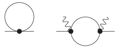
Figure 1: One-loop correction $\Sigma^{(1)}$ to the self-energy. The dots represent the bare interaction, the zigzag lines the order parameter $\sqrt{n_{0}}$, and the solid lines the connected propagator $G^{(0)}$.

Let us now consider the lowest-order (one-loop) correction $\Sigma^{(1)}$ to the Bogoliubov result $\Sigma^{(0)}$. For $d\leq 3$, the second diagram of Fig. 1 gives a divergent contribution when the two internal lines correspond to transverse fluctuations, which indicates a breakdown of perturbation theory and therefore the Bogoliubov approximation. Retaining only the divergent part, we obtain

$$\Sigma_{\rm n}^{(1)}(p)\simeq\Sigma_{\rm an}^{(1)}(p)\simeq-\frac{1}{2}g^{2}n_{0}\int_{q}G_{22}^{(0)}(q)G_{22}^{(0)}(p+q),$$ (8)

where we use the notation $\int_{q}=\int_{-\infty}^{\infty}\frac{d\omega^{\prime}}{2\pi}\int_{\bf q}$. For small $p$, the main contribution to the $q$ integral in (8) comes from momenta $|{\bf q}|\lesssim p_{c}$ and frequencies $|\omega^{\prime}|\lesssim cp_{c}$. We can then use (7) and obtain

$$\Sigma_{\rm n}^{(1)}(p)\simeq\Sigma_{\rm an}^{(1)}(p)\simeq-2\frac{g^{4}n_{0}^{3}}{c^{3}}A_{d+1}\left({\bf p}^{2}+\frac{\omega^{2}}{c^{2}}\right)^{(d-3)/2}$$ (9)

if $d<3$ and

$$\Sigma_{\rm n}^{(1)}(p)\simeq\Sigma_{\rm an}^{(1)}(p)\simeq-\frac{g^{4}n_{0}^{3}}{c^{3}}A_{4}\ln\left(\frac{p^{2}_{c}}{{\bf p}^{2}+\omega^{2}/c^{2}}\right)$$ (10)

if $d=3$, where

$$A_{d}=\left\{\begin{array}[]{lcc}-\frac{2^{1-d}\pi^{1-d/2}}{\sin(\pi d/2)}\frac{\Gamma(d/2)}{\Gamma(d-1)}&\mbox{if}&d<4,\\ \frac{1}{8\pi^{2}}&\mbox{if}&d=4.\end{array}\right.$$ (11)

We can estimate the characteristic (Ginzburg) momentum scale $p_{G}$ below which the Bogoliubov approximation breaks down from the condition $|\Sigma_{\rm n}^{(1)}(p)|\sim\Sigma_{\rm n}^{(0)}(p)$ or $|\Sigma_{\rm an}^{(1)}(p)|\sim\Sigma_{\rm an}^{(0)}(p)$ for $|{\bf p}|=p_{G}$ and $|\omega|=cp_{G}$,

$$p_{G}\sim\left\{\begin{array}[]{lcc}(A_{d+1}gmp_{c})^{1/(3-d)}&\mbox{if}&d<3,\\ p_{c}\exp\left(-\frac{1}{A_{4}gmp_{c}}\right)&\mbox{if}&d=3.\end{array}\right.$$ (12)

This result can be rewritten as

$$p_{G}\sim\left\{\begin{array}[]{lcc}p_{c}(A_{d+1}\tilde{g}^{d/2})^{1/(3-d)}&\mbox{if}&d<3,\\ p_{c}\exp\left(-\frac{1}{A_{4}\sqrt{2}\tilde{g}^{3/2}}\right)&\mbox{if}&d=3,\end{array}\right.$$ (13)

where

$$\tilde{g}=gm\bar{n}^{1-2/d}\sim\left(\frac{p_{c}}{\bar{n}^{1/d}}\right)^{2}$$ (14)

is the dimensionless coupling constant obtained by comparing the mean interaction energy per particle $g\bar{n}$ to the typical kinetic energy $1/m\bar{r}^{2}$ where $\bar{r}\sim\bar{n}^{-1/d}$ is the mean distance between particles Petrov et al. (2004). A superfluid is weakly correlated if $\tilde{g}\ll 1$, i.e. $p_{G}\ll p_{c}\ll\bar{n}^{1/d}$ (the characteristic momentum scale $\bar{n}^{1/d}$ does however not play any role in the weak-coupling limit) Capogrosso-Sansone et al. (2010). In this case, the Bogoliubov theory applies to a large part of the spectrum where the dispersion is linear (i.e. $|{\bf p}|\lesssim p_{c}$) and breaks down only at very small momenta $|{\bf p}|\lesssim p_{G}\ll p_{c}$. When the dimensionless coupling $\tilde{g}$ becomes of order unity, the three characteristic momentum scales $p_{G}\sim p_{c}\sim\bar{n}^{1/d}$ become of the same order. The momentum range $[p_{G},p_{c}]$ where the linear spectrum can be described by the Bogoliubov theory is then suppressed. We expect the strong-coupling regime $\tilde{g}\gg 1$ to be governed by a single characteristic momentum scale, namely $\bar{n}^{1/d}$.

II.3 Vanishing of the anomalous self-energy

The exact values of $\Sigma_{\rm n}(p=0)$ and $\Sigma_{\rm an}(p=0)$ can be obtained using the U(1) symmetry of the action, i.e. the invariance under the field transformation $\psi(x)\to e^{i\theta}\psi(x)$ and $\psi^{*}(x)\to e^{-i\theta}\psi^{*}(x)$. On the one hand, the self-energies satisfy the Hugenholtz-Pines theorem Hugenholtz and Pines (1959),

$$\Sigma_{\rm n}(p=0)-\Sigma_{\rm an}(p=0)=\mu.$$ (15)

On the other hand, the anomalous self-energy vanishes,

$$\Sigma_{\rm an}(p=0)=0.$$ (16)

The last result was first proven by Nepomnyashchii and Nepomnyashchii Nepomnyashchii and Nepomnyashchii (1975); Sinner10 ; Dupuis10 . It shows that the Bogoliubov theory, where the linear spectrum and the superfluidity rely on a finite value of the anomalous self-energy, breaks down at low energy in agreement with the conclusions drawn from perturbation theory (Sec. II.2).

III Popov’s hydrodynamic theory

It was realized by Popov that the phase-density representation of the boson field $\psi=\sqrt{n}e^{i\theta}$ leads to a theory free of infrared divergences Popov (1972, 1983). In this section, we show how this allows us to obtain the infrared behavior of the propagators $G_{\rm n}(p)$ and $G_{\rm an}(p)$ without encountering infrared divergences Popov and Seredniakov (1979).

III.1 Hydrodynamic action

In terms of the density and phase fields, the action reads

$$S[n,\theta]=\int dx\left[in\dot{\theta}+\frac{n}{2m}(\boldsymbol{\nabla}\theta)^{2}+\frac{(\boldsymbol{\nabla}n)^{2}}{8mn}-\mu n+\frac{g}{2}n^{2}\right].$$ (17)

At the saddle-point level, $n(x)=\bar{n}=\mu/g$. Expanding the action to second order in $\delta n=n-\bar{n}$, $\dot{\theta}$ and $\boldsymbol{\nabla}\theta$, we obtain

$$S[\delta n,\theta]=\int dx\left[i\delta n\dot{\theta}+\frac{\bar{n}}{2m}(\boldsymbol{\nabla}\theta)^{2}+\frac{(\boldsymbol{\nabla}n)^{2}}{8m\bar{n}}+\frac{g}{2}(\delta n)^{2}\right].$$ (18)

The higher-order terms can be taken into account within perturbation theory and only lead to finite corrections of the coefficients of the hydrodynamic action (18) Popov (1983).

We deduce the correlation functions of the hydrodynamic variables,

$$\begin{split}G_{nn}(p)&=\langle\delta n(p)\delta n(-p)\rangle=\frac{\bar{n}}{m}\frac{{\bf p}^{2}}{\omega^{2}+E_{\bf p}^{2}},\\ G_{n\theta}(p)&=\langle\delta n(p)\theta(-p)\rangle=-\frac{\omega}{\omega^{2}+E_{\bf p}^{2}},\\ G_{\theta\theta}(p)&=\langle\theta(p)\theta(-p)\rangle=\frac{\frac{{\bf p}^{2}}{4m\bar{n}}+g}{\omega^{2}+E_{\bf p}^{2}},\end{split}$$ (19)

where $E_{\bf p}$ is the Bogoliubov excitation energy defined in Sec. II.1. In the hydrodynamic regime $|{\bf p}|\ll p_{c}=\sqrt{2gm\bar{n}}$,

$$\begin{split}G_{nn}(p)&=\frac{\bar{n}}{m}\frac{{\bf p}^{2}}{\omega^{2}+c^{2}{\bf p}^{2}},\\ G_{n\theta}(p)&=-\frac{\omega}{\omega^{2}+c^{2}{\bf p}^{2}},\\ G_{\theta\theta}(p)&=\frac{mc^{2}}{\bar{n}}\frac{1}{\omega^{2}+c^{2}{\bf p}^{2}},\end{split}$$ (20)

where $c=\sqrt{g\bar{n}/m}$ is the Bogoliubov sound mode velocity. It can be shown that Eqs. (20) are exact in the hydrodynamic limit $|{\bf p}|,|\omega|/c\ll p_{c}$ provided that $c$ is the exact sound mode velocity and $\bar{n}$ the actual mean density (which may differ from $\mu/g$) Popov (1983); Dupuis10 .

III.2 Normal and anomalous propagators

To compute the propagator of the $\psi$ field, we write

$$\psi(x)=\sqrt{n_{0}+\delta n(x)}e^{i\theta(x)},$$ (21)

where $n_{0}=|\langle\psi(x)\rangle|^{2}=|\langle\sqrt{n(x)}e^{i\theta(x)}\rangle|^{2}$ is the condensate density. For a weakly-interacting superfluid, $n_{0}\simeq\bar{n}$, and we expect the fluctuations $\delta n$ to be small. Let us assume that the superfluid order parameter $\langle\psi(x)\rangle=\sqrt{n_{0}}$ is real. Transverse and longitudinal fluctuations are then expressed as

$$\begin{split}\delta\psi_{2}&=\sqrt{2n_{0}}\theta+\cdots\\ \delta\psi_{1}&=\frac{\delta n}{\sqrt{2n_{0}}}-\sqrt{\frac{n_{0}}{2}}\theta^{2}+\cdots\end{split}$$ (22)

where the ellipses stand for subleading contributions to the low-energy behavior of the correlation functions. For the transverse propagator, we obtain

$$G_{22}(p)\simeq 2n_{0}G_{\theta\theta}(p)=\frac{2n_{0}mc^{2}}{\bar{n}}\frac{1}{\omega^{2}+c^{2}{\bf p}^{2}}$$ (23)

to leading order in the hydrodynamic regime, while

$$G_{12}(p)\simeq G_{n\theta}(p)=-\frac{\omega}{\omega^{2}+c^{2}{\bf p}^{2}}.$$ (24)

The longitudinal propagator is given by

$$G_{11}(x) =\frac{1}{2n_{0}}G_{nn}(x)+\frac{n_{0}}{2}\langle\theta(x)^{2}\theta(0)^{2}\rangle_{c}$$

$$=\frac{1}{2n_{0}}G_{nn}(x)+n_{0}G_{\theta\theta}(x)^{2},$$ (25)

where the second line is obtained using Wick’s theorem. In Fourier space,

$$G_{11}(p)={} \frac{\bar{n}}{2mn_{0}}\frac{{\bf p}^{2}}{\omega^{2}+c^{2}{\bf p}^{2}}+n_{0}G_{\theta\theta}\star G_{\theta\theta}(p),$$ (26)

where

$$G_{\theta\theta}\star G_{\theta\theta}(p)=\int_{q}G_{\theta\theta}(q)G_{\theta\theta}(p+q).$$ (27)

The dominant contribution to the integral in (27) comes from momenta $|{\bf q}|\lesssim p_{c}$ and frequencies $|\omega^{\prime}|/c\lesssim p_{c}$, i.e.

$$G_{\theta\theta}\star G_{\theta\theta}(p)$$

$$=\left\{\begin{array}[]{lcc}A_{d+1}c\left(\frac{m}{\bar{n}}\right)^{2}\left({\bf p}^{2}+\frac{\omega^{2}}{c^{2}}\right)^{(d-3)/2}&\mbox{if}&d<3,\\ \frac{A_{4}}{2}c\left(\frac{m}{\bar{n}}\right)^{2}\ln\left(\frac{p_{c}^{2}}{{\bf p}^{2}+\frac{\omega^{2}}{c^{2}}}\right)&\mbox{if}&d=3.\end{array}\right.$$ (30)

By comparing the two terms in the rhs of (26) with $|{\bf p}|=p_{G}$ and $|\omega|=cp_{G}$, we recover the Ginzburg scale (12). For $|{\bf p}|,|\omega|/c\gg p_{G}$, the last term in the rhs of (26) can be neglected and we reproduce the result of the Bogoliubov theory (noting that $\bar{n}\simeq n_{0}$), while for $|{\bf p}|,|\omega|/c\ll p_{G}$, $G_{11}(p)\sim 1/(\omega^{2}+c^{2}{\bf p}^{2})^{(3-d)/2}$ is dominated by phase fluctuations (Goldstone regime). The longitudinal susceptibility $G_{11}({\bf p},i\omega=0)\sim 1/|{\bf p}|^{3-d}$ for ${\bf p}\to 0$ in contrast to the Bogoliubov approximation $G_{11}({\bf p},i\omega=0)=1/2mc^{2}$.

From these results, we deduce the hydrodynamic behavior of the normal propagator not (a),

$$G_{\rm n}(p)={} -\frac{1}{2}\left[G_{11}(p)-2iG_{12}(p)+G_{22}(p)\right]$$

$$={} -\frac{n_{0}mc^{2}}{\bar{n}}\frac{1}{\omega^{2}+c^{2}{\bf p}^{2}}$$

$$-\frac{i\omega}{\omega^{2}+c^{2}{\bf p}^{2}}-\frac{1}{2}G_{11}(p),$$ (31)

as well as that of the anomalous propagator,

$$G_{\rm an}(p)={} -\frac{1}{2}\left[G_{11}(p)-G_{22}(p)\right]$$

$$=\frac{n_{0}mc^{2}}{\bar{n}}\frac{1}{\omega^{2}+c^{2}{\bf p}^{2}}-\frac{1}{2}G_{11}(p),$$ (32)

where $G_{11}(p)$ is given by (26). The leading-order terms in (31) and (32) agree with the results of Gavoret and Nozières Gavoret and Nozières (1964) and are exact (see next section). The contribution of the diverging longitudinal correlation function was first identified by Nepomnyashchii and Nepomnyashchii Nepomnyashchii and Nepomnyashchii (1978) and later in Refs. Popov and Seredniakov (1979); Weichman (1988); Giorgini et al. (1992); Castellani et al. (1997); Pistolesi et al. (2004).

III.3 Normal and anomalous self-energies

To compute the self-energies $\Sigma_{\rm n}(p)$ and $\Sigma_{\rm an}(p)$, we use the relations

$$\begin{split}\Sigma_{\rm n}(p)&=G_{0}^{-1}(p)-\frac{G_{\rm n}(-p)}{G_{\rm n}(p)G_{\rm n}(-p)-G_{\rm an}(p)^{2}},\\ \Sigma_{\rm an}(p)&=\frac{G_{\rm an}(p)}{G_{\rm n}(p)G_{\rm n}(-p)-G_{\rm an}(p)^{2}}.\end{split}$$ (33)

This yields Popov and Seredniakov (1979); Dupuis10

$$\Sigma_{\rm an}(p) =\Sigma_{\rm n}(p)-G_{0}^{-1}(p)$$

$$=\left\{\begin{array}[]{lcc}\frac{\bar{n}^{2}}{2A_{d+1}c^{4-d}n_{0}m^{2}}(\omega^{2}+c^{2}{\bf p}^{2})^{(3-d)/2}&\mbox{if}&d<3,\\ \frac{\bar{n}^{2}}{A_{4}cn_{0}m^{2}}\left[\ln\left(\frac{\omega^{2}+c^{2}{\bf p}^{2}}{c^{2}p_{c}^{2}}\right)\right]^{-1}&\mbox{if}&d=3,\end{array}\right.$$ (36)

in the infrared limit $|{\bf p}|,|\omega|/c\ll p_{G}$, where $G_{0}^{-1}(p)=i\omega-\epsilon_{\bf p}+\mu$. Equations (36) agree with the exact results (15,16) and show that $\Sigma_{\rm n}(p)$ and $\Sigma_{\rm an}(p)$ are dominated by non-analytic terms for $p\to 0$. This non-analyticity reflects the singular behavior of the longitudinal correlation function

$$G_{11}(p)\simeq\frac{1}{2\Sigma_{\rm an}(p)}$$ (37)

in the low-energy limit.

IV The non-perturbative RG

The NPRG provides another way to circumvent the difficulties of perturbation theory and derive the correlation functions in the low-energy limit Castellani et al. (1997); Pistolesi et al. (2004); Dupuis and Sengupta (2007); Dupuis (2009a, b); Wetterich (2008); Floerchinger and Wetterich (2008); Sinner et al. (2009); Sinner10 . The strategy of the NPRG is to build a family of theories indexed by a momentum scale $k$ such that fluctuations are smoothly taken into account as $k$ is lowered from the microscopic scale $\Lambda$ down to 0 Berges et al. (2002); Delamotte . This is achieved by adding to the action (1) an infrared regulator term

$$\Delta S_{k}[\psi]=\frac{1}{2}\sum_{p,i}\psi_{i}(-p)R_{k}(p)\psi_{i}(p),$$ (38)

where $\psi_{1}$ and $\psi_{2}$ are the two real fields introduced in Sec. II.1 [Eq. (6)]. The main quantity of interest is the so-called average effective action

$$\Gamma_{k}[\phi]=-\ln Z_{k}[J]+\sum_{p,i}J_{i}(-p)\phi_{i}(p)-\Delta S_{k}[\phi],$$ (39)

defined as a modified Legendre transform of $-\ln Z_{k}[J]$ which includes the subtraction of $\Delta S_{k}[\phi]$. $J_{i}$ denotes an external source that couples linearly to the boson field $\psi_{i}$ and $\phi_{i}(x)=\langle\psi_{i}(x)\rangle$ is the superfluid order parameter. The cutoff function $R_{k}$ is chosen such that at the microscopic scale $\Lambda$ it suppresses all fluctuations, so that the mean-field approximation $\Gamma_{\Lambda}[\phi]=S[\phi]$ becomes exact. The effective action of the original model (1) is given by $\Gamma_{k=0}$ provided that $R_{k=0}$ vanishes. For a generic value of $k$, the cutoff function $R_{k}(p)$ suppresses fluctuations with momentum $|{\bf p}|\lesssim k$ and frequency $|\omega|\lesssim ck$ but leaves those with $|{\bf p}|,|\omega|/c\gtrsim k$ unaffected ($c\equiv c_{k}$ is the velocity of the Goldstone mode). The dependence of the average effective action on $k$ is given by Wetterich’s equation Wetterich (1993)

$$\partial_{t}\Gamma_{k}[\phi]=\frac{1}{2}{\rm Tr}\left\{\dot{R}_{k}\left(\Gamma^{(2)}_{k}[\phi]+R_{k}\right)^{-1}\right\},$$ (40)

where $t=\ln(k/\Lambda)$ and $\dot{R}_{k}=\partial_{t}R_{k}$. $\Gamma^{(2)}_{k}[\phi]$ denotes the second-order functional derivative of $\Gamma_{k}[\phi]$. In Fourier space, the trace involves a sum over momenta and frequencies as well as the internal index of the $\phi$ field. We choose the cutoff function Dupuis (2009b)

$$R_{k}(p)=\frac{Z_{A,k}}{2m}\left({\bf p}^{2}+\frac{\omega^{2}}{c_{0}^{2}}\right)r\left(\frac{{\bf p}^{2}}{k^{2}}+\frac{\omega^{2}}{k^{2}c_{0}^{2}}\right),$$ (41)

where $r(Y)=(e^{Y}-1)^{-1}$. The $k$-dependent variable $Z_{A,k}$ is defined below. A natural choice for the velocity $c_{0}$ would be the actual ($k$-dependent) velocity $c_{k}$ of the Goldstone mode. In the weak coupling limit, however, the Goldstone mode velocity renormalizes only weakly and is well approximated by the $k$-independent value $c_{0}=\sqrt{g\bar{n}/m}$.

IV.1 Derivative expansion and infrared behavior

Because of the regulator term $\Delta S_{k}$, the vertices $\Gamma^{(n)}_{k,i_{1}\cdots i_{n}}(p_{1},\cdots,p_{n})$ are smooth functions of momenta and frequencies and can be expanded in powers of ${\bf p}_{i}^{2}/k^{2}$ and $\omega_{i}^{2}/c^{2}k^{2}$. Thus if we are interested only in the low-energy properties, we can use a derivative expansion of the average effective action Berges et al. (2002); Delamotte . In the following we consider the Ansatz

$$\Gamma_{k}[\phi^{*},\phi]=\int dx\Bigl{[} \phi^{*}\Bigl{(}Z_{C,k}{\partial_{\tau}}-V_{A,k}\partial^{2}_{\tau}-\frac{Z_{A,k}}{2m}\boldsymbol{\nabla}^{2}\Bigr{)}\phi$$

$$+\frac{\lambda_{k}}{2}(n-n_{0,k})^{2}\Bigr{]},$$ (42)

where $n=|\phi|^{2}=\frac{1}{2}(\phi_{1}^{2}+\phi_{2}^{2})$. $n_{0,k}$ denotes the condensate density in the equilibrium state. We have introduced a second-order time derivative term. Although not present in the initial average effective action $\Gamma_{\Lambda}$, we shall see that this term plays a crucial role when $d\leq 3$ Wetterich (2008); Dupuis and Sengupta (2007).

In a broken U(1) symmetry state with order parameter $\phi_{1}=\sqrt{2n_{0}}$, $\phi_{2}=0$, the two-point vertex is given by

$$\begin{split}\Gamma^{(2)}_{k,11}(p)&=V_{A,k}\omega^{2}+Z_{A,k}\epsilon_{\bf p}+2\lambda_{k}n_{0,k},\\ \Gamma^{(2)}_{k,22}(p)&=V_{A,k}\omega^{2}+Z_{A,k}\epsilon_{\bf p},\\ \Gamma^{(2)}_{k,12}(p)&=Z_{C,k}\omega.\end{split}$$ (43)

Since these expressions are obtained from a derivative expansion of the average effective action, they are valid only in the limit $|{\bf p}|,|\omega|/c\ll k$. In practice however, one can retrieve the $p$ dependence of $\Gamma^{(2)}_{k=0}(p)$ at finite $p$ by stopping the RG flow at $k\sim\sqrt{{\bf p}^{2}+\omega^{2}/c^{2}}$ Dupuis (2009b). From (43) we deduce the derivative expansion of the normal and anomalous self-energies,

$$\begin{split}\Sigma_{k,{\rm n}}(p)={}&\mu+V_{A,k}\omega^{2}+(1-Z_{C,k})i\omega\\ &-(1-Z_{A,k})\epsilon_{\bf p}+\lambda_{k}n_{0,k},\\ \Sigma_{k,{\rm an}}(p)={}&\lambda_{k}n_{0,k}.\end{split}$$

At the initial stage of the flow, $Z_{A,\Lambda}=Z_{C,\Lambda}=1$, $V_{A,\Lambda}=0$, $\lambda_{\Lambda}=g$ and $n_{0,\Lambda}=\mu/g$, which reproduces the results of the Bogoliubov approximation.

Since the anomalous self-energy $\Sigma_{k=0,{\rm an}}(p)\sim(\omega^{2}+c^{2}{\bf p}^{2})^{(3-d)/2}$ is singular for $|{\bf p}|,|\omega|/c\ll p_{G}$ and $d\leq 3$ (see Sec. III), we expect $\Sigma_{k,{\rm an}}(p=0)\sim k^{3-d}$ for $k\ll p_{G}$ (given the equivalence between $k$ and $\sqrt{{\bf p}^{2}+\omega^{2}/c^{2}}$), i.e.

$$\lambda_{k}\sim k^{3-d}$$ (44)

($n_{0,k=0}$ is finite in the superfluid phase). The hypothesis (44) is sufficient, when combined to Galilean and gauge invariances, to obtain the exact infrared behavior of the normal and anomalous propagators. In the domain of validity of the derivative expansion, $|{\bf p}|^{2},|\omega|^{2}/c^{2}\ll k^{2}\ll k^{3-d}$ for $k\to 0$, one obtains from (43)

$$\begin{split}G_{k,11}(p)&=\frac{1}{2\lambda_{k}n_{0,k}},\\ G_{k,22}(p)&=\frac{1}{V_{A,k}}\frac{1}{\omega^{2}+c^{2}_{k}{\bf p}^{2}},\\ G_{k,12}(p)&=-\frac{Z_{C,k}}{2\lambda_{k}n_{0,k}V_{A,k}}\frac{\omega}{\omega^{2}+c^{2}_{k}{\bf p}^{2}},\end{split}$$ (45)

where

$$c_{k}=\left(\frac{Z_{A,k}/2m}{V_{A,k}+Z_{C,k}^{2}/2\lambda_{k}n_{0,k}}\right)^{1/2}$$ (46)

is the velocity of the Goldstone mode. From (44) and (45), we recover the divergence of the longitudinal susceptibility if we identify $k$ with $\sqrt{{\bf p}^{2}+\omega^{2}/c^{2}}$.

The parameters $Z_{A,k}$, $Z_{C,k}$ and $V_{A,k}$ can be related to thermodynamic quantities using Ward identities Gavoret and Nozières (1964); Huang and Klein (1964); Pistolesi et al. (2004); Dupuis (2009b),

$$\begin{split}n_{s,k}&=Z_{A,k}n_{0,k}=\bar{n}_{k},\\ V_{A,k}&=-\frac{1}{2n_{0,k}}\frac{\partial^{2}U_{k}}{\partial\mu^{2}}\biggl{|}_{n_{0,k}},\\ Z_{C,k}&=-\frac{\partial^{2}U_{k}}{\partial n\partial\mu}\biggl{|}_{n_{0,k}}=\lambda_{k}\frac{dn_{0,k}}{d\mu},\end{split}$$ (47)

where $\bar{n}_{k}$ is the mean boson density and $n_{s,k}$ the superfluid density. Here we consider the effective potential $U_{k}$ as a function of the two independent variables $n$ and $\mu$. The first of equations (47) states that in a Galilean invariant superfluid at zero temperature, the superfluid density is given by the full density of the fluid Gavoret and Nozières (1964). Equations (47) also imply that the Goldstone mode velocity $c_{k}$ coincides with the macroscopic sound velocity Gavoret and Nozières (1964); Pistolesi et al. (2004); Dupuis (2009b), i.e.

$$\frac{d\bar{n}_{k}}{d\mu}=\frac{\bar{n}_{k}}{mc_{k}^{2}}.$$ (48)

Since thermodynamic quantities, including the condensate “compressibility” $dn_{0,k}/d\mu$ should remain finite in the limit $k\to 0$, we deduce from (47) that $Z_{C,k}\sim\lambda_{k}\sim k^{3-d}$ vanishes in the infrared limit, and

$$\lim_{k\to 0}c_{k}=\lim_{k\to 0}\left(\frac{Z_{A,k}}{2mV_{A,k}}\right)^{1/2}.$$ (49)

Both $Z_{A,k}=\bar{n}_{k}/n_{0,k}$ and the macroscopic sound velocity $c_{k}$ being finite at $k=0$, $V_{A,k}$ (which vanishes in the Bogoliubov approximation) takes a non-zero value when $k\to 0$.

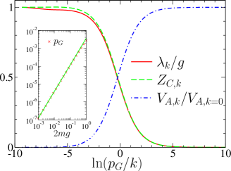
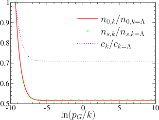
Figure 2: (Color online) $\lambda_{k}$, $Z_{C,k}$ and $V_{A,k}$ vs $\ln(p_{G}/k)$ where $p_{G}=\sqrt{(gm)^{3}\bar{n}}/4\pi$ for $\bar{n}=0.01$, $2mg=0.1$ and $d=2$ [$\ln(p_{G}/p_{c})\simeq-5.87$]. The inset shows $p_{G}$ vs $2mg$ obtained from the criterion $V_{A,p_{G}}=V_{A,k=0}/2$ [the Green solid line is a fit to $p_{G}\sim(2mg)^{3/2}$].

Figure 3: (Color online) Condensate density $n_{0,k}$, superfluid density $n_{s,k}$ and Goldstone mode velocity $c_{k}$ vs $\ln(p_{G}/k)$. The parameters are the same as in Fig. 3.

The suppression of $Z_{C,k}$, together with a finite value of $V_{A,k=0}$ shows that the average effective action (42) exhibits a “relativistic” invariance in the infrared limit and therefore becomes equivalent to that of the classical O(2) model in dimensions $d+1$. In the ordered phase, the coupling constant of this model vanishes as $\lambda_{k}\sim k^{4-(d+1)}$ Dupuis10 , which is nothing but our starting assumption (44). For $k\to 0$, the existence of a linear spectrum is due to the relativistic form of the average effective action (rather than a non-zero value of $\lambda_{k}n_{0,k}$ as in the Bogoliubov approximation) not (b).

To obtain the $k=0$ limit of the propagators (at fixed $p$), one should in principle stop the flow when $k\sim\sqrt{{\bf p}^{2}+\omega^{2}/c^{2}}$. Since thermodynamic quantities are not expected to flow in the infrared limit, they can be approximated by their $k=0$ values. As for the longitudinal correlation function, its value is obtained from the replacement $\lambda_{k}\to C(\omega^{2}+c^{2}{\bf p}^{2})^{(3-d)/2}$ (with $C$ a constant). From (45) and (47), we then deduce the exact infrared behavior of the normal and anomalous propagators (at $k=0$),

$$\begin{split}G_{\rm n}(p)={}&-\frac{n_{0}mc^{2}}{\bar{n}}\frac{1}{\omega^{2}+c^{2}{\bf p}^{2}}\\ &-\frac{mc^{2}}{\bar{n}}\frac{dn_{0}}{d\mu}\frac{i\omega}{\omega^{2}+c^{2}{\bf p}^{2}}-\frac{1}{2}G_{11}(p),\\ G_{\rm an}(p)={}&\frac{n_{0}mc^{2}}{\bar{n}}\frac{1}{\omega^{2}+c^{2}{\bf p}^{2}}-\frac{1}{2}G_{11}(p),\end{split}$$ (50)

where

$$G_{11}(p)=\frac{1}{2n_{0}C(\omega^{2}+c^{2}{\bf p}^{2})^{(3-d)/2}}.$$ (51)

The hydrodynamic approach of Sec. III correctly predicts the leading terms of (50) but approximates $dn_{0}/d\mu$ by $\bar{n}/mc^{2}$. On the other hand, it gives an explicit expression of the coefficient $C$ in the longitudinal correlation function (51).

IV.2 RG flows

The conclusions of the preceding section can be obtained more rigorously from the RG equation (40) satisfied by the average effective action. The flow of $\lambda_{k}$, $Z_{C,k}$ and $V_{A,k}$ is shown in Fig. 3 for a two-dimensional system in the weak-coupling limit. We clearly see that the Bogoliubov approximation breaks down at a characteristic momentum scale $p_{G}\sim\sqrt{(gm)^{3}\bar{n}}$. In the Goldstone regime $k\ll p_{G}$, we find that both $\lambda_{k}$ and $Z_{C,k}$ vanish linearly with $k$ in agreement with the conclusions of Sec. IV.1. Furthermore, $V_{A,k}$ takes a finite value in the limit $k\to 0$ in agreement with the limiting value (49) of the Goldstone mode velocity. Figure 3 shows the behavior of the condensate density $n_{0,k}$, the superfluid density $n_{s,k}=Z_{A,k}n_{0,k}$ and the velocity $c_{k}$. Since $Z_{A,k=0}\simeq 1.004$, the mean boson density $\bar{n}_{k}=n_{s,k}$ is nearly equal to the condensate density $n_{0,k}$. Apart from a slight variation at the beginning of the flow, $n_{0,k}$, $n_{s,k}=Z_{A,k}n_{0,k}$ and $c_{k}$ do not change with $k$. In particular, they are not sensitive to the Ginzburg scale $p_{G}$. This result is quite remarkable for the Goldstone mode velocity $c_{k}$, whose expression (46) involves the parameters $\lambda_{k}$, $Z_{C,k}$ and $V_{A,k}$, which all strongly vary when $k\sim p_{G}$. These findings are a nice illustration of the fact that the divergence of the longitudinal susceptibility does not affect local gauge invariant quantities Pistolesi et al. (2004); Dupuis (2009b).

V The superfluid–Mott-insulator transition

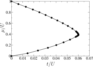
Figure 4: Phase diagram of the two-dimensional Bose-Hubbard model obtained from the NPRG Rancon10 showing the first Mott lob corresponding to a density $\bar{n}=1$.

The Bose-Hubbard model describes bosons on a $d$-dimensional lattice with Hamiltonian Fisher et al. (1989)

$$\hat{H}={} -t\sum_{\langle{\bf r},{\bf r}^{\prime}\rangle}\left(\hat{\psi}^{\dagger}_{\bf r}\hat{\psi}_{{\bf r}^{\prime}}+{\rm h.c.}\right)-\mu\sum_{\bf r}\hat{n}_{\bf r}$$

$$+\frac{U}{2}\sum_{\bf r}\hat{n}_{\bf r}(\hat{n}_{\bf r}-1),$$ (52)

where $\hat{\psi}_{\bf r}^{(\dagger)}$ is a creation/annihilation operator defined at the lattice site ${\bf r}$, $\langle{\bf r},{\bf r}^{\prime}\rangle$ denotes nearest-neighbor sites, and $\hat{n}_{\bf r}=\hat{\psi}^{\dagger}_{\bf r}\hat{\psi}_{\bf r}$. This model can be studied within the NPRG framework using a formulation adapted to lattice models Machado10 ; Rancon10 . Here we focus on the critical behavior at the superfluid–Mott-insulator transition. In the low-energy limit, we can take the continuum limit and express the average effective action as

$$\Gamma_{k}[\phi^{*},\phi]=\int_{0}^{\beta}d\tau\int d^{d}r\bigl{[} \phi^{*}(Z_{C,k}{\partial_{\tau}}-V_{A,k}\partial^{2}_{\tau}$$

$$-Z_{A,k}t\boldsymbol{\nabla}^{2})\phi+V_{k}(n)\bigr{]},$$ (53)

where $n({\bf r},\tau)=|\phi({\bf r},\tau)|^{2}$ and $\phi({\bf r},\tau)=\langle\psi({\bf r},\tau)\rangle$ denotes the superfluid order parameter. Near the transition, we can expand the effective potential $V_{k}(n)$ about $n=0$,

$$V_{k}(n)=V_{k}(0)+\delta_{k}n+\frac{\lambda_{k}}{2}n^{2}.$$ (54)

The transition line in the $(t/U,\mu/U)$ plane is defined by $\delta\equiv\delta_{k=0}=0$ (Fig. 4). The condensate density $n_{0}\equiv n_{0,k=0}$ is obtained from the minimum of $V(n)\equiv V_{k=0}(n)$. In the Mott phase ($\delta\geq 0$), $n_{0}$ vanishes while $n_{0}=-\delta/\lambda$ in the superfluid phase ($\delta\leq 0$). The mean boson density (i.e. the mean number of bosons per site) is given by

$$\bar{n} =-\frac{d}{d\mu}V(n_{0})$$

$$=\left\{\begin{array}[]{lc}-\frac{dV(0)}{d\mu}&\mbox{(insulator)},\\ -\frac{dV(0)}{d\mu}+\frac{\delta}{\lambda}\frac{d\delta}{d\mu}-\frac{\delta^{2}}{2\lambda^{2}}\frac{d\lambda}{d\mu}&\mbox{(superfluid)}.\end{array}\right.$$ (57)

In the Mott phase, the density $-dV(0)/d\mu$ is pinned to an integer value.

The existence of two universality classes at the quantum phase transition between the superfluid and the Mott insulator follows from symmetry arguments Sachdev (1999). The last of the Ward identities (47), which is associated to (local) gauge invariance Dupuis (2009b), can be expressed as

$$Z_{C}=-\frac{d\delta}{d\mu}+\frac{\delta}{\lambda}\frac{d\lambda}{d\mu}$$ (58)

in the superfluid phase. At the tip of the Mott lob where both $\delta$ and $d\delta/d\mu$ vanish, $Z_{C}$ vanishes. The effective action $\Gamma_{k=0}$ then exhibits a “relativistic” invariance and we expect the transition to be in the universality class of the $(d+1)$-dimensional $XY$ model with a dynamical exponent $z=1$. According to (57), the lob tip ($\delta=d\delta/d\mu=0$) corresponds to a transition taking place at constant density. Away from the tip, the transition is accompanied by a change in density. $Z_{C}$ is finite and the transition is mean-field like for $d\geq 2$ with $z=2$ (with logarithmic corrections for $d=2$) Sachdev (1999).

		$Z_{A,k}$	$V_{A,k}$	$Z_{C,k}$	$\lambda_{k}$	$n_{0,k}$
superfluid		$Z_{A}^{*}$	$V_{A}^{*}$	$k$	$k$	$n_{0}^{*}$
critical	$XY$	$k^{-\eta}$	$k^{-\eta}$	$k$	$k^{1-2\eta}$	$k^{1+\eta}$
behavior	mean-field	$Z_{A}^{*}$	$V_{A}^{*}$	$Z_{C}^{*}$	$|\ln k|^{-1}$	$k^{2}|\ln k|^{-1}$
insulator		$Z_{A}^{*}$	$V_{A}^{*}$	$Z_{C}^{*}$	$\lambda^{*}$	0

Table 1: Critical behavior at the superfluid–Mott-insulator transition and infrared behavior in the superfluid and Mott-insulator phases ($d=2$). The stared quantities indicate nonzero fixed-point values and $\eta$ denotes the anomalous dimension at the three-dimensional $XY$ critical point.

Table 1 summarizes the results obtained for the two-dimensional Bose-Hubbard model Rancon10 . The NPRG provides a natural explanation for the critical behavior in the $XY$ universality class which is observed when the transition takes place at constant density (tip of the Mott lob). Indeed, since the infrared behavior in the superfluid phase is characterized by a relativistic symmetry, it is not surprising that this symmetry remains at the transition to the Mott insulator. By contrast, the Bogoliubov fixed point, which has a dynamical exponent $z=2$, is clearly a poor starting point to understand the superfluid–Mott-insulator transition at the lob tip.

VI Conclusion

Interacting bosons at zero temperature are characterized by two momentum scales: the healing (or hydrodynamic) scale $p_{c}$ and the Ginzburg scale $p_{G}$. For momenta $|{\bf p}|\ll p_{c}$, it is possible to use a hydrodynamic description in terms of density and phase variables. This description allows us to derive the correlation functions of the order parameter field without encountering infrared divergences. In the Goldstone regime $|{\bf p}|,|\omega|/c\ll p_{G}$, density fluctuations play no role any more and both the transverse and longitudinal correlation functions are fully determined by transverse (phase) fluctuations. In this momentum and frequency range, the coupling between transverse and longitudinal fluctuations leads to a divergence of the longitudinal susceptibility and singular self-energies. Nevertheless, in the weak-coupling limit, the Bogoliubov theory applies to a large part of the spectrum where the dispersion is linear ($|{\bf p}|\lesssim p_{c}$) and breaks down only at very small momenta $|{\bf p}|\lesssim p_{G}\ll p_{c}$. Moreover, thermodynamic quantities are not sensitive to the Ginzburg scale $p_{G}$ and can be deduced from the Bogoliubov approach.

A direct computation of the order parameter correlation function (without relying on the hydrodynamic description) is possible, but one then has to solve the problem of infrared divergences which appear in perturbation theory when $|{\bf p}|\lesssim p_{G}$ and signal the breakdown of the Bogoliubov approximation. The NPRG provides a natural framework for such a calculation. It shows that in the Goldstone regime $|{\bf p}|,|\omega|/c\ll p_{G}$, the system is described by an effective action with relativistic invariance similar to that of the $(d+1)$-dimensional classical O(2) model. This similarity sheds light on the critical behavior of the superfluid–Mott-insulator transition in the Bose-Hubbard model which belongs to the $XY$ universality class when the transition takes place at fixed density.

References

- Bogoliubov (1947) N. N. Bogoliubov, J. Phys. USSR 11, 23 (1947).
- Dalfovo et al. (1999) F. Dalfovo, S. Giorgini, L. P. Pitaevskii, and S. Stringari, Rev. Mod. Phys. 71, 463 (1999).
- Leggett (2001) A. J. Leggett, 73, 307 (2001).
- Beliaev (1958a) S. T. Beliaev, Sov. Phys. JETP 7, 289 (1958a).
- Beliaev (1958b) S. T. Beliaev, Sov. Phys. JETP 7, 299 (1958b).
- Hugenholtz and Pines (1959) N. Hugenholtz and D. Pines, Phys. Rev. 116, 489 (1959).
- Gavoret and Nozières (1964) J. Gavoret and P. Nozières, Ann. Phys. (N.Y.) 28, 349 (1964).
- Nepomnyashchii and Nepomnyashchii (1975) A. A. Nepomnyashchii and Y. A. Nepomnyashchii, JETP Lett. 21, 1 (1975).
- Nepomnyashchii and Nepomnyashchii (1978) Y. A. Nepomnyashchii and A. A. Nepomnyashchii, Sov. Phys. JETP 48, 493 (1978).
- Nepomnyashchii (1983) Y. A. Nepomnyashchii, Sov. Phys. JETP 58, 722 (1983).
- Patasinskij and Pokrovskij (1973) A. Z. Patasinskij and V. L. Pokrovskij, Sov. Phys. JETP 37, 733 (1973).
- (12) N. Dupuis, Phys. Rev. E 83, 031120 (2011).
- Popov (1972) V. N. Popov, Theor. and Math. Phys. (Sov.) 11, 478 (1972).
- Popov (1983) V. N. Popov, Functional Integrals in Quantum Field Theory and Statistical Physics (Reidel, Dordrecht, Holland, 1983).
- Popov and Seredniakov (1979) V. N. Popov and A. V. Seredniakov, Sov. Phys. JETP 50, 193 (1979).
- Castellani et al. (1997) C. Castellani, C. D. Castro, F. Pistolesi, and G. C. Strinati, Phys. Rev. Lett. 78, 1612 (1997).
- Pistolesi et al. (2004) F. Pistolesi, C. Castellani, C. D. Castro, and G. C. Strinati, Phys. Rev. B 69, 024513 (2004).
- Dupuis and Sengupta (2007) N. Dupuis and K. Sengupta, Europhys. Lett. 80, 50007 (2007).
- Dupuis (2009a) N. Dupuis, Phys. Rev. Lett. 102, 190401 (2009a).
- Dupuis (2009b) N. Dupuis, Phys. Rev. A 80, 043627 (2009b).
- Wetterich (2008) C. Wetterich, Phys. Rev. B 77, 064504 (2008).
- Floerchinger and Wetterich (2008) S. Floerchinger and C. Wetterich, Phys. Rev. A 77, 053603 (2008).
- Sinner et al. (2009) A. Sinner, N. Hasselmann, and P. Kopietz, Phys. Rev. Lett. 102, 120601 (2009).
- (24) A. Sinner, N. Hasselmann, and P. Kopietz, Phys. Rev. A 82, 063632 (2010).
- Abrikosov et al. (1975) A. A. Abrikosov, L. P. Gor’kov, and I. E. Dzyaloshinski, Methods of Quantum Field Theory in Statistical Physics (Dover, 1975).
- Fetter and Walecka (2003) A. L. Fetter and J. D. Walecka, Quantum Theory of Many-Particle Systems (Dover, 2003).
- Petrov et al. (2004) D. S. Petrov, D. M. Gangardt, and G. V. Shlyapnikov, J. de Phys. IV 116, 3 (2004).
- Capogrosso-Sansone et al. (2010) B. Capogrosso-Sansone, S. Giorgini, S. Pilati, L. Pollet, N. Prokof’ev, B. Svistunov, and M. Troyer, New J. Phys. 12, 043010 (2010).
- not (a) Popov’s original approach Popov and Seredniakov (1979) also takes into account the influence of the non-hydrodynamic modes () on the low-energy behavior of the normal and anomalous propagators. These modes however do not change the final results (31,32) except for a minor modification in the expression of in three dimensions Dupuis10 .
- Weichman (1988) P. B. Weichman, Phys. Rev. B 38, 8739 (1988).
- Giorgini et al. (1992) S. Giorgini, L. Pitaevskii, and S. Stringari, Phys. Rev. B 46, 6374 (1992).
- Berges et al. (2002) J. Berges, N. Tetradis, and C. Wetterich, Phys. Rep. 363, 223 (2002).
- (33) B. Delamotte, arXiv:cond-mat/0702365.
- Wetterich (1993) C. Wetterich, Phys. Lett. B 301, 90 (1993).
- Huang and Klein (1964) K. Huang and A. Klein, Ann. Phys. (N.Y.) 30, 203 (1964).
- not (b) The emergence of the relativistic symmetry of the average effective action at low energy is connected to the singularities of the self-energies in the limit Dupuis10 . Thus we recover the fact that singular self-energies are crucial to obtain a linear spectrum in spite of the vanishing of the anomalous self-energies Nepomnyashchii and Nepomnyashchii (1975).
- Fisher et al. (1989) M. P. A. Fisher, P. B. Weichman, G. Grinstein, and D. S. Fisher, Phys. Rev. B 40, 546 (1989).
- (38) T. Machado and N. Dupuis, Phys. Rev. E 82, 041128 (2010).
- (39) A. Rançon and N. Dupuis, Phys. Rev. B 83, 172501 (2011).
- Sachdev (1999) S. Sachdev, Quantum Phase Transitions (Cambridge University, Cambridge, England, 1999).