Infrared behavior of interacting bosons at zero temperature

Abstract

We review the infrared behavior of interacting bosons at zero temperature. After a brief discussion of the Bogoliubov approximation and the breakdown of perturbation theory due to infrared divergences, we show how the non-perturbative renormalization group enables to obtain the exact infrared behavior of the correlation functions.

1 Introduction

Many of the predictions of the Bogoliubov theory of superfluidity[1] have been confirmed experimentally, in particular in ultracold atomic gases.[2, 3] Nevertheless a clear understanding of the infrared behavior of interacting bosons at zero temperature has remained a challenging theoretical issue for a long time. Early attempts to go beyond the Bogoliubov theory have revealed a singular perturbation theory plagued by infrared divergences due to the presence of the Bose-Einstein condensate and the Goldstone mode.[4, 5, 6] In the 1970s, Nepomnyashchii and Nepomnyashchii proved that the anomalous self-energy vanishes at zero frequency and momentum in dimension $d\leq 3$.[7] This exact result shows that the Bogoliubov approximation, where the linear spectrum and the superfluidity rely on a finite value of the anomalous self-energy, breaks down at low energy. As realized latter on,[8, 9] the singular perturbation theory is a direct consequence of the coupling between transverse and longitudinal fluctuations and reflects the divergence of the longitudinal susceptibility – a general phenomenon in systems with a continuous broken symmetry.[10]

In this paper, we review the infrared behavior of interacting bosons. A more detailed discussion together with a comparison to the classical O($N$) model can be found in Ref. [11]. In Sec. 2, we briefly review the Bogoliubov theory and the appearance of infrared divergences in perturbation theory. We introduce the Ginzburg momentum scale $p_{G}$ signaling the breakdown of the Bogoliubov approximation. In Sec. 3, we discuss the non-perturbative renormalization group (NPRG) and show how it enables to obtain the exact infrared behavior of the normal and anomalous single-particle propagators without encountering infrared divergences.[12, 13, 14, 15, 16, 17, 18, 19, 20]

2 Perturbation theory and breakdown of the Bogoliubov approximation

We consider interacting bosons at zero temperature with the (Euclidean) action

$$S=\int dx\left[\psi^{*}\left({\partial_{\tau}}-\mu-\frac{\boldsymbol{\nabla}^{2}}{2m}\right)\psi+\frac{g}{2}(\psi^{*}\psi)^{2}\right],$$ (1)

where $\psi(x)$ is a bosonic (complex) field, $x=({\bf r},\tau)$, and $\int dx=\int_{0}^{\beta}d\tau\int d^{d}r$. $\tau\in[0,\beta]$ is an imaginary time, $\beta\to\infty$ the inverse temperature, and $\mu$ denotes the chemical potential. The interaction is assumed to be local in space and the model is regularized by a momentum cutoff $\Lambda$. We consider a space dimension $d>1$.

Introducing the two-component field

$$\Psi(p)=\left(\begin{array}[]{c}\psi(p)\\ \psi^{*}(-p)\end{array}\right),\quad\Psi^{\dagger}(p)=\bigl{(}\psi^{*}(p),\psi(-p)\bigr{)}$$ (2)

(with $p=({\bf p},i\omega)$ and $\omega$ a Matsubara frequency), the one-particle (connected) propagator becomes a $2\times 2$ matrix whose inverse in Fourier space is given by

$$\left(\begin{array}[]{cc}i\omega+\mu-\epsilon_{\bf p}-\Sigma_{\rm n}(p)&-\Sigma_{\rm an}(p)\\ -\Sigma_{\rm an}^{*}(p)&-i\omega+\mu-\epsilon_{\bf p}-\Sigma_{\rm n}(-p)\end{array}\right),$$ (3)

where $\Sigma_{\rm n}$ and $\Sigma_{\rm an}$ are the normal and anomalous self-energies, respectively, and $\epsilon_{\bf p}={\bf p}^{2}/2m$. If we choose the order parameter $\langle\psi(x)\rangle=\sqrt{n_{0}}$ to be real (with $n_{0}$ the condensate density), then the anomalous self-energy $\Sigma_{\rm an}(p)$ is real.

2.1 Bogoliubov approximation

The Bogoliubov approximation is a Gaussian fluctuation theory about the saddle point solution $\psi(x)=\sqrt{n_{0}}=\sqrt{\mu/g}$. It is equivalent to a zero-loop calculation of the self-energies,[21, 22]

$$\Sigma_{\rm n}^{(0)}(p)=2gn_{0},\quad\Sigma_{\rm an}^{(0)}(p)=gn_{0}.$$ (4)

This yields the (connected) propagators

$$G_{\rm n}^{(0)}(p) = -\langle\psi(p)\psi^{*}(p)\rangle_{c}=\dfrac{-i\omega-\epsilon_{\bf p}-gn_{0}}{\omega^{2}+E_{\bf p}^{2}},$$

$$G_{\rm an}^{(0)}(p) = -\langle\psi(p)\psi(-p)\rangle_{c}=\dfrac{gn_{0}}{\omega^{2}+E_{\bf p}^{2}},$$ (5)

where $E_{\bf p}=[\epsilon_{\bf p}(\epsilon_{\bf p}+2gn_{0})]^{1/2}$ is the Bogoliubov quasi-particle excitation energy. When $|{\bf p}|$ is larger than the healing momentum $p_{c}=(2gmn_{0})^{1/2}$, the spectrum $E_{\bf p}\simeq\epsilon_{\bf p}+gn_{0}$ is particle-like, whereas it becomes sound-like for $|{\bf p}|\ll p_{c}$ with a velocity $c=\sqrt{gn_{0}/m}$. In the weak-coupling limit, $n_{0}\simeq\bar{n}$ ($\bar{n}$ is the mean boson density) and $p_{c}$ can equivalently be defined as $p_{c}=(2gm\bar{n})^{1/2}$. In the Bogoliubov approximation, the occurrence of a linear spectrum at low energy (which implies superfluidity according to Landau’s criterion) is due to $\Sigma_{\rm an}(p=0)$ being nonzero.

2.2 Infrared divergences and the Ginzburg scale

The lowest-order (one-loop) correction $\Sigma^{(1)}$ to the Bogoliubov result $\Sigma^{(0)}$ is divergent for $d\leq 3$. Retaining only the divergent part, we obtain

$$\Sigma_{\rm n}^{(1)}(p)\simeq\Sigma_{\rm an}^{(1)}(p)\simeq-2\frac{g^{4}n_{0}^{3}}{c^{3}}A_{d+1}\left({\bf p}^{2}+\frac{\omega^{2}}{c^{2}}\right)^{(d-3)/2}$$ (6)

if $d<3$ and

$$\Sigma_{\rm n}^{(1)}(p)\simeq\Sigma_{\rm an}^{(1)}(p)\simeq-\frac{g^{4}n_{0}^{3}}{c^{3}}A_{4}\ln\left(\frac{p^{2}_{c}}{{\bf p}^{2}+\omega^{2}/c^{2}}\right)$$ (7)

if $d=3$, where

$$A_{d}=\left\{\begin{array}[]{lcc}-\frac{2^{1-d}\pi^{1-d/2}}{\sin(\pi d/2)}\frac{\Gamma(d/2)}{\Gamma(d-1)}&\mbox{if}&d<4,\\ \frac{1}{8\pi^{2}}&\mbox{if}&d=4.\end{array}\right.$$ (8)

We can estimate the characteristic (Ginzburg) momentum scale $p_{G}$ below which the Bogoliubov approximation breaks down from the condition $|\Sigma_{\rm n}^{(1)}(p)|\sim\Sigma_{\rm n}^{(0)}(p)$ or $|\Sigma_{\rm an}^{(1)}(p)|\sim\Sigma_{\rm an}^{(0)}(p)$ for $|{\bf p}|=p_{G}$ and $|\omega|=cp_{G}$,

$$p_{G}\sim\left\{\begin{array}[]{lcc}(A_{d+1}gmp_{c})^{1/(3-d)}&\mbox{if}&d<3,\\ p_{c}\exp\left(-\frac{1}{A_{4}gmp_{c}}\right)&\mbox{if}&d=3.\end{array}\right.$$ (9)

This result can be rewritten as

$$p_{G}\sim\left\{\begin{array}[]{lcc}p_{c}(A_{d+1}\tilde{g}^{d/2})^{1/(3-d)}&\mbox{if}&d<3,\\ p_{c}\exp\left(-\frac{1}{A_{4}\sqrt{2}\tilde{g}^{3/2}}\right)&\mbox{if}&d=3,\end{array}\right.$$ (10)

where

$$\tilde{g}=gm\bar{n}^{1-2/d}\sim\left(\frac{p_{c}}{\bar{n}^{1/d}}\right)^{2}$$ (11)

is the dimensionless coupling constant obtained by comparing the mean interaction energy per particle $g\bar{n}$ to the typical kinetic energy $1/m\bar{r}^{2}$ where $\bar{r}\sim\bar{n}^{-1/d}$ is the mean distance between particles.[23] A superfluid is weakly correlated if $\tilde{g}\ll 1$, i.e. $p_{G}\ll p_{c}\ll\bar{n}^{1/d}$ (the characteristic momentum scale $\bar{n}^{1/d}$ does however not play any role in the weak-coupling limit). In this case, the Bogoliubov theory applies to a large part of the spectrum where the dispersion is linear (i.e. $|{\bf p}|\lesssim p_{c}$) and breaks down only at very small momenta $|{\bf p}|\lesssim p_{G}\ll p_{c}$. When the dimensionless coupling $\tilde{g}$ becomes of order unity, the three characteristic momentum scales $p_{G}\sim p_{c}\sim\bar{n}^{1/d}$ become of the same order. The momentum range $[p_{G},p_{c}]$ where the linear spectrum can be described by the Bogoliubov theory is then suppressed. We expect the strong-coupling regime $\tilde{g}\gg 1$ to be governed by a single characteristic momentum scale, namely $\bar{n}^{1/d}$.[24]

2.3 Vanishing of the anomalous self-energy

The exact values of $\Sigma_{\rm n}(p=0)$ and $\Sigma_{\rm an}(p=0)$ can be obtained using the U(1) symmetry of the action, i.e. the invariance under the field transformation $\psi(x)\to e^{i\theta}\psi(x)$ and $\psi^{*}(x)\to e^{-i\theta}\psi^{*}(x)$. On the one hand, the self-energies satisfy the Hugenholtz-Pines theorem,[4]

$$\Sigma_{\rm n}(p=0)-\Sigma_{\rm an}(p=0)=\mu.$$ (12)

On the other hand, the anomalous self-energy vanishes,

$$\Sigma_{\rm an}(p=0)=0.$$ (13)

The last result was first proven by Nepomnyashchii and Nepomnyashchii.[7, 20, 11] It shows that the Bogoliubov theory, where the linear spectrum and the superfluidity rely on a finite value of the anomalous self-energy, breaks down at low energy in agreement with the conclusions drawn from perturbation theory (Sec. 2.2).

3 The non-perturbative RG

The NPRG enables to circumvent the difficulties of perturbation theory and derive the correlation functions in the low-energy limit.[12, 13, 16, 17, 18, 14, 15, 19, 20] The strategy of the NPRG is to build a family of theories indexed by a momentum scale $k$ such that fluctuations are smoothly taken into account as $k$ is lowered from the microscopic scale $\Lambda$ down to 0.[25, 26] This is achieved by adding to the action (1) an infrared regulator term

$$\Delta S_{k}[\psi^{*},\psi]=\sum_{p}\psi^{*}(p)R_{k}(p)\psi(p).$$ (14)

The main quantity of interest is the so-called average effective action

$$\Gamma_{k}[\phi^{*},\phi]=-\ln Z_{k}[J^{*},J]+\sum_{p}[J^{*}(p)\phi(p)+{\rm c.c.}]-\Delta S_{k}[\phi^{*},\phi],$$ (15)

defined as a modified Legendre transform of $-\ln Z_{k}[J^{*},J]$ which includes the subtraction of $\Delta S_{k}[\phi^{*},\phi]$. $J$ denotes a complex external source that couples linearly to the boson field $\psi$ and $\phi(x)=\langle\psi(x)\rangle$ is the superfluid order parameter. The cutoff function $R_{k}$ is chosen such that at the microscopic scale $\Lambda$ it suppresses all fluctuations, so that the mean-field approximation $\Gamma_{\Lambda}[\phi^{*},\phi]=S[\phi^{*},\phi]$ becomes exact. The effective action of the original model (1) is given by $\Gamma_{k=0}$ provided that $R_{k=0}$ vanishes. For a generic value of $k$, the cutoff function $R_{k}(p)$ suppresses fluctuations with momentum $|{\bf p}|\lesssim k$ and frequency $|\omega|\lesssim ck$ but leaves those with $|{\bf p}|,|\omega|/c\gtrsim k$ unaffected ($c\equiv c_{k}$ is the velocity of the Goldstone mode). The dependence of the average effective action on $k$ is given by Wetterich’s equation[28]

$$\partial_{t}\Gamma_{k}[\phi^{*},\phi]=\frac{1}{2}{\rm Tr}\left\{\dot{R}_{k}\left(\Gamma^{(2)}_{k}[\phi^{*},\phi]+R_{k}\right)^{-1}\right\},$$ (16)

where $t=\ln(k/\Lambda)$ and $\dot{R}_{k}=\partial_{t}R_{k}$. $\Gamma^{(2)}_{k}[\phi^{*},\phi]$ denotes the second-order functional derivative of $\Gamma_{k}[\phi]$. In Fourier space, the trace involves a sum over momenta and frequencies as well as the internal index of the $\phi$ field.

3.1 Derivative expansion and infrared behavior

Because of the regulator term $\Delta S_{k}$, the vertices $\Gamma^{(n)}_{k}(p_{1},\cdots,p_{n})$ are smooth functions of momenta and frequencies and can be expanded in powers of ${\bf p}_{i}^{2}/k^{2}$ and $\omega_{i}^{2}/c^{2}k^{2}$. Thus if we are interested only in the low-energy properties, we can use a derivative expansion of the average effective action.[25, 26] In the following we consider the ansatz[27]

$$\Gamma_{k}[\phi^{*},\phi]=\int dx\Bigl{[}\phi^{*}\Bigl{(}Z_{C,k}{\partial_{\tau}}-V_{A,k}\partial^{2}_{\tau}-\frac{Z_{A,k}}{2m}\boldsymbol{\nabla}^{2}\Bigr{)}\phi+\frac{\lambda_{k}}{2}(n-n_{0,k})^{2}\Bigr{]},$$ (17)

where $n=|\phi|^{2}$. $n_{0,k}$ denotes the condensate density in the equilibrium state. We have introduced a second-order time derivative term. Although not present in the initial average effective action $\Gamma_{\Lambda}$, we shall see that this term plays a crucial role when $d\leq 3$.[14, 16]

In a broken U(1) symmetry state with real order parameter $\phi=\sqrt{n_{0}}$, the normal and anomalous self-energies are given by

$$\Sigma_{k,{\rm n}}(p) = \mu+V_{A,k}\omega^{2}+(1-Z_{C,k})i\omega-(1-Z_{A,k})\epsilon_{\bf p}+\lambda_{k}n_{0,k},$$ (18)

$$\Sigma_{k,{\rm an}}(p) = \lambda_{k}n_{0,k}.$$

These expressions imply the existence of a sound mode with velocity

$$c_{k}=\left(\frac{Z_{A,k}/2m}{V_{A,k}+Z_{C,k}^{2}/2\lambda_{k}n_{0,k}}\right)^{1/2}.$$ (19)

At the initial stage of the flow, $Z_{A,\Lambda}=Z_{C,\Lambda}=1$, $V_{A,\Lambda}=0$, $\lambda_{\Lambda}=g$ and $n_{0,\Lambda}=\mu/g$, which reproduces the results of the Bogoliubov approximation. A crucial property of the RG flow is that

$$\lambda_{k}\sim k^{3-d}$$ (20)

vanishes with $k$ when $d\leq 3$. Eq. (20) follows from the numerical solution of the RG equations, but can also be anticipated from the expected singular behavior of the longitudinal propagator.[11]

The parameters $Z_{A,k}$, $Z_{C,k}$ and $V_{A,k}$ can be related to thermodynamic quantities using Ward identities,[5, 13, 18]

$$n_{s,k} = Z_{A,k}n_{0,k}=\bar{n}_{k},$$

$$V_{A,k} = -\frac{1}{2n_{0,k}}\frac{\partial^{2}U_{k}}{\partial\mu^{2}}\biggl{|}_{n_{0,k}},$$ (21)

$$Z_{C,k} = -\frac{\partial^{2}U_{k}}{\partial n\partial\mu}\biggl{|}_{n_{0,k}}=\lambda_{k}\frac{dn_{0,k}}{d\mu},$$

where $\bar{n}_{k}$ is the mean boson density and $n_{s,k}$ the superfluid density. Here we consider the effective potential $U_{k}$ as a function of the two independent variables $n$ and $\mu$. The first of equations (21) states that in a Galilean invariant superfluid at zero temperature, the superfluid density is given by the full density of the fluid.[5] Equations (21) also imply that the Goldstone mode velocity $c_{k}$ coincides with the macroscopic sound velocity,[5, 13, 18] i.e.

$$\frac{d\bar{n}_{k}}{d\mu}=\frac{\bar{n}_{k}}{mc_{k}^{2}}.$$ (22)

Since thermodynamic quantities, including the condensate “compressibility” $dn_{0,k}/d\mu$ should remain finite in the limit $k\to 0$, we deduce from (21) that $Z_{C,k}\sim\lambda_{k}\sim k^{3-d}$ vanishes in the infrared limit, and

$$\lim_{k\to 0}c_{k}=\lim_{k\to 0}\left(\frac{Z_{A,k}}{2mV_{A,k}}\right)^{1/2}.$$ (23)

Both $Z_{A,k}=\bar{n}_{k}/n_{0,k}$ and the macroscopic sound velocity $c_{k}$ being finite at $k=0$, $V_{A,k}$ (which vanishes in the Bogoliubov approximation) takes a non-zero value when $k\to 0$.

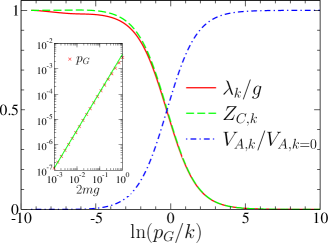
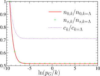
Figure 1: (Color online) (Left panel) $\lambda_{k}$, $Z_{C,k}$ and $V_{A,k}$ vs $\ln(p_{G}/k)$ where $p_{G}=\sqrt{(gm)^{3}\bar{n}}/4\pi$ for $\bar{n}=0.01$, $2mg=0.1$ and $d=2$ [$\ln(p_{G}/p_{c})\simeq-5.87$]. The inset shows $p_{G}$ vs $2mg$ obtained from the criterion $V_{A,p_{G}}=V_{A,k=0}/2$ [the Green solid line is a fit to $p_{G}\sim(2mg)^{3/2}$]. (Right panel) Condensate density $n_{0,k}$, superfluid density $n_{s,k}$ and Goldstone mode velocity $c_{k}$ vs $\ln(p_{G}/k)$.

The suppression of $Z_{C,k}$, together with a finite value of $V_{A,k=0}$ shows that the average effective action (17) exhibits a “relativistic” invariance in the infrared limit and therefore becomes equivalent to that of the classical O(2) model in dimensions $d+1$. In the ordered phase, the coupling constant of this model vanishes as $\lambda_{k}\sim k^{4-(d+1)}$,[11] which agrees with (20). For $k\to 0$, the existence of a linear spectrum is due to the relativistic form of the average effective action (rather than a non-zero value of $\lambda_{k}n_{0,k}$ as in the Bogoliubov approximation).

To obtain the $k=0$ limit of the propagators (at fixed $p$), one should in principle stop the flow when $k\sim\sqrt{{\bf p}^{2}+\omega^{2}/c^{2}}$.[18] Since thermodynamic quantities are not expected to flow in the infrared limit, they can be approximated by their $k=0$ values. Making use of the Ward identities (21), we deduce the exact infrared behavior of the normal and anomalous propagators (at $k=0$),[18]

$$G_{\rm n}(p) = -\frac{n_{0}mc^{2}}{\bar{n}}\frac{1}{\omega^{2}+c^{2}{\bf p}^{2}}-\frac{mc^{2}}{\bar{n}}\frac{dn_{0}}{d\mu}\frac{i\omega}{\omega^{2}+c^{2}{\bf p}^{2}}-\frac{1}{2}G_{\parallel}(p),$$

$$G_{\rm an}(p) = \frac{n_{0}mc^{2}}{\bar{n}}\frac{1}{\omega^{2}+c^{2}{\bf p}^{2}}-\frac{1}{2}G_{\parallel}(p),$$ (24)

where

$$G_{\parallel}(p)=\frac{1}{2n_{0}C(\omega^{2}+c^{2}{\bf p}^{2})^{(3-d)/2}}$$ (25)

is the propagator of the longitudinal fluctuations. The constant $C$ follows from the replacement $\lambda_{k}\to C(\omega^{2}+c^{2}{\bf p}^{2})^{(3-d)/2}$. The leading terms in (24) agree with the results of Gavoret and Nozières.[5] The contribution of the diverging longitudinal correlation function was first identified by Nepomnyashchii and Nepomnyashchii.[8, 9]

3.2 RG flows

The conclusions of the preceding section can be obtained more rigorously from the RG equation (16) satisfied by the average effective action. The flow of $\lambda_{k}$, $Z_{C,k}$ and $V_{A,k}$ is shown in Fig. 1 for a two-dimensional system in the weak-coupling limit. We clearly see that the Bogoliubov approximation breaks down at a characteristic momentum scale $p_{G}\sim\sqrt{(gm)^{3}\bar{n}}$. In the Goldstone regime $k\ll p_{G}$, we find that both $\lambda_{k}$ and $Z_{C,k}$ vanish linearly with $k$ in agreement with the conclusions of Sec. 3.1. Furthermore, $V_{A,k}$ takes a finite value in the limit $k\to 0$ in agreement with the limiting value (23) of the Goldstone mode velocity. Figure 1 also shows the behavior of the condensate density $n_{0,k}$, the superfluid density $n_{s,k}=Z_{A,k}n_{0,k}$ and the velocity $c_{k}$. Since $Z_{A,k=0}\simeq 1.004$, the mean boson density $\bar{n}_{k}=n_{s,k}$ is nearly equal to the condensate density $n_{0,k}$. Apart from a slight variation at the beginning of the flow, $n_{0,k}$, $n_{s,k}=Z_{A,k}n_{0,k}$ and $c_{k}$ do not change with $k$. In particular, they are not sensitive to the Ginzburg scale $p_{G}$. This result is quite remarkable for the Goldstone mode velocity $c_{k}$, whose expression (19) involves the parameters $\lambda_{k}$, $Z_{C,k}$ and $V_{A,k}$, which all strongly vary when $k\sim p_{G}$. These findings are a nice illustration of the fact that the divergence of the longitudinal susceptibility does not affect local gauge invariant quantities.[13, 18]

4 Conclusion

Interacting bosons at zero temperature are characterized by two momentum scales: the healing (or hydrodynamic) scale $p_{c}$ and the Ginzburg scale $p_{G}$. $p_{G}$ sets the scale at which the Bogoliubov approximation breaks down. For momenta $|{\bf p}|\ll p_{c}$, it is possible to use a hydrodynamic description in terms of density and phase variables. This description allows one to compute the correlation functions without encountering infrared divergences.[29, 11] In this paper, we have reviewed another approach, based on the NPRG, which enables to describe the system at all energy scales and yields the exact infrared behavior of the single-particle propagator. A nice feature of the NPRG is that it can be used to study models of strongly-correlated bosons such as the Bose-Hubbard model.[30]

References

- [1] N. N. Bogoliubov, J. Phys. USSR 11, 23 (1947).
- [2] F. Dalfovo, S. Giorgini, L. P. Pitaevskii, and S. Stringari, Rev. Mod. Phys. 71, 463 (1999).
- [3] A. J. Leggett, Rev. Mod. Phys. 73, 307 (2001).
- [4] N. M. Hugenholtz and D. Pines, Phys. Rev. 116, 489 (1959).
- [5] J. Gavoret and P. Nozières, Ann. Phys. (N.Y.) 28, 349 (1964).
- [6] S. T. Beliaev, Sov. Phys. JETP 7, 289 (1958); Sov. Phys. JETP, 7, 299 (1958).
- [7] A. A. Nepomnyashchii and Yu. A. Nepomnyashchii, JETP Lett. 21, 1 (1975).
- [8] Yu. A. Nepomnyashchii and A. A. Nepomnyashchii, Sov. Phys. JETP 48, 493 (1978).
- [9] Yu. A. Nepomnyashchii, Sov. Phys. JETP 58, 722 (1983).
- [10] A. Z. Patasinskij and V. L. Pokrovskij, Sov. Phys. JETP 37, 733 (1973).
- [11] N. Dupuis, Phys. Rev. E 83, 031120 (2011)
- [12] C. Castellani, C. Di Castro, F. Pistolesi, and G. C. Strinati, Phys. Rev. Lett. 78, 1612 (1997).
- [13] F. Pistolesi, C. Castellani, C. Di Castro, and G. C. Strinati, Phys. Rev. B 69, 024513 (2004).
- [14] C. Wetterich, Phys. Rev. B 77, 064504 (2008).
- [15] S. Floerchinger and C. Wetterich, Phys. Rev. A 7, 053603 (2008).
- [16] N. Dupuis and K. Sengupta, Europhys. Lett. 80, 50007 (2007).
- [17] N. Dupuis, Phys. Rev. Lett. 102, 190401 (2009).
- [18] N. Dupuis, Phys. Rev. A 80, 043627 (2009).
- [19] A. Sinner, N. Hasselmann, and P. Kopietz, Phys. Rev. Lett. 102, 120601 (2009).
- [20] A. Sinner, N. Hasselmann, and P. Kopietz, Phys. Rev. A 82, 063632 (2010).
- [21] A. A. Abrikosov, L. P. Gor’kov, and I. E. Dzyaloshinski, Methods of Quantum Field Theory in Statistical Physics (Dover, 1975).
- [22] A. L. Fetter and J. D. Walecka, Quantum Theory of Many-Particle Systems (Dover, 2003).
- [23] D. S. Petrov, D. M. Gangardt, and G. V. Shlyapnikov, J. de Phys. IV 116, 5 (2004).
- [24] Note however that in the strong-coupling limit (i.e. in three dimensions, with the -wave scattering length), the bound states of the interaction potential cannot be ignored. As a result, stability is not guaranteed and the system is at best in a quasistable state: see E. Braaten, H.-W. Hammer, and T. Mehen, Phys. Rev. Lett. 88, 040401 (2002). The strong-coupling limit of interacting bosons can nevertheless be reached in the Bose-Hubbard model.[30]
- [25] J. Berges, N. Tetradis, and C. Wetterich, Phys. Rep. 363, 223 (2002).
- [26] B. Delamotte, arXiv:cond-mat/0702365.
- [27] One could consider a more general ansatz where , and are functions of the condensate density , and the full effective potential is retained rather than expanded to quadratic order about . In the superfluid phase, is convex but otherwise the conclusions regarding the infrared behavior are unchanged.
- [28] C. Wetterich, Phys. Lett. B 301, 90 (1993).
- [29] V. N. Popov and A. V. Seredniakov, Sov. Phys. JETP 50, 193 (1979).
- [30] A. Rançon and N. Dupuis, Phys. Rev. B 83, 172501 (2011).