Magnetocardiography with a modular spin-exchange relaxation free atomic magnetometer array

Abstract

We present a portable four-channel atomic magnetometer array operating in the spin exchange relaxation-free regime. The magnetometer array has several design features intended to maximize its suitability for biomagnetic measurement, specifically foetal magnetocardiography, such as a compact modular design and fibre coupled lasers. The modular design allows the independent positioning and orientation of each magnetometer. Using this array in a magnetically shielded room, we acquire adult magnetocadiograms. These measurements were taken with a 6–11 fT Hz^-1/2 single-channel baseline sensitivity that is consistent with the independently measured noise level of the magnetically shielded room.

Keywords: Instrumentation and measurement, Atomic and molecular physics, Medical physics, Biological physics

1 Introduction

Human biomagnetism has been an important area of fundamental research and medicine since the first low noise studies by ?. Magnetic signals can provide complimentary or unique information in several applications, such as magnetoencephalography (MEG) (?) and magnetocardiography (MCG) (?). For example, high quality foetal MCG (fMCG) signals can direct in utero diagnosis and therapy of cardiac arrhythmia such as supraventricular tachycardia and torsades de pointes (?, ?).

Typically, these studies use superconducting quantum interference devices (SQUIDs) for magnetic field detection, usually operated in arrays of matched gradiometers with 30 or more channels. SQUIDs have achieved a noise limit of around 1 fT Hz^-1/2 (?), but they are expensive and require liquid ⁴He for the low T_c systems for the high signal-to-noise ratio (SNR) needed for demanding biomagnetic applications like fMCG (?).

Atomic magnetometers have recently shown promise for use in biomagnetism. Atomic vapor magnetometers operating in the spin exchange relaxation free (SERF) regime (?) have recently surpassed the sensitivity of SQUID systems, achieving 160 aT Hz^-1/2 sensitivities (?). Additionally, the application of microfabrication techniques to the manufacture of mm-scale alkali-metal vapor cells and integrated fibre-coupled optics (?) allows the possibility of large arrays of SERF magnetometers, similar to current commercial SQUID systems. Besides offering increased sensitivity, atomic magnetometers are operated at temperatures between 25–180 C (?), replacing expensive cryogenics and maintenance of SQUID systems with simple resistive electrical heating and passive thermal insulation.

In this paper, we report a four-channel portable atomic magnetometer array suited for biomagnetic applications. Each magnetometer in the array features a 6–11 fT Hz^-1/2 noise floor from 10–100 Hz and has adjustable channel spacing and orientation. All channels are self-contained, including local tri-axial nulling coils, in principle allowing the channels to be placed in an arbitrarily oriented non-planar geometry. Using this array in a magnetically shielded room (MSR), we have made high quality adult MCG measurements to demonstrate the efficacy of our device for use with human subjects.

Previously, adult MEG has been measured using a similar sized fibre coupled atomic magnetometer operating in a different detection mode (?). Single channel sensitivity was comparable to ours, but quadrant photodiode detection was used to construct gradiometer signals, rather than the use of multiple magnetometers. A similar technique using a photodiode array was used previously (?), but with a large non-portable setup. In both cases, the separation between photodiode elements is small compared the the signal source depth of an MCG measurement. In this regime, the individual sensors will measure approximately the same signal, and will not operate as truly multichannel devices on their own.

Adult MCG studies have also been performed. ? used an array of 25 room temperature Cs (non-SERF mode) magnetometers as a 19-channel set of 2nd order gradiometers to map adult MCG in an eddy-current shield. They were able to suppress the noise by a factor of 1000 using this technique, but were limited to 300 fT Hz^-1/2 in this configuration.

Recently, ? used a single channel microfabricated mm-scale alkali-metal vapor cell to measure adult MCG in an MSR. Their signals compare well with SQUIDs simultaneously measuring the MCG. The measurements were performed with a sensitivity 100-200 fT Hz^-1/2 but in a much quieter shielded room (?). Results from a single magnetometer were presented.

The outline of the rest of the paper is as follows: in section 2, we summarize the theory of operation of our SERF magnetometer. Section 3 presents our apparatus and design features. Section 4 details the operation and characterization procedure of our array. In section 5, we show a sample adult MCG, compare our measured QRS amplitudes from 13 subjects with previous results in the literature, and demonstrate the acquisition of much smaller test signals applied with a phantom. Section 6 provides an analysis of the noise sources limiting our sensitivity. Finally, section 7 concludes with directions for future work towards the goal of obtaining fMCG signals.

2 Theory

The magnetometer presented here operates similarly to previous SERF magnetometers such as ? and ?. Optical pumping creates a nonzero average electron spin along the propagation direction of the pumping laser. Orthogonal magnetic fields cause the population spin to precess at the slowed down Larmor frequency (?). Spin-relaxation collisions and the absorption of laser photons interrupt the precession. The balance between optical pumping, spin relaxation, and Larmor precession determines the dynamics of the atomic polarisation and the performance of the magnetometer. A probe laser detects the orthogonal components of the electron spin.

Figure 1(a) and (b) show the optical setup and ⁸⁷Rb energy level diagram, respectively. A circularly polarised pump beam resonant with the “D1” transition optically pumps the atoms. An orthogonal probe beam detuned from the “D2” transition detects atomic spin precession due to external fields using the Faraday effect and a balanced polarimeter. The polarisers at the output of the optical fibre convert laser polarisation noise into intensity noise, to which our configuration is much less sensitive.

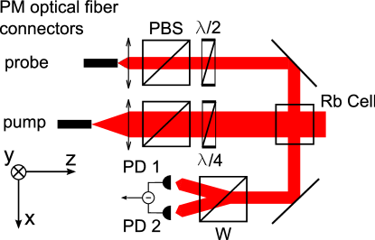
(a)

(b)

Figure 1: (a) Laser beam path schematic. The 795 nm pump laser is linearly polarised by a polarising beam splitter (PBS) and then circularly polarised by the quarter waveplate ($\lambda/4$). The 780 nm probe is detuned from the D2 resonance and linearly polarised. Both lasers are conveyed from their sources to the optics via polarisation maintaining (PM) optical fibres. The half waveplate ($\lambda/2$) is used to balance the photodiode (PD) difference signal from the Wollaston polarising beam splitter (W). (b) A simplified diagram of the first three fine-structure ⁸⁷Rb energy levels.

2.1 Polarisation equation of motion and steady state solution

We summarize here a simplified theory of operation of the magnetometer (?) to aid interpretation of our results. We use the simplifying assumption that the absorption linewidth is broad (18 GHz/(atm buffer gas)) compared to the ⁸⁷Rb ground state hyperfine splitting (6.8 GHz), though in our cells the hyperfine splitting and pressure broadening are nearly equal and the model will be approximate. If the magnetometer is operated with sufficiently high Rb density and sufficiently low total magnetic field, spin-exchange collisions preserve the coherence of the transverse spin (?) and three relaxation processes dominate the polarization relaxation rate $\Gamma$,

$$\Gamma=\Gamma_{\mathrm{sd}}+\Gamma_{\mathrm{pr}}+R,$$ (1)

where $R$ is the optical pumping rate (the rate that an unpolarised atom would absorb pump photons), $\Gamma_{\mathrm{sd}}$ is the spin-destruction rate from collisions and $\Gamma_{\mathrm{pr}}$ is the absorption rate of probe laser photons.

Assuming the Rb atoms are in spin-temperature equilibrium (?) and neglecting diffusion, the polarisation has a steady-state solution for static magnetic fields (?)

$$P_{x}=P_{z}\left(\frac{\Gamma\Omega_{y}+\Omega_{x}\Omega_{z}}{\Gamma^{2}+\Omega_{z}^{2}}\right)\approx P_{z}\frac{\Omega_{y}}{\Gamma},$$ (2)

where $\boldsymbol{\Omega}=\gamma{\bf B}$ is the Larmor frequency from a magnetic field B and $\gamma=g_{\mathrm{s}}\mu_{\mathrm{B}}/\hbar$. ${\bf P}$ is the Rb polarisation in the coordinate system of figure 1(a). The approximations on the right hand side of (2) hold for small magnetic fields such that $|\Omega|\ll\Gamma$. At typical $\Gamma\approx 2\pi\times 1000$/s, this limits B to $\ll 30$ nT.

2.2 Signal size and sensitivity

The Rb polarisation modifies the susceptibility of the atomic vapor, which changes the index of refraction for $\sigma_{+}$ and $\sigma_{-}$ circularly polarised light. For linearly polarised light, this causes a rotation of the polarisation angle. In our case, the probe beam is linearly polarised in the $\hat{y}-\hat{z}$ plane and is rotated in this plane by (?)

$$\phi\approx\frac{1}{4}r_{\mathrm{e}}fcnl\frac{(\nu-\nu_{0})}{(\nu-\nu_{0})^{2}+(\Delta\nu/2)^{2}}P_{x},$$ (3)

where $r_{\mathrm{e}}$ is the classical electron radius, $f$ is the transition oscillator strength, $c$ is the speed of light, $n$ is the Rb atomic number density, $l$ is the optical path length, $\nu-\nu_{0}$ is the probe laser detuning from the D2 resonance, and $\Delta\nu$ is the pressure broadened absorption linewidth of the transition. For reference, using our experimental parameters (see section 6), (3) evaluates to $\phi/B_{y}\approx 0.1$ $\mu$Rad/fT. For perspective, the differential photocurrent is $\Delta I=2P_{0}\epsilon\phi$, with probe laser power $P_{0}$ and a photodiode power to current conversion $\epsilon$, is around 250 pA/fT.

3 Apparatus and design considerations

3.1 Apparatus description

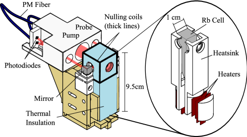
(a)

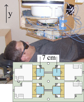
(b)

Figure 2: (a) Single magnetometer unit (left) with view inside the thermal insulation (right). Square tri-axial nulling coils are wrapped around the insulation. (b)(bottom insert) Four channel magnetometer array, with 7 cm channel spacing. This array is mounted on an existing SQUID gantry top-down, as in (b)(top). In human subject trials, the subject lays on a bed and the array is centered over the subject’s heart by equalizing the signal in all four channels in real time. The $\hat{x}$, $\hat{y}$, and $\hat{z}$ axes in the text refer to magnetometer body axes. Here, all $\hat{y}$ are aligned and correspond to the sensitive direction for all magnetometers.

Design choices in this atomic magnetometer are meant to minimize noise consistent with maximizing suitability for biomagnetic measurements. Figure 2(a) shows a single magnetometer unit. It consists of three fixed optics tubes with all the optics from the schematic in figure 1(a), a Pyrex ⁸⁷Rb vapor cell (Triad Technologies) press-fit inside a boron-nitride heatsink thermally contacted to resistive-film heaters (Minco) and a thermistor, all surrounded by thermal insulation (Aerogel). A plastic scaffold clamps the heatsink, optics tube, and two custom-made plastic mirror mounts in place. Single-turn triaxial coils are wrapped around the thermal insulation to locally null the magnetic fields in the detection volume and provide calibration and control fields. Polarisation maintaining fibres connect the optics tube to the pump and probe lasers. The pump laser is a distributed feedback type with output power 80 mW (Eagleyard Photonics), detuned $|\Delta\nu_{\mathrm{pump}}|\leq 20$ GHz from the D1 resonance. The probe laser is a 20 mW tunable external cavity diode laser (Sacher Lasertechnik Group), detuned $\sim$0.2 nm from the D2 resonance. The two lasers are each split equally into four separate fibres with an integrated polarisation maintaining splitter (Oz-Optics). The result is a set of individual magnetometer channels that are unconstrained with respect to one another, due to local fibre coupled optics and individual magnetic field control at each cell.

The lasers are mounted on a portable breadboard which, along with all the coil control electronics and monitoring equipment, fit on a single cart. A PXI based FPGA data acquisition unit (National Instruments) is used to apply calibration fields and digitize magnetometer signals. The PXI crate also houses power supply cards to control the vapor cell heaters. This modular design ensures the entire apparatus is easily transported between the MSR and our testing lab in a different building.

Material selection was aimed at minimizing Johnson noise caused by the use of electrical conductors. Each magnetometer unit shown in figure 2(a) contains only a few conductive pieces, namely the heaters, thermistor leads, optical fibre terminations, and the photodiode leads.

The vapor cell is 1 x 1 x 5 cm Pyrex rectangular container with isotopically pure ⁸⁷Rb and buffer gas composed of 50 Torr nitrogen to prevent radiation trapping (?) and 760 Torr He at the time of manufacture. Subsequent measurement showed slow loss of buffer gas pressure indicating He loss consistent with diffusion through the Pyrex cell walls (?). We estimate the data presented here was taken with a residual He pressure of $\sim$200 Torr. The cells were operated at a temperature of 140–180 C. Each magnetometer requires 4 W of heater power in thermal equilibrium, corresponding to electrical currents near 0.5 A, large enough to produce potentially disruptive magnetic fields and gradients. We manage these using matched heater pairs with oppositely aligned magnetic fields and a boron nitride heatsink to spatially separate the heaters from the detection volume of the vapor cell. Furthermore, the heater currents were modulated at 100 kHz so these magnetic fields and their gradient fields would average to zero on the time scale of MCG measurements. There is no detectable difference between the magnetic noise level with the heaters on or off.

Figure 2(b) shows a photograph of the array mounted to an existing gantry for a previously installed commercial SQUID system. Human subjects lie on a bed under the array. The array can be translated, rotated, and tilted using the gantry controls. For convenience in these initial tests, our measurements were made with planar square array and channel spacing of 7 cm. The minimum planar array spacing for all four elements is 4.5 cm. More magnetometers can be added, with 7 cm spacing in the vertical direction of figure 2(b)(bottom), while the optics tubes require the spacing in the horizontal direction to be $>$10 cm. In our setup, the four elements operate independently and could be tilted or translated with respect to one another. It should be straightforward to implement non-planar geometries.

3.2 Modularity

DC fields in the MSR, 10–50 nT, decrease the fundamental sensitivity according to (2) and require nulling. Figure 3(a) shows a sweep of $B_{y}$ and a fit with $R=400\approx\Gamma$ to (2) with $\Omega_{x},\Omega_{z}=0$. $B_{y}$ must be nulled to better than $|B_{y}|\leq 2$ nT to remain in the sensitive linear region of the response.

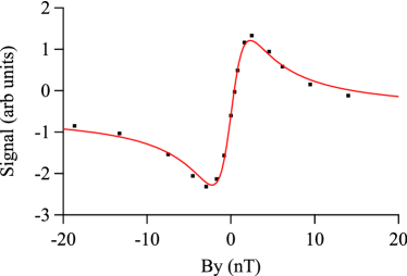
(a)

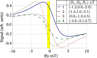
(b)

Figure 3: (a) Magnetometer signal as a function of applied field (dots) and a fit to an amplitude scaled version of (2). (b) A simulation of $P_{x}$ for multiple magnetometers in the presence of the measured magnetic field gradients from the zero values at each channel. With only a single set of tri-axial coils, these are the minimum gradients in the shielded room, and represent the best-case operating point for the four magnetometers. In this case, a compromise value for $B_{y}$ must be chosen, reducing the usable operating range. This illustrates the need for local control over the magnetic fields at each cell.

If the MSR magnetic fields were sufficiently uniform, we could use a single set of tri-axial coils with side length $a$ and array channel baseline spacing $d$ such that $a\gg d$ to simultaneously cancel the magnetic fields at all magnetometers. Having tried this, we have found two problems with this approach that resulted in the choice of small individual cancellation coils for each magnetometer.

First, residual MSR magnetic field gradients are too large on the scale of the spacing of our magnetometers to allow a uniform nulling field to be used. Figure 3(b) shows the response predicted by (2) for four magnetometers in the presence of measured MSR magnetic field gradients and $R$ from the fit in figure 3(a). $B_{x}$, $B_{y}$, and $B_{z}$ are the differences from the measured zero values at each magnetometer channel. As shown in figure 3(b), these gradients cause a decrease in both the single channel sensitivity and the effective multichannel $B_{y}$ operating range (highlighted in yellow), which has been decreased by a factor of 4 to $|B_{y}|\leq 0.5$ nT.

Second, and most importantly, the pumping laser can cause a light shift (or AC Stark shift) due to the pump laser interacting differently with different Zeeman sublevels through the Rb vector polarisability (?, ?). This causes an effective magnetic field (?)

$${\bf\Omega}_{\mathrm{LS}}\approx R\Delta\hat{s},$$ (4)

where $\Delta$ is the ratio of the laser detuning from atomic line centre to absorption linewidth, and $\hat{s}$ is the photon helicity, $\pm 1$ along the pump propagation direction for circularly polarised light.

At high optical depths corresponding to high temperatures, the pump beam is absorbed before polarising the entire cell length unless it is detuned $\Delta$ $\sim$ 1 from resonance, resulting in a nonzero ${\bf\Omega}_{\mathrm{LS}}$. The magnitude $|{\bf\Omega}_{\mathrm{LS}}|$ is roughly the same from cell to cell, but the direction with respect to the null coils depends on the orientation of the magnetometer and the direction of $\hat{s}$. For our laser parameters, we expect the pump light to cause effective fields of magnitude $\sim$ 50 nT. Orienting all the magnetometers to have the same light shift with respect to the external coils mitigates the problem, though the nonuniform light shift within each cell due to the spatial intensity profile of the laser results in a broadening of the magnetometer dispersion (?).

The light shift presents a problem for the prospects of differing individual channel orientation and tilt, or nonplanar arrays. There are also practical problems associated with large coils, such as limited magnetometer adjustment and complications with calibration fields when the magnetometers are not aligned with the coil axis. These problems are all solved by using individual sets of coils for each magnetometer.

4 Methods

4.1 Residual Field Nulling

We find the DC null fields for a single magnetometer as follows (?, ?):

• sweep $B_{y}$ and set the operating point in the centre of the dispersive curve, where the magnetometer is most sensitive.

• apply a 50 pT oscillating field $B_{0}\sin(\omega t)\hat{x}$ at 10–30 Hz and adjust $B_{z}$ until there is no response to $B_{0}$, ensuring $B_{y}$ remains at its most sensitive operating point.

• apply $B_{0}\sin(\omega t)\hat{z}$ and adjust $B_{x}$ to null the response, again ensuring $B_{y}$ is adjusted to maintain maximum sensitivity.

• repeat until residual response to $B_{x}$ and $B_{z}$ is minimized.

For the four-magnetometer array, we repeat this procedure for each individual unit. Iterating the procedure two times eliminates any offsets of the local field at the first magnetometer caused by adjusting the fields in the later ones to below the adjustment procedure sensitivity.

There is no cross-talk between our four channels because the magnetometers are fundamentally passive devices. Non-uniform light shifts from the Gaussian pump laser intensity profile cause non-uniform effective magnetic fields as in (4). Due to the residual $\Omega_{z}$ term in (2), each magnetometer retains some sensitivity to $B_{x}$. This is typically a correction of $\leq 10\%$ and its effect is ignored in what follows.

As discussed in section 3.2, the magnetometers must be within approximately 1 nT of thier null point in order to maintain uncompromised sensitivity. Background field variations in the shielded room are generally smaller by an order of magnitude or more on the timescales of of a 30 s MCG measurement. Long-term variations can take the magnetometers outside of the optimal measurement range and are easily compensated between measurements.

4.2 Magnetometer sensitivity and noise floor characterization

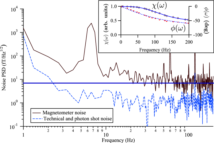
Figure 4: Measured magnetic noise (solid black) of a single characteristic magnetometer channel on a magnetically quiet day in the MSR. (Inset) Amplitude response $\chi(\omega)$ (open circles) and phase response $\phi(\omega)$ (dots) of a single magnetometer to a calibrated applied signal. The fits to $\chi(\omega)$ and $\phi(\omega)$ are used to calibrate the all noise PSD and time-series measurements presented here. The horizontal line is at 6 fT Hz^-1/2, the expected magnetic noise level based on table 2. The no-pump effective noise level (dashed blue) is 1–2 fT Hz^-1/2, consistent with our estimates for photon shot noise.

Once the DC null fields have been determined, each magnetometer is simultaneously characterized by applying a set of 10–200 pT magnetic fields at twenty different frequencies ranging from 2–200 Hz, as in figure 4(inset), providing a frequency dependent calibration for each magnetometer signal $S$, such that $S=\chi(\omega)e^{\mathrm{i}\phi(\omega)}B_{y}$. We then take a short ($\sim$6 s) noise measurement detecting the residual response of the magnetometer to ambient fields and other noise sources. Each magnetometer is sampled at 20 kHz with a two-pole lowpass filter at 10 kHz, using a 16-bit digitizer. The power spectral density (PSD) of this signal is used to characterize the noise floor as

$$\frac{\delta B}{\sqrt{\mathrm{Hz}}}=\frac{\sqrt{\mathrm{PSD}}}{\chi(\omega)},$$ (5)

producing the measurement in figure 4. We note that while the MSR floor is constant over time, sinusoidal residual magnetic fields often dominate the spectrum. Figure 4 shows a measurement with a relatively quiet background, displaying only a few such peaks near at 6.7, 50.5, 60, 101, and 120 Hz. We suspect these peaks come from nearby air handling mechanics and powerline noise. Though this makes real time analysis of the magnetometer signals difficult, they tend not to interfere with MCG measurement because they are narrowband and easily identified.

To obtain an estimate of the non-magnetic noise level of the magnetometers, we block the pump beam and measure the PSD once again. In this case, the device should not be sensitive to magnetic fields. This is non-magnetic noise that is transformed into an effective noise floor through the same calibration $\chi(\omega)$ used in (5). The residual noise is from photon shot noise, spin-projection noise, and non-magnetic technical noise. Figure 4(inset) shows an example of the single magnetometer calibration parameters $\chi(\omega)$ and $\phi(\omega)$. The blue dashed curve of Figure 4 shows the non-magnetic noise level. All magnetometers operated with a baseline sensitivity $\leq$ 11 fT Hz^-1/2 and a probe-noise limited sensitivity at least a factor of two below the measured magnetic field sensitivity.

5 MCG

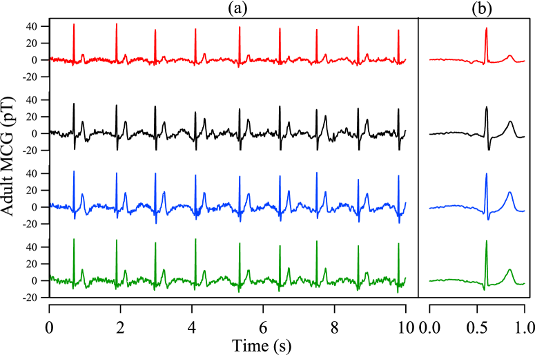
Figure 5: (a) Four-channel adult MCG with large signal interferences subtracted. (b) Shows the same set of MCG after averaging each channel.

We obtained MCG from 13 adult human subjects. The experimental protocol was approved by the institutional human subjects committee prior to commencement of the study and informed consent was obtained from all subjects.

Each measurement consists of a 30 s MCG recording from each magnetometer sampled with the same parameters described above. For data analysis, the magnetic field in the time-domain is obtained by a deconvolution of the magnetometer response (measured in the calibration) from the measured signal. The signal is then down-sampled to 1024 Hz. Low frequency drift is removed using a wavelet detrending algorithm.

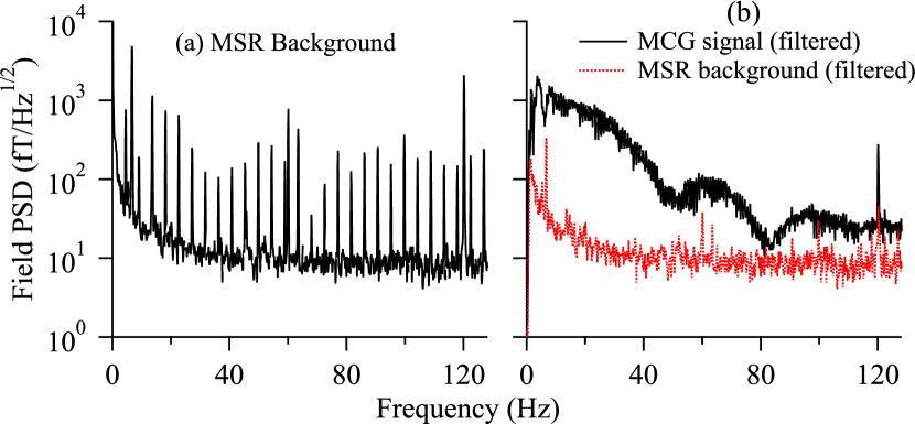
Figure 6: (a) MSR noise background for the MCG data. The peaks are actual magnetic artifacts, likely from building air-handling units, and comparison with figure 4, obtained on a different day, illustrates the day-to-day variation in the MSR background fields. (b) MCG signal (black) and MSR noise background (red dots) after the signal processing described in the text. The non-biomagnetic peaks in (a) are easily removed.

Figure 5(a) shows a processed segment of 30 s MCG recordings from the four channels. Figure 6(a) shows a reference measurement taken just after the data presented in figure 5, but without a subject. This measurement was taken on a different day than figure 4 and there are clearly more peaks, mostly at 4.55 Hz and its harmonics, along with a prominent 6.7 Hz peak and powerline harmonics. To obtain the traces in figure 5(a), the magnitude and phase of these non-biomagnetic peaks is determined from the reference, and then a matching sinusoid is subtracted from the signal channels, resulting in the PSDs shown in figure 6(b). Figure 5(b) shows the averaged traces. The P, QRS, and T components are well resolved. We emphasize these are magnetometer signals (rather than gradiometer signals), and contain any unfiltered background magnetic noise in the MSR as well as the MCG signal.

We estimate the minimum distance to the skin for each magnetometer of around 1 cm. ? reported their sensor head volume was located 5 mm from the skin or 5 cm from the heart, whereas the SQUIDS used for comparison were 7.5 cm from the heart. With our channel spacing (7 cm), we estimate each magnetometer is 7.6 cm from the heart when the array is centered above it.

Table 1: QRS peak amplitudes of this work. QRS dipole moments are estimated to compare with previous works. The distance range quoted here is for the range of individual magnetometer distances to the heart.

• 	(?)	(?)	This work
  $r$ (cm)	8–10.5	5	5.5–10.8
  $B_{\mathrm{QRS}}$ (pT)	(not reported)	100–150	$40\pm 16$
  $m$ ($\mathrm{\mu}$Am2)	0.76 $\pm 0.36$	0.4–0.6a	$0.60\pm 0.48^{\mathrm{a}}$

• ^a Estimated from $B_{\mathrm{QRS}}$ and $r$.

A statistical summary of the QRS peaks of 13 subjects is presented in table 1, along with an estimation of the QRS dipole amplitude $m$. We use the approximation $B_{\mathrm{QRS}}\sim m/r^{2.6}$ (?) to account for distributed source effects. To calculate $m$, we require the distance from the heart to each magnetometer. We minimize the standard deviation of $m$ across the four magnetometers as a function of the heart position with respect to the center of the magnetometer array, which can then be used to calculate the dipole amplitude for each patient. The result from this work in table 1 is a weighted mean of the 13 measured subjects.

In addition to adult MCG measurements, we also simulated MCG using a head phantom (Biomagnetic Technologies), which is a spherical shell filled with saline solution and five different current dipoles that can be driven individually. The head was placed as close as possible to the array centre and aligned so that the detected signal from driving a dipole was maximized. We drove the phantom with a test waveform (?) shown in figure 7(b).

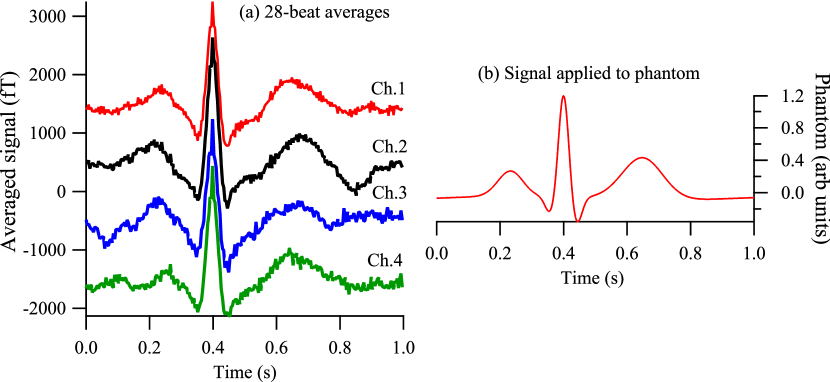
Figure 7: (a) 28-beat average response from the phantom driven with the waveform shown in (b), with magnetic field offsets applied to aid visualization. Before averaging, the signals are processed in the same way as the MCG above, by removing only narrow frequency components.

We used the calibrated magnetometers to adjust the QRS peak height driven by an amplitude scaled version of the test waveform. Figure 7(a) shows 28-beat averages for all four magnetometer channels, after processing the signals in the same way as the MCGs. The detected QRS amplitude is about 2 pT, and the averages for each channel faithfully represent the field expected from the driving waveform.

6 Noise sources and characterization

There are several different sources of unwanted signal in our magnetometer. These fall into three general categories. One is technical noise, including electrical pickup noise or probe movement on the detector photodiodes. The second is magnetic signal other than the desired biomagnetic signals, and the third noise category is fundamental quantum noise associated with the magnetic measurement. The last two terms are the dominant noise sources and we estimate the noise floor in table 2.

Table 2: Magnetometer Noise Budget. Two results are quoted for the photon shot noise. The basic model is (6) where $P_{z}$, $\Gamma_{\mathrm{pr}}$, and $\Gamma$ are all averages over the laser interaction volume. In the detailed model, these quantities are calculated at each position within the cell and then integrated to recover the photon shot noise floor.

• Noise Source	Level ( fT Hz-1/2)
  MSR Johnson noise	5
  Electrical current noise in nulling coils	3.9
  87Rb Johnson noise	0.9
  Photon shot noise (basic model)	0.3
  Photon shot noise (detailed model)	2
  Spin-projection noise	0.03
  Total	6.2

6.1 Magnetic noise

Magnetic noise generally includes any magnetic source that falls within the frequency band of interest and limits the achievable SNR of the desired signal. Clear examples can be seen in figure 6(a).

The single channel magnetometer noise floor in figure 4(b) and figure 6 is limited by Johnson noise in nearby electrical conductors. These conductors carry thermal currents which generate white-noise profile magnetic fields. The most important noise sources in our case are likely the mu-metal walls of the MSR and ⁸⁷Rb thin-film remaining on the Pyrex cell walls. We estimate these contributions from the calculations of ?. The 2 m cube shielded room has a noise floor of around 5 fT Hz^-1/2. We roughly model the ⁸⁷Rb film as a cylinder with a 1 cm radius and 10 nm thickness, about 5 mm from the detection volume, which would have a 0.9 fT Hz^-1/2 noise level.

We also measured the electrical current noise in the circuitry used to drive our nulling coils using a transimpedance amplifier. This contributes 3.9 fT Hz^-1/2 to the magnetic noise level.

6.2 Photon shot noise

Though most SERF magnetometers are limited by shield Johnson noise, there are two fundamental quantum noise sources which limit the maximum theoretical magnetic field resolution: spin-projection noise and photon shot noise. We briefly discuss the results in ? as they pertain here to photon shot noise. We estimate spin-projection noise to be a negligible contribution to the overall noise budget.

Photon shot noise occurs because the polarisation of the probe laser is determined by counting the difference in the number of photons arriving at the two different photodiodes in figure 1(a). The resulting uncertainty in the magnetic field is

$$\delta\Omega_{y}=\frac{2\Gamma}{P_{z}\sqrt{\Gamma_{\mathrm{pr}}\mathrm{OD}_{0}nVt}},$$ (6)

where $\mathrm{OD}_{0}=2r_{\mathrm{e}}fcnl/\Delta\gamma$ is the probe optical depth on resonance.

The parameters used in our calculations were $R=2575$/s, $\Gamma_{\mathrm{sd}}=60$/s, $\Gamma_{\mathrm{pr}}=155$/s, $n=7.8\times 10^{13}$/cm³, pump waist $w_{0,\mathrm{pu}}=2.6$ mm, and probe waist $w_{0,\mathrm{pr}}=1.1$ mm, and interaction volume $V=\pi w_{0,\mathrm{pr}}^{2}2w_{0,\mathrm{pu}}$. Equation (6) estimates a photon shot noise level of 0.3 fT Hz^-1/2.

We have found using this calculation with spatially averaged laser parameters estimates a lower photon shot noise limited sensitivity than we actually achieve in our experiments. A more detailed (?) model approximating the pump and probe laser propagation through the cell and their Gaussian spatial profiles, gives a more realistic 2 fT Hz^-1/2.

For comparison, an experimental measure of the photon shot noise can be obtained using the measured differential photocurrent per unit field $\Delta I_{p}/\Delta B$ and an effective photocurrent shot noise where $I_{p}$ is the photocurrent from a single photodiode. The photon quantization noise is $\delta I_{p}/\sqrt{\textnormal{Hz}}=\sqrt{2eI_{p}}$. The effective magnetic field noise is then

$$\frac{\delta B}{\sqrt{\textnormal{Hz}}}=\frac{\delta I_{p}/\sqrt{\textnormal{Hz}}}{\Delta I_{p}/\Delta B}.$$ (7)

For a typical measured ${\Delta I_{p}/\Delta B}=8$ $\mathrm{\mu A}/\mathrm{nT}$ operating with all four channels and a total probe power of 1.67 mW, $\delta B/\sqrt{\textnormal{Hz}}=$ 1.4 fT Hz^-1/2 from (7), in reasonable agreement with the more detailed calculation.

7 Conclusions and future work

We have presented a modular four-channel atomic magnetometer array operating in the SERF regime. The adjustable 7 cm channel spacing used for these measurements is much larger than previously presented biomagnetic measurements using SERF magnetometers. The single channel sensitivity ranged from 6–11 fT Hz^-1/2, dominated by magnetic noise from the MSR. The modularity of the magnetometers, in principle, allows flexible channel positioning in an array, despite large light shifts in different directions in the room reference frame.

Our sensitivity is limited by real magnetic noise. In this case, parametric modulation (?) can allow simultaneous measurement of $B_{x}$ and $B_{y}$, at the cost of a small (1/2 – 1/4) decrease in signal size. Future work will aim at using parametric modulation to measure two components of the magnetic field with each modular unit.

Detection of fMCG, an application which requires high sensitivity but a modest number of channels, should be possible with our array. However, the number of channels is insufficient to allow the effective use of spatial filters, such as beamformers and independent component analysis, which are widely used to remove maternal interference and to improve the signal-to-noise ratio of fMCG recordings. With a modest reduction in size, the design can be extended to higher channel counts. This will be essential for constructing dense arrays suitable for MEG and adult MCG.

References

References

- [1]
- [2] [] Allred J C, Lyman R N, Kornack T W & Romalis M V 2002 Physical review letters 89(13), 130801.
- [3]
- [4] [] Anderson L, Pipkin F & Baird Jr J 1960 Physical Review 120(4), 1279.
- [5]
- [6] [] Appelt S, Baranga A B A, Young A & Happer W 1999 Physical Review A 59(3), 2078–2084.
- [7]
- [8] [] Bison G, Castagna N, Hofer A, Knowles P, Schenker J L, Kasprzak M, Saudan H & Weis A 2009 Applied Physics Letters 95(17), 173701–173703.
- [9]
- [10] [] Bork J, Hahlbohm H, Klein R & Schnabel A 2000 in ‘Biomag’ pp. 970–973.
- [11]
- [12] [] Budker D & Romalis M V 2007 Nature Physics 3(4), 227–234.
- [13]
- [14] [] Cohen D, Edelsack E A & Zimmerman J 1970 Applied Physics Letters 16(7), 278.
- [15]
- [16] [] Cuneo B F, Ovadia M, Strasburger J F, Zhao H, Petropulos T, Schneider J & Wakai R T 2003 The American journal of cardiology 91(11), 1395–8.
- [17]
- [18] [] Dang H B, Maloof A C & Romalis M V 2010 Applied Physics Letters 97(15), 151110.
- [19]
- [20] [] Goldberger A, Amaral L, Glass L, Hausdorff J, Ivanov P, Mark R, Mietus J, Moody G, Peng C & Stanley H 2000 Circulation 101(23), e215.
- [21]
- [22] [] Hämäläinen M, Hari R, Ilmoniemi R J, Knuutila J & Lounasmaa O V 1993 Reviews of Modern Physics 65(2), 413–497.
- [23]
- [24] [] Happer W 1972 Reviews of Modern Physics 44(2), 169–249.
- [25]
- [26] [] Happer W & Tang H 1973 Physical Review Letters 31(5), 273–276.
- [27]
- [28] [] Johnson C N, Schwindt P & Weisend M 2010 Applied Physics Letters 97(24), 243703.
- [29]
- [30] [] Knappe S, Sander T H, Kosch O, Wiekhorst F, Kitching J & Trahms L 2010 Applied Physics Letters 97(13), 133703.
- [31]
- [32] [] Ledbetter M P, Savukov I M, Acosta V M, Budker D & Romalis M V 2008 Physical Review A 77(33408), 33408.
- [33]
- [34] [] Lee S K & Romalis M V 2008 Journal of Applied Physics 103, 84904.
- [35]
- [36] [] Li Z 2006 Development of a Parametrically Modulated SERF Magnetometer PhD thesis University of Wisconsin-Madison.
- [37]
- [38] [] Li Z, Wakai R T, Paulson D N & Schwartz B 2004 Neurology & clinical neurophysiology : NCN 2004, 25.
- [39]
- [40] [] Li Z, Wakai R T & Walker T 2006 Applied Physics Letters 89, 134105.
- [41]
- [42] [] Nousiainen J, Oja S & Malmivuo J 1994 Journal of electrocardiology 27(3), 221–231.
- [43]
- [44] [] Robbes D 2006 Sensors and Actuators A: Physical 129(1-2), 86–93.
- [45]
- [46] [] Savukov I M & Romalis M V 2005 Physical Review A 71(2), 23405.
- [47]
- [48] [] Seltzer S & Romalis M V 2004 Applied physics letters 85, 4804.
- [49]
- [50] [] Shah V, Knappe S, Schwindt P & Kitching J 2007 Nature Photonics 1(11), 649–652.
- [51]
- [52] [] Wakai R T, Lengle J M & Leuthold A C 2000 Physics in medicine and biology 45(7), 1989–95.
- [53]
- [54] [] Wakai R T, Strasburger J F, Li Z, Deal B J & Gotteiner N L 2003 Circulation 107(2), 307–12.
- [55]
- [56] [] Walker T & Happer W 1997 Reviews of Modern Physics 69(2), 629–642.
- [57]
- [58] [] Walters L 1970 Journal of the American Ceramic Society 53(5), 288–288.
- [59]
- [60] [] Xia H, Baranga A B A, Hoffman D & Romalis M V 2006 Applied Physics Letters 89, 211104.
- [61]