Formalising the Continuous/Discrete Modeling Step

Abstract

Formally capturing the transition from a continuous model to a discrete model is investigated using model based refinement techniques. A very simple model for stopping (eg. of a train) is developed in both the continuous and discrete domains. The difference between the two is quantified using generic results from ODE theory, and these estimates can be compared with the exact solutions. Such results do not fit well into a conventional model based refinement framework; however they can be accommodated into a model based retrenchment. The retrenchment is described, and the way it can interface to refinement development on both the continuous and discrete sides is outlined. The approach is compared to what can be achieved using hybrid systems techniques.

1 Introduction

Conventional model based formal refinement technologies (see for example [38, 20, 39, 2, 35, 44, 3]) are based on purely discrete mathematical and logical concepts. These turn out to be ill suited to modeling and formally developing applications whose usual models are best expressed using continuous mathematics. Nevertheless, many such applications, control systems in particular, are these days implemented using digital techniques. So there is a mismatch between continuous modeling and discrete development techniques.

In this paper we tackle this mismatch head on. Although traditional model based refinement is too exacting to straddle the continuous to discrete demarcation line, a judicious weakening of it, retrenchment, proves to be adaptable enough to do the job, which we show. Importantly, retrenchment techniques interface well with refinement, so that a development starting from continuous and ending at discrete can be captured in an integrated way.

In this paper we tackle the continuous to discrete issue by taking a simple running example, one that can be solved fully by analytic means in both the continuous and discrete domains, and tracing it through the critical formal development step. We start with a continuous control problem: bringing an object (eg. a train) to a halt. This is formulated as a continuous control problem, and given the (deliberately chosen) simplicity of the problem, an exact solution is presented. In reality, continuous control is implemented these days via digital controllers. These periodically read inputs and recompute outputs at multiples of a sampling interval during the dynamics. In this sense, the control becomes discretized, although the discretized control is obviously still played out in the continuous real world. We thus remodel the continuous problem as a discrete control problem, and derive a formal description of the discretization step via a suitable retrenchment, drawing on rigorous results from the theory of ordinary differential equations (ODEs) to supply the justification. Given the limited size of this paper, our technical focus is on this critical step, and the remainder of the development (comprising the associated refinements either side of it) is sketched rather than treated in detail. The latter is a task for which a fuller treatment will be given in the extended version of the paper.

The rest of the paper is as follows. We start in Section 2 by describing relevant existing work in the hybrid systems domain and how it contrasts with our own approach, after which we get down to details. Section 3 then formulates our train stopping problem as a conventional open loop continuous control problem. Section 4 then describes the discretization of the control problem using a simple zero order hold strategy. In Section 5 we review what we need of ASM refinement and retrenchment in a form suitable for our problem. Section 6 then shows how our earlier discretization process can be captured using a suitable retrenchment, citing the needed ODE results. Section 7 sketches how all this can fit into a wider formal development strategy, in which the greater flexibility of retrenchment can be combined with the stronger guarantees offered by refinement via the Tower Pattern [9, 29]. Section 8 concludes.

2 Related Work

The relationship between continuous and discrete transition systems has long been a topic for investigation in the hybrid systems field. Earlier work includes [5, 27, 6, 26]; also, the International Conference on Hybrid Systems: Computation and Control, has been the venue for a large amount of research in this area. A more recent reference is [43].

Hybrid systems are dynamical systems that mix smooth, continuous transitions with discrete, discontinuous ones. The major focus in this field has been the automatic verification of properties of such systems. Obviously, such verification demands the representation of the systems in question in discrete and finite terms, whether by means of an explicitly constructed finite state space (which is manipulated directly), or a state space whose states arise via the symbolic representation of the less tractable state space of a previously constructed underlying system (which is manipulated symbolically).

The main tool for bringing an intractable state space within the scope of computable techniques is the equivalence relation. Regions of the state space are gathered into equivalence classes, and a representation of these equivalence classes (whether as individual elements in a simple approach, or as symbolic expressions that denote the equivalence class in question) constitutes the state space of the abstraction. Transitions between these states are introduced to mirror the behaviour of the underlying system. The properties of interest can then be checked against the abstract system. For instance, properties that can be expressed as reachability properties fall within the scope of model checking approaches that are applied to the abstraction.

Of course what has been constructed thereby is a (bi)simulation, and a major strand of hybrid systems research is the investigation of such (bi)simulations. The same remarks apply when there is an external control applied to the systems.

One disadvantage of the above approach is the frequent reliance on brittle properties of the studied systems. Put most simply, a number of techniques rely on the parameters of the problem falling within a subset of measure zero of the parameter space. Real systems can never hit such small targets reliably. Equally, the simulation relations studied can also be just as brittle. To alleviate this, and to address other issues of interest, the notion of approximate (bi)simulation has been studied in recent years ([43] gives a good introduction). Here, instead of defining the simulation relation $R(u,v)$ between an abstract state $u$ and a concrete state $v$ as a simple predicate on states, it is defined via a distance function $\mathbf{d}$ as $R_{\epsilon}(u,v)\equiv\mathbf{d}(f(u),v)\leq\epsilon$, where $f$ is a precise relationship between the two state spaces which is in some sense “semantically natural” (we don’t have space to elaborate on this aspect here). For bisimulation you need a symmetrical arrangement of course.

(Bi)simulation depends on assuming the appropriate relation between the two before-states and re-establishing it in the after-states of suitable pairs of transitions. To preserve a relationship based on distance, the dynamics needs to be inherently stable. The obvious centre of attention thus becomes stable control systems, normally linear stable control systems, because of their calculational tractability. These are discussed in very many places, eg. [33, 21, 23, 19, 4, 41, 12, 7].

In a stable system all trajectories converge to a single point, so the distance between two trajectories decreases monotonically; hence a simulation relation based on distance between trajectories is maintained. But although most systems are designed to be stable in this sense, some are not, and there can be parts of a system phase space in which trajectories diverge rather than converge, without rendering the system useless. Below, we treat in detail a very simple example which happens to be unstable in the sense just discussed. We know it is not stable because we solve it exactly.

Also, in the usual hybrid systems literature, it is normal that the discrete approximation to a given system is manufatured from it (eg. by constructing equivalence classes, as indicated above). In our approach, by contrast, we take a more “off the shelf” attitude to discretization, analysing a straightforward “zero order hold” version of the continuous system (in which the new output values to be sent to the actuators are recalculated at regular intervals, and the new values are “held” for the duration of the next inteval) rather than something extracted from an analysis of the original system. In this sense our approach is closer to conventional engineering practice, since it is directed at the typical practical approach. Of course these two ways of doing things are not mutually exclusive: the parameters of the zero order hold may fall within the parameters of a discrete approximation extracted by analysis of the original system, and vice versa. Finally, our approach is via retrenchment, one consequence of which is that our analysis is not confined to the purely stable case. In effect, the greater expressiveness of retrenchment permits (the analogue of) the simulation relation mentioned above, to increase its permitted margin of error, as well as to decrease it, although this emerges indirectly.

3 Train Stopping: a Continuous Control System

Our target application domain is control problems in the railway sphere. In this paper we have train stopping as a specific case study. Of course, in reality, train position control is a complex problem [42, 28], relying on the co-operation of many mechanisms to achieve a reliable outcome, and we do not have the space to deal with all these aspects and their subtle interactions. Instead we focus on a single technical issue —the relationship between a continuous control problem and its discrete counterpart— in a very simple way, commenting on the extreme simplicity below.

Suppose a train, of mass $M$, is traveling at its cruise velocity $V$, when it needs to stop. We assume that a linearly increasing deceleration rate $a$ is appropriate. (It has to be said here that our notion of appropriateness is not quite the usual one. Rather than usability or any similar consideration governing our choice, simplicity is the priority. A constant deceleration would have been even simpler — unfortunately the zero order hold approximation to constant deceleration is identical to it, trivialising our problem.) To bring the train to a standstill using linearly increasing deceleration, a force $F=-Mat$ (where $t$ is time) has to be applied, by Newton’s Law. We will assume that $M$ is known, so that we can focus on just the kinematic aspects.

A cursory knowledge of kinematics is enough to reveal that under linear deceleration, the deceleration, distance and stopping time are linked. We suppose that there is a single stopping episode, which starts at time $0$ and at $x$ position $0$, and which ends at time $T_{Stop}$, with the train having traveled to position $x=D$. Representing time derivatives with a dot, if $v$ is the velocity, then we know that

$$\dot{v} ~{}=~{}-at v(0) ~{}=~{}V v(T_{Stop}) ~{}=~{}0$$ (1)

Regarding the distance traveled $x$, we know that

$$\dot{x} ~{}=~{}v x(0) ~{}=~{}0 x(T_{Stop}) ~{}=~{}D$$ (2)

Integrating these, rapidly brings us to

$$V ~{}=~{}\frac{1}{2}aT_{Stop}^{2} D ~{}=~{}VT_{Stop}-\frac{1}{3!}aT_{Stop}^{3}~{}=~{}\frac{2}{3}VT_{Stop}$$ (3)

We now recast the above as a control theory problem. At the introductory level, control theory is usually developed in the frequency domain [33, 21, 23, 19], because of the relative simplicity and perspicuity of the design techniques in that domain. However, for results sufficiently rigorous to interface to formal techniques, we need to go to the state space formulation favoured by more mathematically precise treatments [4, 41, 16, 15, 12, 7]. In the state space picture, the system consists of a number of state variables, and their evolution is governed by a corresponding number of first order differential equations. State variables and differential equations mirror the states and transition systems of model based refinement formalisms sufficiently closely that we can hope to make a connection between them.

To use the first order framework in our example, the state has to consist of both the position $x(t)$ and the velocity $v(t)$. So we get the state vector

$$\boldsymbol{x}(t)~{}=~{}\begin{bmatrix}x(t)\\ v(t)\end{bmatrix}$$ (4)

The dynamics of the system is captured in the equation

$$\dot{\boldsymbol{x}}(t)~{}=~{}\begin{bmatrix}\dot{x}(t)\\ \dot{v}(t)\end{bmatrix}~{}=~{}\boldsymbol{f}(\dot{x}(t),u(t))~{}=~{}\begin{bmatrix}v(t)\\ u(t)\end{bmatrix}$$ (5)

where

$$u(t)~{}=~{}-at$$ (6)

is the external control control signal. We also have the initial condition

$$\boldsymbol{x}(0)~{}=~{}\begin{bmatrix}0\\ V\end{bmatrix}$$ (7)

4 From Continuous Control to Discrete Control

To truly implement a continuous control model, such as our case study, requires analogue apparatus. In the highly digitized world of today, hardly any such systems are built. Instead, continuous control designs are discretized, and it is the corresponding digital control systems that are implemented.

The digital approach to control has many parallels with the continuous case — in the frequency domain the main difference is the use of the $z$-transform rather than the Laplace transform. The state based picture too boasts many parallels, with first order difference equations replacing first order differential equations [24, 25, 34, 30].

In this section we examine a discrete counterpart of the previous continuous control problem, in preparation for a formal reappraisal in the next section. One advantage of the extreme simplicity of our example, is that it admits an analytic solution in both continuous and discrete domains, enabling an incisive evaluation to be made later, of the reappraisal in Section 6.3.

The starting point for our problem remains as before: the train, traveling at velocity $V$, needs to stop after time $T_{Stop}$, having gone a distance $D_{D}$. Instead of doing so continuously though, it will do it in a number of discrete episodes. For this purpose, let us assume that $T_{Stop}$ is divided into $N$ short periods, each of length $T$, so that

$$T_{Stop}~{}=~{}NT$$ (8)

Our discretization scheme will be based on a zero order hold, in which the same control input value is maintained throughout an individual time period. The counterpart of the linear deceleration rate $a$ of the continuous treatment, will be a piecewise constant deceleration, with the constant rate decreasing by an additional multiple of a constant $a_{D}$ after each time interval of length $T$.

Calling the discretized velocity variable $v_{D}$, we have for the acceleration

$$\dot{v}_{D}(t)~{}=~{}-ka_{D}T$$ (9)

where

$$k~{}=~{}\left\lceil\frac{t}{T}\right\rceil$$ (10)

and $k$ ranges over the values $1\ldots N$. If we set, for a general $t$,

$$\delta t_{k}~{}=~{}t-(k-1)T~{}=~{}t-\left\lfloor\frac{t}{T}\right\rfloor T$$ (11)

then recalling that the initial velocity is $V$, provided $(k-1)T<t<kT$, the velocity during the $k$’th period is

$$v_{D}(t)~{}=~{}V-a_{D}T^{2}-2a_{D}T^{2}-\ldots-(k-1)a_{D}T^{2}-ka_{D}T\delta t_{k}$$ (12)

Since the final velocity is zero, we derive

$$V~{}=~{}a_{D}T^{2}+2a_{D}T^{2}+\ldots+Na_{D}T^{2}~{}=~{}\frac{1}{2}a_{D}T^{2}N(N+1)$$ (13)

Knowing the velocity, we can integrate again, and work out the distance traveled. Calling the displacement in the discretized world $x_{D}$, the contribution to $x_{D}$ during the period $(k-1)T<t<kT$ comes out as

$$(V-a_{D}T^{2}-2a_{D}T^{2}-\ldots-(k-1)a_{D}T^{2})\delta t_{k}-\frac{1}{2}ka_{D}T\delta t_{k}^{2}$$ (14)

Thus for the total distance we find

$$D_{D} ~{}=~{}NVT-a_{D}T^{3}\sum^{N-1}_{k=1}(N-k)k-\frac{1}{2}a_{D}T^{3}\sum^{N}_{k=1}k$$

$$~{}=~{}VT_{Stop}-\frac{1}{12}a_{D}T^{3}(2N^{3}+3N^{2}+N)$$ (15)

Both (13) and (15) feature $a_{D}$. Substituting the $a_{D}$ value from (13) into (15) gives

$$D_{D} ~{}=~{}VT_{Stop}\left[1-\frac{2N^{2}+3N+1}{6N^{2}+6N}\right]~{}=~{}\frac{2}{3}VT_{Stop}\left[1-\frac{1}{4N}+O(N^{-2})\right]$$ (16)

We see that (16) for $D_{D}$ contains an $O(1/N)$ correction compared with (3) for $D$ (assuming we keep $V$ and $T_{Stop}$ the same). This is because we have an extra constraint generated by the requirement that $T_{Stop}$ is an integral multiple of $T$, making the problem overconstrained if we wished $D$ and $D_{D}$ to be the same.

Recasting the preceding as an initial value first order system along the lines of (4)-(7) is not hard. The state vector is

$$\boldsymbol{x}_{D}(t)~{}=~{}\begin{bmatrix}x_{D}(t)\\ v_{D}(t)\end{bmatrix}$$ (17)

and the dynamics of the system is captured in the equation

$$\dot{\boldsymbol{x}}_{D}(t)~{}=~{}\begin{bmatrix}\dot{x}_{D}(t)\\ \dot{v}_{D}(t)\end{bmatrix}~{}=~{}\boldsymbol{f}(\dot{x}_{D}(t),u_{D}(t))~{}=~{}\begin{bmatrix}v_{D}(t)\\ u_{D}(t)\end{bmatrix}$$ (18)

where

$$u_{D}(t)~{}=~{}\dot{v}_{D}(t)~{}=~{}-ka_{D}T$$ (19)

as given by (9), is the external control. We also have the initial condition

$$\boldsymbol{x}_{D}(0)~{}=~{}\begin{bmatrix}0\\ V\end{bmatrix}$$ (20)

It is hard not to notice how much more complicated the above is compared with (1)-(7). It is always so with discrete systems — hence the strong desire to model systems in the continuous domain. The very rapid ramp-up in complexity when we consider the discrete version of a continuous problem is our justification for restricting to a particularly simple example. The ability to keep the complexity still low enough to permit an exact solution, is extremely useful in an investigation such as this one, allowing a comparison between exact and approximate approaches to be made with confidence.

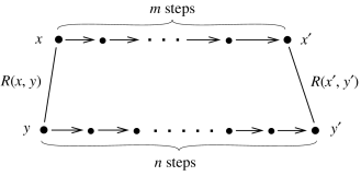
Figure 1: An ASM $(m,n)$ diagram, showing how $m$ abstract steps, going from state $x$ to state $x^{\prime}$ simulate $n$ concrete steps, going from $y$ to $y^{\prime}$. The simulation is embodied in the retrieve relation $R$, which holds for the before-states of the series of steps $R(x,y)$, and is re-established for the after-states of the series $R(x^{\prime},y^{\prime})$.

5 ASM Refinement and Retrenchment

In this section we review what we need of ASM refinement and retrenchment, which will be the vehicles for formalization in this paper. The standard reference for the ASM method is [14], building on the earlier [13]. In general, to prove an ASM refinement, one verifies so-called $(m,n)$ diagrams, in which $m$ abstract steps simulate $n$ concrete ones. The situation is illustrated in Fig. 1, in whch we suppress input and output for clarity. For this paper, it will be sufficient to focus on the refinement proof obligations (POs) which are the embodiment of this policy. The first is the initialization PO:

$$\forall\,y^{\prime}\bullet CInit(y^{\prime})\Rightarrow(\exists\,x^{\prime}\bullet AInit(x^{\prime})\land R(x^{\prime},y^{\prime}))$$ (21)

In (21), it is demanded that for each concrete initial state $y^{\prime}$, there is an abstract initial state $x^{\prime}$ such that the retrieve or abstraction relation $R(x^{\prime},y^{\prime})$ holds.

The second PO is correctness, and is concerned with the verification of the $(m,n)$ diagrams. For this, we have to have some way of deciding which $(m,n)$ diagrams are sufficient for the application. Let us assume that we have done this. Let $CFrags$ be the set of fragments of concrete execution sequences that we have previously determined will permit a covering of all the concrete execution sequences of interest for the application. We write $y::ys::y^{\prime}\in CFrags$ to denote an element of $CFrags$ starting with concrete state $y$, ending with concrete state $y^{\prime}$, and with intervening concrete state sequence $ys$. Likewise $x::xs::x^{\prime}\in AFrags$ for abstract fragments. Also, let $is,js,os,ps$ denote the sequences of abstract inputs, concrete inputs, abstract outputs, concrete outputs, respectively, belonging to $x::xs::x^{\prime}$ and $y::ys::y^{\prime}$, and let $In(is,js)$ and $Out(os,ps)$ denote suitable input and output relations. Then the correctness PO reads:

$$\forall\,x,is,y,ys,y^{\prime},js,ps\bullet y::ys::y^{\prime}\in CFrags\land R(x,y)\land In_{AOps,COps}(is,js)~{}\land$$

$$\quad COps(y::ys::y^{\prime},js,ps)$$

$$\qquad\Rightarrow(\exists\,xs,x^{\prime},os\bullet AOps(x::xs::x^{\prime},is,os)\land R(x^{\prime},y^{\prime})\land Out_{AOps,COps}(os,ps))$$ (22)

In (22), it is demanded that when there is a concrete execution fragment of the form $COps(y::ys::y^{\prime},js,ps)$, carried out by a sequence of concrete operations $COps$, with state sequence $y::ys::y^{\prime}$, input sequence $js$ and output sequence $ps$, such that the retrieve and input relations $R(x,y)\land In(is,js)$ hold between concrete and abstract before-states and inputs, then an abstract execution fragment $AOps(x::xs::x^{\prime},is,os)$ can be found to re-establish the retrieve and output relations $R(x^{\prime},y^{\prime})\land Out(os,ps)$.

The ASM refinement policy also demands that non-termination be preserved from concrete to abstract, but we will not need that in this paper. We now turn to retrenchment.

For retrenchment, [11, 10] give definitive accounts; latest developments are found in [37]. See also [8] for formulations of retrenchment adapted to several specific model based refinement formalisms including ASM. Like refinement, retrenchment is also characterized by POs: an initialization PO identical to (21), and a “correctness” PO which weakens (22) by inserting within, output and concedes relations, $W_{Op},O_{Op},C_{Op}$ respectively into (22), to give extra flexibility and expressivity. In particular, the concession $C_{Op}$ weakens the conclusions of (22) disjunctively, giving room for many kinds of “exceptional” behaviour. The result is:

$$\forall\,x,is,y,ys,y^{\prime},js,ps\bullet y::ys::y^{\prime}\in CFrags\land R(x,y)\land W_{AOps,COps}(is,js,x,y)~{}\land$$

$$\quad COps(y::ys::y^{\prime},js,ps)$$

$$\qquad\Rightarrow(\exists\,xs,x^{\prime},os\bullet AOps(x::xs::x^{\prime},is,os)~{}\land$$

$$\qquad\qquad\qquad\quad((R(x^{\prime},y^{\prime})\land O_{AOps,COps}(x::xs::x^{\prime},is,os,y::ys::y^{\prime},js,ps))~{}\lor$$

$$\qquad\qquad\qquad\quad~{}~{}~{}C_{AOps,COps}(x::xs::x^{\prime},is,os,y::ys::y^{\prime},js,ps)))$$ (23)

To ensure that retrenchment only deals with well defined transitions, and to ensure smooth retrenchment/refinement interworking, we also insist that $R\land W_{Op}$ always falls in the domain of the requisite operations, though this is another thing not needed here.

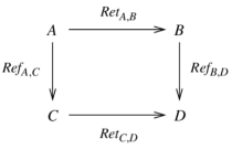
Figure 2: The Tower Pattern basic square, with refinements vertical, retrenchments horizontal.

The smooth interworking between refinements and retrenchments is guaranteed by the Tower Pattern. The basic construction for this is shown in Fig. 2. There, refinements are vertical arrows and retrenchments are horizontal, and the two paths round the square from $A$ to $D$ (given by composing $Ref_{A,C}$ with $Ret_{C,D}$ on the one hand, and on the other, by composing $Ret_{A,B}$ with $Ref_{B,D}$) are compatible, in the sense that they each define a portion of a (potentially larger) retrenchment from $A$ to $D$.

At this point one might legitimately ask what all the above has to do with our case study, in which the dynamics that we considered is entirely in the continuous domain (albeit taking into account discontinuous control inputs when necessary). The answer lies in the focus on the use of paths through the system at both abstract and concrete levels in the POs of ASM. With this focus, it is unproblematic to reconfigure the $(m,n)$ rules (22) and (23) to deal with continuous paths rather than discrete ones. Thus $CFrags$ and $AFrags$ can now refer to fragements of continuous system trajectories, rather than sequences of state-to-state hops. Likewise the $is$ and $js$ in $W_{AOps,COps}(is,js,x,y)$ now refer to the continuous input signals along the trajectories, and so on for the other terms in (22) and (23). We see this exemplified in detail in the retrenchment of Section 6.2.

6 Formalizing the Continuous to Discrete Modeling Change

In the control literature, one finds many ways of discretizing continuous designs (see loc. cit.), and the evaluation of the relationship between continuous and discrete is often based on ad hoc engineering rules of thumb. While these typically yield perfectly good results in practice, the criteria used fall far short of the kind of precision needed for a good fit with model based formal development techniques. As a consequence, when model based formal development techniques are used to support the digital implementation of the discrete counterpart of some continuous design, the formal modeling inevitably starts already in the discrete domain. Obviously this yields a weaker formal support for the process than if the formal modeling had started earlier, at the continuous design stage, and was integrated into all the subsequent design steps, including the change from continuous to discrete.

Our objective in this paper is to illustrate how to make a judgement about the discretization of a control problem, that has enough precision to integrate well with model based formal technologies. To achieve this we have recourse to the rigorous theory of ODEs. It can be shown that two instances of a control problem which differ solely in the input control satisfy an inequality:

$$||\boldsymbol{x}^{u}-\boldsymbol{x}_{D}^{u_{D}}|| ~{}\leq~{}K\!\mathit{2}||u-u_{D}||_{2}$$ (24)

In (24), $||\boldsymbol{x}^{u}-\boldsymbol{x}_{D}^{u_{D}}||$ is the $\mathcal{L}^{\infty}$ norm of $\boldsymbol{x}^{u}-\boldsymbol{x}_{D}^{u_{D}}$, or, in plain English, the maximum value over the interval $[0\ldots T_{Stop}]$ attained by the difference between continuous and discrete values of any state component. Likewise, $||u-u_{D}||_{2}$ is the $\mathcal{L}^{2}$ norm of $u-u_{D}$, or, in plain English, the root integrated square difference between $u$ and $u_{D}$, calculated over the interval $[0\ldots T_{Stop}]$. Finally, $K\!\mathit{2}$ is a constant.

We note that the continuous and discrete versions of our case study, with initial states (7) and (20), over the time interval from $0$ to $T_{Stop}$, characterize just such a scenario, since (5) and (7) differ from (18) and (20) only in the use of $u_{D}$ rather than $u$ among the independent variables.

6.1 Rigorous Bounds on Continuous and Discrete Systems

We now flesh out what (24) means for our little case study. We consider the values of the quantities on the right hand side of (24) in order to obtain a bound for the value of the left hand side. Referring to (24), theory furnishes an explicit value for the constant $K\!\mathit{2}$, namely

$$K\!\mathit{2} ~{}=~{}e^{K_{\boldsymbol{f}}}||k_{u}||_{2}$$ (25)

In (25) $K_{f}$ is $k_{f}\,T_{Stop}$, where $k_{f}$ is the $\mathcal{L}^{\infty}$ norm of $\boldsymbol{f}_{\boldsymbol{x}}$, or, the absolute maximum value (over the interval $[0\ldots T_{Stop}]$) of the Lipschitz constant governing the variation of the control law $\boldsymbol{f}$ with respect to the state. In our application, the form of the control law is

$$\boldsymbol{f}(v(t),u(t))~{}=~{}\begin{bmatrix}v(t)\\ u(t)\end{bmatrix}$$ (26)

and it is clear that there is only one component of $\boldsymbol{f}$ with a non-zero partial derivative with respect to either $x$ or $v$, namely the first

$$\frac{\partial\boldsymbol{f}_{1}}{\partial v}~{}=~{}1$$ (27)

With this, the first factor of (25) is just $e^{T_{Stop}}$.

Regarding the second factor, $||k_{u}||_{2}$ is the root integrated square value of the Lipschitz constant governing the variation of the control law with respect to the input control signal. Again there is only one component of $\boldsymbol{f}$ with a non-zero partial derivative with respect to $u$, namely the second

$$\frac{\partial\boldsymbol{f}_{2}}{\partial u}~{}=~{}1$$ (28)

so the root integrated square reduces to $\sqrt{T_{Stop}}$. So we get

$$K\!\mathit{2} ~{}=~{}e^{T_{Stop}}\sqrt{T_{Stop}}$$ (29)

Turning to the second factor on the right hand side of (24), $||u-u_{D}||_{2}$, we recall that we know explicitly what $u$ and $u_{D}$ are from our earlier calculations. From (6) and (19) we know that

$$u(t) ~{}=~{}-at u_{D}(t)~{}=~{}-ka_{D}T$$ (30)

where, from (3) and (13)

$$a ~{}=~{}\frac{2V}{T_{Stop}^{2}} a_{D} ~{}=~{}\frac{2V}{T_{Stop}^{2}(1+1/N)}$$ (31)

Now (30) shows that $u(t)$ decreases linearly, and that $u_{D}(t)$ is a staircase function, decreasing in equal sized steps near $u(t)$. It is clear from (30) that in the limit $t\rightarrow 0+$, we have $u(0+)=0$ and $u_{D}(0+)=-a_{D}T$, so that $u(0+)-u_{D}(0+)=a_{D}T$. It is also clear from (30) that in the limit $t\rightarrow T_{Stop}-$, we have $u(T_{Stop}-)=-aT_{Stop}$ and $u_{D}(T_{Stop}-)=-Na_{D}T=-a_{D}T_{Stop}$, so that $u(T_{Stop}-)-u_{D}(T_{Stop}-)=(a_{D}-a)T_{Stop}=a_{D}T_{Stop}[1-(1+1/N)]=-a_{D}T_{Stop}/N=-a_{D}T$. Since the staircase has equal sized steps, it evidently the case that the staircase $u_{D}(t)$ ranges around $u(t)$ within a bound $a_{D}T$.

$$|u(t)-u_{D}(t)|~{}\leq~{}a_{D}T$$ (32)

This furnishes a suitable overestimate for the root integrated square difference between $u(t)$ and $u_{D}(t)$ as follows

$$||u-u_{D}||_{2}~{}\leq~{}\sqrt{\int_{t=0}^{T_{Stop}}[a_{D}T]^{2}dt}~{}=~{}a_{D}T\sqrt{T_{Stop}}$$ (33)

Substituting all the values we have obtained into (24), we get

$$||\boldsymbol{x}^{u}-\boldsymbol{x}_{D}^{u_{D}}||~{}\leq~{}e^{T_{Stop}}\sqrt{T_{Stop}}\times a_{D}T\sqrt{T_{Stop}}~{}=~{}e^{T_{Stop}}a_{D}TT_{Stop}$$ (34)

We see that despite the potential for the deviation between $u(t)$ and $u_{D}(T)$ to grow exponentially with the size of the time interval, a possibility severely exacerbated by our rather crude bound (33), it is always possible to reduce it by an arbitrary amount by making the discretization, measured by $N$, fine enough.

6.2 Turning Rigorous Bounds into Retrenchment Data

Now that we have a precise relationship between the continuous and discrete control systems, we can look to incorporate this into our model based formal description.

In general, the exigencies of model based formal refinement are too exacting to be able to accommodate the kind of relationships just derived. Retrenchment though, has been purposely designed to be more forgiving in this regard, so that is what we will use.

Regardless though, of which model based formal description technique is adopted, is the issue that all such techniques are designed for discrete state transitions, and presume a well defined notion of “next state”, to which an equally clear notion of “current state” can be related.

In continuous dynamics there is no sensible notion of next state that we can immediately use. However, as we noted above, the $(m,n)$ diagram approach of ASM refinement makes clear that it is paths at abstract and concrete levels that are being related. Thus, although we avoid technical details in this paper, we extend the ASM approach to incorporate continuous paths as well as discrete ones. The incentive to do this was one strong reason for choosing ASMs in this work. (Note that this perspective on refinememt between paths is equally applicable to both the continuous and discretized versions of our control problem. In the continuous problem there is a single continuous path. In the discretized problem there are $N$ consecutive shorter continuous “zero order held” paths, interleaved, at the instants at $kT$, by the discrete recalculations of the output signal, thus constituting a path comprising both continuous and discrete components.)

Since the rigorous results we use concern the same starting state for the two systems, our formal statement is constrained to be an end-to-end one. It will express an end-to-end relationship between the smooth dynamics at the continuous level, and the discretized level’s dynamics (which is continuous too, though punctuated at every multiple of $T$ by a discontinuous change in the acceleration).

As we saw before, a retrenchment between two specific operation sequences consists of four things: a retrieve relation between the state spaces, a within relation for the before-states and inputs, an output relation for the after-states and outputs (and before-states and inputs too if necessary), and a concedes relation for the after-states and outputs (and before-states and inputs too if needed). In the relations below, we use some ad hoc notations whose meaning should be obvious from the preceding material.

Regarding the retrieve relation $R$, there is a very natural one that we might expect to use, namely the identity between state values in the continuous and discretized worlds. However, even though in our specific case study the two models start out in the same state thus making such a putative $R$ true in the hypothesis of the PO (23), in most cases, that assumption will not hold, and so we prefer to follow a more generic approach, which will be applicable in a wider set of scenarios. A second proposal for $R$ would see it express a margin of tolerance between the state values in the continuous and discretized worlds, as discussed in Section 2. This proposal would also work after a fashion, but such a proposal works best when the relationship between the two system states is stable throughout the dynamics — we have then a kind of refinement. In our case study, this assumption does not hold since the discrepancy between the two system states grows steadily through the dynamics.

To accomodate inconvenient situations such as these, retrenchment makes provisions for expressing the relationship (or just aspects of the relationship) between the states at the before- point of the transition being discussed in the within relation $W$ instead of (or in addition to) in $R$. Since the facts expressed in $W$ do not need to be re-established in the conclusion of the PO (23), this provides the most flexible way of incorporating appropriate facts about the systems’ before-states in the PO. With this strategy, a global retrieve relation is not appropriate, and we set $R$ to true

$$R(\langle x(t),v(t)\rangle,\langle x_{D}(t),v_{D}(t)\rangle)~{}\equiv~{}\textsf{true}$$ (35)

The job of expressing that the before-states are suitably matched in the PO, taking into account the input control signals throughout the interval of interest, is thus taken on by the within relation $W$

$$W(u(t\in[0\ldots T_{Stop}]),u_{D}([t\in 0\ldots T_{Stop}]),\langle x(0),v(0)\rangle,\langle x_{D}(0),v_{D}(0)\rangle)~{}\equiv~{}$$

$$\quad x(0)=x_{D}(0)\land v(0)=v_{D}(0)~{}~{}~{}~{}\land~{}~{}~{}~{}||u-u_{D}||_{2}\leq a_{D}T\sqrt{T_{Stop}}$$ (36)

Note that while $W$ relates just the continuous and discrete before-states, it also relates the whole of the continuous and discrete control inputs.

The output relation $O$ says what happens at the end of the period of interest. In our case, on the basis of the rather heavy calculations that came earlier, we can use $O$ to say that the after-states diverge by no more than the bound derived in (34)

$$O(\langle x(T_{Stop}),v(T_{Stop})\rangle,\langle x_{D}(T_{Stop}),v_{D}(T_{Stop})\rangle)~{}\equiv~{}$$

$$\quad|x(T_{Stop})-x_{D}(T_{Stop})|\leq e^{T_{Stop}}a_{D}TT_{Stop}~{}~{}~{}~{}\land~{}~{}~{}~{}|v(T_{Stop})-v_{D}(T_{Stop})|\leq e^{T_{Stop}}a_{D}TT_{Stop}$$ (37)

Note that although $O$ itself speaks explicitly only about the after-states that are attained by the two systems, the fact that we derived the properties of the after-states in question using an $\mathcal{L}^{\infty}$ analysis, means that the same bound holds throughout the interval of interest. The advantage of this formulation is that we automatically get a discreteness of the description in terms of before- and after- states, which will integrate neatly with discrete system reasoners (in the event that such modeling is eventually incorporated into mechanised tools), while yet providing guarantees that hold throughout the interval of interest.

Since our system is so simple, $O$ already captures all that we need to say, and the kind of exceptional behaviour that may need to be taken into account in more realistic engineering situations is not present. This is also connected wsiyth the fact that we have trivialised the retrieve relation. Accordingly we can set the concedes relation $C$ to false

$$C(\langle x(T_{Stop}),v(T_{Stop})\rangle,\langle x_{D}(T_{Stop}),v_{D}(T_{Stop})\rangle)~{}\equiv~{}\textsf{false}$$ (38)

With these data, the proof obligation (23) becomes provable on the basis of the results cited earlier, which establishes the formal connection between the continuous and discrete domains in a way that can be integrated with formal refinements on both the continuous and discrete sides.

Particularly noteworthy is the fact that the discrepancy between the states grows linearly with time; and that this is a property of the exact solutions and not just an artifact of some approximation scheme. If we tried to handle this in a pure refinement framework, using a retrieve relation $R$ to capture the relationship between states in the two models (regardless of whether $R$ was an exact, pointwise relationship, or an approximate one, analogous to the approximate simulation relations discussed in Section 2), then assuming such an $R$ for the before-states would not enable us to re-establish it for the after-states, and the correctness PO could not be proved. The greater flexibiity of retrenchment permits us to handle the before-states in the within relation and the after-states in the output relation, overcoming the problem.

6.3 Corroboration

In our case study, exact solvability of the control models in both continuous and discrete domains gives us additional and independent confirmation of the approach we are advocating in this paper.

Both continuous and discrete models “run” for the same amount of time, $T_{Stop}$, and the output relation (37) gives an estimate for the discrepancy between the continuous and discrete states reached in the two models after that time. The states themselves consist of two components, the displacements and the velocities.

Regarding the velocities, both models come to a standstill after exactly $T_{Stop}$. Consequently both $v(T_{Stop})$ and $v_{D}(T_{Stop})$ are zero, so that $|v(T_{Stop})-v_{D}(T_{Stop})|=0$, and any positive upper bound is bound to be sound. So (37), which gives the overestimate $e^{T_{Stop}}a_{D}TT_{Stop}$ for $|v(T_{Stop})-v_{D}(T_{Stop})|$ is correct regarding the velocities, but in an unsurprising way.

Regarding the displacements, the quantization of $T_{Stop}$ in the discrete case, leads to the continuous and discrete dynamics stopping at slightly different places, $D$ and $D_{D}$ respectively, which we calculated earlier. On that basis, we can calculate the exact difference (disregarding $O(N^{-2})$ and beyond):

$$|x(T_{Stop})-x_{D}(T_{Stop})| ~{}=~{}\frac{2}{3}\frac{VT_{Stop}}{4N}~{}=~{}\frac{1}{2}a_{D}T_{Stop}^{2}\left(1+\frac{1}{N}\right)\frac{T_{Stop}}{6N}$$

$$~{}=~{}\frac{1}{12}a_{D}TT_{Stop}^{2}\left(1+\frac{1}{N}\right)$$ (39)

On the other hand, the output relation (37) gives the estimate $e^{T_{Stop}}a_{D}TT_{Stop}$ for this quantity. Thus the exact value falls within the bounds of the estimate, as it should, if and only if (after cancelling the common factor $a_{D}TT_{Stop}$):

$$\frac{T_{Stop}}{12}\left(1+\frac{1}{N}\right)~{}\leq~{}e^{T_{Stop}}$$ (40)

Since a linear function of $T_{Stop}$ of slope less than $1$ can never catch an exponential function of $T_{Stop}$ with coefficient $1$, (40) is obviously true, and we have our corroboration.

7 Continuous to Discrete Modeling in a Wider Design Process

The previous sections focused in detail on how the rigorous theory of ODEs was capable of yielding results that could be integrated with existing model based refinement centred development methodologies, all in the context of a very simple example. The essence of the process is to identify useful results from the mathematical theory, and then to drill down into the details of the proof to identify explicit values for the constants etc. that figure in them. The latter process is often required, since it is frequently the case that the goal of a proof of interest is satisfied by merely asserting the existence of the requisite constant, without a specific value being calculated, since that is usually enough to enable the existence of some limit to be proved. By contrast, for us, the existence of the limit is insufficient, since no engineering process can completely traverse the infinite road required to reach it. Rather, we need the explicit value of everything, so that we can judge how far down the road we have to go before we can be sure that we have gone “far enough” to achieve the engineering quality we require.

In this section, we outline how a retrenchment obtained in this way could be placed in the context of a development methodology of wider scope. For lack of space we touch on a number of technical issues that are only dealt with properly in the extended version of this paper. The key idea for the integration is the Tower Pattern, mentioned already in Section 5. This allows the extreme flexibility of retrenchment with its ability to accomodate a very wide variety of system properties, to be shored up with the much stricter guarantees that model based refinement offers, the latter coming at the price of much more restricted expressivity as regards system properties. Although we do not have the space to discuss the point at length, we claim that a judicious combination of the two techniques can give better coverage of the route from high level domain centred requirements goals to low level implementation, than either technique alone. Thus on the one hand, use of refinement alone, forces the consideration of and commitment to, low level restrictions such as finiteness limits on arithmetic, far too early in the process, in order that all later models can (in effect) be conservative extensions of their predecessors. On the other hand, use of retrenchment alone makes it much harder to track how system properties evolve as the development proceeds, since successive models can be connected to their predecessors in a very loose manner, requiring much tighter focus on post hoc validation.

In our case, it is appropriate to use retrenchment to capture the properties of the discretization step, since that is something that has eluded model based refinement techniques. However, either side of the discretization step, we are free to use refinement, since on each side individually, the models display much more consistency regarding the kind of properties that can be handled with sufficient eloquence using refinement alone.

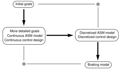
Figure 3: An overview of a complete development, starting with abstract goals, proceeding through explicit continuous and discrete deceleration models, and continuing with further low level models. Vertical arrows are (perhaps successive) model based refinements. Horizontal arrows are retrenchments, suited to relating models too different to be connected by refinement.

The complete process that we have in mind may be summarized in Fig. 3. The thick arrows trace a path through a family of models that a development route could plausibly take. The left hand side of the diagram concerns continuous models. At the start, we have high level requirements goals, expressed in a notation with formal underpinnings. We have in mind a formalism like KAOS [31, 32] (or more precisely, an adaptation of it to deal more honestly with continuous processes). These requirements goals can then be formally refined till they can be operationalized, i.e. transformed into the operations of a methodology such as ASM (again, adapted to deal with continuous evolution). Then comes our discretization step, necessitating the use of retrenchment. Once we have crossed the continuous/discrete boundary, we are free to revert to traditional model based refinement techniques for discrete state transition systems — no worries about continuous phenomena any more. In Fig. 3 we indicate how the discrete kinematics that we investigated earlier might be refined to a model of train braking, in which concern with the dynamics is replaced by a focus on the actuators that would implement the deceleration increments in practice.

Fig. 3 also features other models, indicated by asterisks. These are models whose existence is guaranteed by the Tower theorems [9, 29], making the squares of Fig. 3 commuting in an appropriate sense. However, we argue that these models are less useful than the others. Thus the lower left model would be a continuous version of the braking model, an unrealistic overidealisation so close to implementation. The upper right model would be a discretized version of the highest level requirements goals for train stopping. Again this would be inappropriate at such a high level, since it clutters what ought to be the most perspicuous expression of the system goals with a lot of material concerning low level details of the discretization scheme. This bears out what we said above about a combination of refinement and retrenchment techniques providing the best coverage of the route from high level requirements to low level implementation.

Above, we mentioned adaptations of KAOS and ASM to deal with continuous behaviour. We discuss these briefly now. Regarding ASM, a major part of what we need is already available in the literature, eg. [17, 40] which deal with (Real) Timed ASM. The essential observation is that in the context of continuous time, system states should be modeled as persisting over half-open half-closed time intervals, eg. $(t_{0},t_{1}]$. This allows the typical discontinuous state transition in a typical discrete transition system, say of a state variable $v$, to be represented as the move from $v(t_{0})$ (the value of $v$ at $t_{0}$, which lies outside $(t_{0},t_{1}]$ and is the right hand endpoint of the preceding interval), to $\lim_{\epsilon\rightarrow 0+}v(t_{0}+\epsilon)$ (the left hand limit at $t_{0}$ from the right, of values of $v$ within the interval $(t_{0},t_{1}]$). Likewise, a period of continuous evolution can be understood as persisting over such a half-closed interval, governed by a suitably well posed ODE initial value problem, and with the truth of the initial conditions for the initial value problem at the end of the preceding interval being the trigger for the system’s subsequently following a trajectory specified by the ODE problem. With these conventions, a version of ASM in which discrete steps alternate with continuous flows can be developed, reflecting many of the characteristics of hybrid automata.

A similar approach can be adopted for KAOS. Although KAOS depends on a notion of time from the outset, in the normal KAOS formalism, time is discrete, typically indexed by the integers, with requirements goals expressed as temporal logic formulae over time. For a version over continuous time, while some temporal operators, eg. always, until, offer no conceptual difficulties, the next operator needs to be rethought. Again half-open half-closed intervals, with successor states being defined via the limit from the right at the left hand end of a half-closed interval, can be used. To avoid problems arising due to an accumulation of next operators, syntactic restrictions have to be imposed on the permitted temporal formulae. However, the kinds of restrictions that need to be imposed are satisfied by the patterns that KAOS requirements are normally built out of.

8 Conclusion

In this paper we introduced a small continuous control problem in state space format, and then treated a discretized counterpart of it, utilising a zero order hold. Then came the main novel contribution of the paper, a rigorous treatment of the continuous to discrete modeling transformation, based on cited results from ODE theory. That done, we were able to integrate the results into a retrenchment which related from continuous and discrete models. As noted earlier, model based formal development normally starts already in the discrete domain, so the ability to connect this with the continuous world in a reasoned way, is a significant extension of the potential of model based formal techniques to underpin developments of such systems. Equally importantly, in making essential use of retrenchment to forge the connection between continuous modeling and discrete modeling, this work gives a fresh confirmation of the utility of the concept as a worthwhile adjunct to refinement in tackling the wider issues connected with real world formal developments.

Of course, this paper is by no means the last word in developments of this kind. As well as tackling a control problem that was almost trivial technically, the rigorous result from mathematical control theory that we utilized was relatively limited, insisting, as it did, that the two behaviours that were compared, started from the same state, using a rather crude $\mathcal{L}^{2}$ estimate of the difference in the control inputs to derive its conclusion, and being based on rather generic properties of the ODEs that govern the dynamics of the control problem. (These simple contraints also meant that relatively little of the expressive power of retrenchment was used in this case study.) In more realistic cases, the problem will be less amenable to analytic solution, and feedback mechanisms will help alleviate the inherent uncertainty that arises. Moreover, while a crude $\mathcal{L}^{2}$ estimate of the difference in the control inputs allows the two control inputs to get as far away from each other as the bounds on the control space allow, in practice, feedback mechanisms will tend to push them together, and this could be exploited to derive more stringent estimates of the difference between continuous and discrete control. All of this remains to be discussed in future work, as does the extension of the KAOS and ASM formalisms (or any alternatives that might be contemplated to act in their place), that can encompass the continuous behaviours that we have described.

Our work is to be contrasted with the possibilities offerd by the hybrid systems approach [43]. There, the insistence on (approximate) bisimulation between a continuous system and a discrete counterpart restricts attention to control systems which are stable in the Liapunov sense. In any event, the intense focus on considerations of algorithmic decidability in that field, with automata homomorphism as such a prominent relationship between system models, can inhibit design expressivity for the purposes that concern us. For instance, techniques that rely on stability, are, strictly speaking, not applicable to our simple case study.

Once a suitable collection of widely applicable and useful results of the kind discussed here have been established, the way is open for the incorporation of these into appropriate formal development tools. These would be of a different flavour to those typically developed for the hybrid systems field, since they would have more emphasis on interactive proving than is typically the case there. One snag that would have to be overcome is that most proving based tools cope rather badly with the kind of applied mathematics and rigorous analysis techniques that are required for this work. A notable exception is the PVS suite [18, 36], for which substantial library support exists to underpin both applied mathematics and its more rigorous counterparts, eg. [22]. This would be the obvious jumping off point for the development of tools that aligned well with our approach.

References

- [1]
- [2] J-R. Abrial (1996): The B-Book: Assigning Programs to Meanings. Cambridge University Press, 10.1017/CBO9780511624162.
- [3] J-R. Abrial (2010): Modeling in Event-B: System and Software Engineering. Cambridge University Press.
- [4] N. Ahmed (2006): Dynamic Systems and Control With Applications. World Scientific.
- [5] R. Alur, C. Courcoubetis, T. Henzinger & P-H. Ho (1993): Hybrid Automata: An Algorithmic Approach to the Specification and Verification of Hybrid Systems. In: Proc. Workshop on Theory of Hybrid Systems, LNCS 736, Springer, pp. 209–229.
- [6] R. Alur & D. Dill (1994): A Theory of Timed Automata. Theor. Comp. Sci. 126, pp. 183–235, 10.1016/0304-3975(94)90010-8.
- [7] P. Antsaklis & A. Michel (2006): Linear Systems. Birkhauser.
- [8] R. Banach: Model Based Refinement and the Design of Retrenchments. Available from [37].
- [9] R. Banach & C. Jeske: Retrenchment and Refinement Interworking: the Tower Theorems. Submitted.
- [10] R. Banach, C. Jeske & M. Poppleton (2008): Composition Mechanisms for Retrenchment. J. Log. Alg. Prog. 75, pp. 209–229, 10.1016/j.jlap.2007.11.001.
- [11] R. Banach, M. Poppleton, C. Jeske & S. Stepney (2007): Engineering and Theoretical Underpinnings of Retrenchment. Sci. Comp. Prog. 67, pp. 301–329, 10.1016/j.scico.2007.04.002.
- [12] S. Barnett (1975): Introduction to Mathematical Control Theory. Oxford University Press.
- [13] E. Börger (2003): The ASM Refinement Method. F.A.C.J. 15, pp. 237–257.
- [14] E. Börger & R.F. Stärk (2003): Abstract State Machines. A Method for High Level System Design and Analysis. Springer.
- [15] F. Clarke (1987): Optimization and Nonsmooth Analysis. Society for Industrial Mathematics.
- [16] F. Clarke, Y. Ledyaev, R. Stern & P. Wolenski (1997): Nonsmooth Analysis and Control Theory. Springer.
- [17] J. Cohen & A. Slissenko (2008): Implementation of Timed Abstract State Machines with Instantaneous Actions by Machines with Delays. Technical Report TR-LACL-2008-2, LACL, University of Paris-12.
- [18] J. Crow, S. Owre, J. Rushby, N. Shankar & M. Srivas (1995): A Tutorial Introduction to PVS. In R. France, S. Gerhart & M. Larrondo-Petrie, editors: WIFT’95: Workshop on Industrial-Strength Formal Specification Techniques, IEEE Computer Society Press.
- [19] J. D’Azzo & C. Houpis (1995): Linear Control System Analysis and Design: Conventional and Modern. McGraw Hill.
- [20] J Derrick & E Boiten (2001): Refinement in Z and Object-Z: Foundations and Advanced Applications. Springer-Verlag UK, 10.1007/978-1-4471-0257-1.
- [21] R. Dorf & R. Bishop (2010): Modern Control Systems. Pearson.
- [22] B. Dutertre (1996): Elements of Mathematical Analysis in PVS. In: TPHOLS 1996, LNCS 1125, Springer.
- [23] K. Dutton, S. Thompson & B. Barraclough (1997): The Art of Control Engineering. Addison Wesley.
- [24] M. Fadali & A. Visioli (2009): Digital Control Engineering: Analysis and Design. Academic Press.
- [25] G. Franklin, J. Powell & M. Workman (1996): Digital Control Systems. Prentice Hall.
- [26] J. He (1994): From CSP to hybrid systems. In A.W. Roscoe, editor: A Classical Mind, Essays in Honour of C.A.R. Hoare, Prentice-Hall International, pp. 171–189.
- [27] T. A. Henzinger (1996): The Theory of Hybrid Automata. In: Proc. IEEE LICS-96, IEEE, pp. 278–292. See also http://mtc.epfl.ch/~tah/Publications/the_theory_of_hybrid_automata.pdf.
- [28] IEEE Standard 1474: IEEE Standard for Communications-Based Train Control (CBTC) Performance and Functional Requirements: IEEE Std 1474.1-2004; IEEE Standard for User Interface Requirements in Communications-Based Train Control (CBTC) Systems: IEEE Std 1474.2-2003; IEEE Recommended Practice for Communications-Based Train Control (CBTC) System Design and Functional Allocations: IEEE Std 1474.3-2008.
- [29] C. Jeske (2005): Algebraic Integration of Retrenchment and Refinement. Ph.D. thesis, University of Manchester.
- [30] B. Kuo (1992): Digital Control Systems. Oxford University Press.
- [31] A. van Lamsweerde (2009): Requirements Engineering: From System Goals to UML Models to Software Specifications. Wiley.
- [32] Letier, E. (2001): Reasoning about Agents in Goal-Oriented Requirements Engineering. Ph.D. thesis, Dépt. Ingénierie Informatique, Université Catholique de Louvain.
- [33] K. Ogata (2008): Modern Control Engineering. Pearson.
- [34] P. Paraskevopoulos (1996): Digital Control Systems. Prentice Hall.
- [35] B Potter, J Sinclair & D Till (1996): An Introduction to Formal Specification and Z, 2nd. edition. Prentice Hall.
- [36] PVS Homepage: http://pvs.csl.sri.com.
- [37] Retrenchment Homepage: http://www.cs.man.ac.uk/retrenchment.
- [38] W P de Roever & K Engelhardt (1998): Data Refinement: Model-Oriented Proof Methods and their Comparison. Cambridge University Press.
- [39] E Sekerinski & K Sere (1998): Program Development by Refinement: Case Studies Using the B-Method. Springer.
- [40] A. Slissenko & P. Vasilyev (2008): Simulation of Timed Abstract State Machines with Predicate Logic model Checking. J.U.C.S. 14, pp. 1984–2006.
- [41] E. Sontag (1998): Mathematical Control Theory. Springer.
- [42] W. Su, F. Yang, X. Wu, J. Gou & H. Zhu (2011): Formal Approaches to Mode Conversion and Positioning for Vehicle Systems. In: Proc. 3rd IEEE International Workshop on Security Aspects of Process and Services Engineering. To appear.
- [43] P. Tabuada (2009): Verification and Control of Hybrid Systems: A Symbolic Approach. Springer.
- [44] J Woodcock & J Davies (1996): Using Z, Specification, Refinement and Proof. Prentice Hall.