Model exploration and analysis for quantitative safety refinement in probabilistic B

Abstract

The role played by counterexamples in standard system analysis is well known; but less common is a notion of counterexample in probabilistic systems refinement. In this paper we extend previous work using counterexamples to inductive invariant properties of probabilistic systems, demonstrating how they can be used to extend the technique of bounded model checking-style analysis for the refinement of quantitative safety specifications in the probabilistic B language. In particular, we show how the method can be adapted to cope with refinements incorporating probabilistic loops. Finally, we demonstrate the technique on pB models summarising a one-step refinement of a randomised algorithm for finding the minimum cut of undirected graphs, and that for the dependability analysis of a controller design.

Keywords Probabilistic B, quantitative safety specification, refinement, counterexamples.

1 Introduction

The B method [2] and more recently its successor Event-B [3] comprises a method and its automation for modelling complex software systems. It is based on the top-down refinement where specifications can be elaborated with detail and additional features, whilst the automated prover checks consistency between the refinements. Hoang’s probabilistic B or pB [16] extension of standard B gave designers the ability to refer to probability and access to the specification of quantitative safety properties.

In probabilistic systems, the generalisation of traditional safety properties allows the specification of random variables whose expected value must always remain above some given threshold. Elsewhere [24, 26] we have provided automation to check this requirement by analysing pB models using an automatic translation of their quantitative safety specifications as PRISM reward structures [15]. Our technique allows pB modellers to explore the quantitative safety properties encoded within their models to obtain diagnostic feedback in the form of counterexample traces in the case that their model does not satisfy the quantitative specification. Counterexamples become sets of execution traces each with some probability of occurring and jointly implying that the specified threshold is not maintained. Moreover pB’s consistency checking enforces inductive invariance of the quantitative safety property, thus the counterexample traces also demonstrate specific points in the models execution where the inductive property fails.

The paradigm of abstraction and refinement supports stepwise development of probabilistic systems aimed at improving probabilistic results. Unfortunately, for quantitative safety specifications (our focus here), a human verifier has no way of inspecting that this requirement is met even though the automated prover readily establishes consistency between the refinements. One way to resolve this uncertainty is to explore algorithmic approaches similar to probabilistic model checking techniques which can provide exact diagnostics summarising the failure (if indeed it exists) of the refinement goal.

In this paper we extend some practical uses of counterexamples to probabilistic systems refinement with respect to quantitative safety specifications particular to the pB language. We show how to use them to generalise bounded model checking-style analysis for probabilistic programs so that an iteration can be verified by exhaustive search provided that quantitative invariants are inductive for all reachable states. We also show how the use of probabilistic counterexamples in quantitative dependability analysis can be used to determine “failure modes” and “critical sets” which thus enables their extension to estimating components severity.

We illustrate the techniques on two case studies: one based on a probabilistic algorithm [21] to find the minimum cut set in a graph, and the other a probabilistic design for a controller mechanism [12].

The outline of the paper is as follows. In Sec.2 we summarise the underlying theory of pB; in Sec.3 we discuss the probabilistic counterexamples we can derive from the models and a bounded model checking approach to probabilistic iteration. In Sec.5 we illustrate the technique on the specification of a randomised “min-cut”. We discuss probabilistic diagnostics of dependability in Sec.6 and demonstrate with a case study in Sec.7. We discuss related work and then conclude.

1.0.1 Notation

Function application is represented by a dot, as in $f.x$ (rather than $f(x)$). We use an abstract finite state space $S$. Given predicate pred we write liftpred for the characteristic function mapping states satisfying pred to $1$ and to $0$ otherwise, punning $1$ and $0$ with “True” and “False” respectively. We write ${\cal E}S$ as the set of real-valued functions from $S$, i.e. the set of expectations; and whenever $e,e^{\prime}\in{\cal E}S$ we write $e\Rrightarrow e^{\prime}$ to mean that $\mathord{(\forall s\in S.\ e.s\leq e^{\prime}.s)}$. We let $\mathbb{D}S$ be the set of all discrete probability distributions over $S$; and write $\mathord{Exp.\delta.e=\displaystyle\sum_{s\in S}(\delta.s)\times e.s}$ for the expected value of $e$ over $S$ where $\delta\in\mathbb{D}S$ and $e\in{\cal E}S$. Finally we write $S^{\ast}$ for the finite sequences of states in $S$.

2 Probabilistic annotations

When probabilistic programs execute they make random updates; in the semantics that behaviour is modelled by discrete probability distributions over possible final values of the program variables. Given a program Prog operating over $S$ we write $[\![\textit{Prog}]\!]:S\rightarrow(S\rightarrow[0,1])$ for the semantic function taking initial states to distributions over final states. For example, the program fragment

$$\textit{pInc}\ \triangleq\ s{:}{=}\,s{+}1\ \mathbin{\makebox[0.0pt]{~{}}_{p}\oplus}\ s{:}{=}\,s{-}1$$ (1)

increments state variable $s$ with probability $p$, or decrements it with probability $1{-}p$. The semantics $[\![\textit{pInc}]\!]$ for each initial state $s$ is a probability distribution returning $p$ or $(1{-}p)$ for (final) states $s^{\prime}=(s{+}1)$ or $s^{\prime}=(s{-}1)$ respectively. Rather than working with this semantics directly, we shall focus on the dual logical view generalisation of Hoare logic [17].

Probabilistic Hoare logic [23] takes account of the probabilistic judgements that can be made about probabilistic programs, in particular it can express when predicates can be established only with some probability. However, as we shall see, it is even more general than that, capable of expressing general expected properties of random variables over the program state. We use Real-valued annotations of the program variables interpreted as expectations; a program annotation is said to be valid exactly when the expected value over the post-annotation is at least the value given by the pre-annotation. In detail

$$\{\textit{pre}\}~{}~{}\textit{Prog}~{}~{}\{\textit{post}\}~{},$$ (2)

is valid exactly when $\textit{Exp}.[\![\textit{Prog}]\!].\textit{post}.s\geq\textit{pre}.s$ for all states $s\in S$, where post is interpreted as a random variable over final states and pre as a real-valued function.

With our notational convention, a correct annotation for pInc (at (1)) is given by the triple

$$\{p\times\textsf{lift}{(s=-1)}+(1{-}p)\times\textsf{lift}{(s=1)}\}~{}~{}~{}~{}\textit{pInc}~{}~{}~{}~{}\{\textsf{lift}{(s=0)}\}~{},$$ (3)

which expresses the probability of establishing the state $s=0$ finally, depending on the initial state from which pInc executes. Thus if the initial state is $s=-1$ then that probability is $p$, but it is $(1{-}p)$ if the initial state is $s=1$.

Rather than use the distribution-centered semantics outlined above, we shall use a generalisation of Dijkstra’s weakest precondition or Wp semantics defined on the program syntax of the probabilistic Guarded Command Language or pGCL [23]. The semantics of the language is set out in Fig. 1. As for standard Wp this formulation allows annotations to be checked mechanically [16, 18]; moreover we see that annotation (2) is valid exactly when $\textit{pre}\Rrightarrow\textit{Wp}.{\textit{Prog}}.{\textit{post}}$.

$$\small\begin{array}[]{lll}Name&\textit{Prog}&\textit{Wp}.{\textit{Prog}}.{\textit{Expt}}\\ \hline\cr\\ \mbox{identity}&\mbox{{skip}}&\mbox{$\textit{Expt}$}\\ \mbox{assignment}&\mbox{$x:=f$}&\mbox{$\textit{Expt}[x:=f]$}\\ \mbox{composition}&\mbox{{$Prog;Prog^{\prime}$}}&\mbox{$\textit{Wp}.{Prog}.{(wp\cdot{Prog^{\prime}}\cdot{\textit{Expt}})}$}\\ \mbox{choice}&\mbox{$Prog\,\,\mbox{$\lhd$}\ G\ \mbox{$\rhd$}\ Prog^{\prime}$}&\mbox{$\textit{Wp}.{Prog}.{\textit{Expt}}\,\,\mbox{$\lhd$}\ G\ \mbox{$\rhd$}\ \textit{Wp}.{Prog^{\prime}}.{\textit{Expt}}$}\\ \mbox{probability}&\mbox{$Prog\mathbin{\makebox[0.0pt]{~{}}_{p}\oplus}\ Prog^{\prime}$}&\mbox{$\textit{Wp}.{Prog}.{\textit{Expt}}\ \mathbin{\makebox[0.0pt]{~{}}_{p}\oplus}\ \textit{Wp}.{Prog^{\prime}}.{\textit{Expt}}$}\\ \mbox{nondeterminism}&\mbox{${Prog\ ~{}\sqcap~{}\ Prog^{\prime}}$}&\mbox{$\textit{Wp}.{Prog}.{\textit{Expt}}\ $min$\ \textit{Wp}.{Prog^{\prime}}.{\textit{Expt}}$}\\ \mbox{weak iteration}&\mbox{{\sf it}\ $Prog$ \ {\sf ti}}&\mbox{$\nu X\bullet(\textit{Wp}.{Prog}.{X}\ $min$\ \textit{Expt})$}\\ \\ \hline\cr\\ \end{array}$$

Given a program command $Prog$ and expectation Expt of type ${\cal E}S$, $\textit{Wp}.\textit{Prog}$ is of type ${\cal E}S\rightarrow{\cal E}S$. Note also that we write $\textit{Exp}.([\![\textit{Prog}]\!].s).\textit{Expt}$ to mean $\textit{Wp}.\textit{Prog}.\textit{Expt}.s.$

Figure 1: Structural definition of the expectation transformer-style semantics.

In this paper we shall concentrate on certifying probabilistic safety expressible using probabilistic annotations. Informally, a probabilistic safety property is a random variable whose expected value cannot be decreased on execution of the program. (This idea generalises standard safety, where the truth of a safety predicate cannot be violated on execution of the program.) Safety properties are characterised by inductive invariants: for example the valid annotation $\{\textit{Expt}{\times}\textsf{lift}{\textit{pred}}\}~{}\textit{Prog}~{}\{\textit{Expt}\}$ says that Expt is an inductive invariant for Prog provided it is executed in an initial state satisfying pred. To illustrate, the annotation

$$\{s\}~{}~{}~{}~{}\textit{pInc}~{}~{}~{}~{}\{s\}~{},$$ (4)

means that the expected value of $s$ is never decreased (and it is therefore only valid if $p\geq 1/2$).

Inductive invariants will be a significant component of the refinement of quantitative safety specifications in our pB machines, to which we now turn.

2.1 Probabilistic safety and refinement in pB

Probabilistic B or pB [16], is an extension of standard B [2] to support the specification and refinement of probabilistic systems. Systems are specified by a collection of pB machines which consist of operations describing possible program executions, together with variable declarations and invariants prescribing correct behaviour.

The machine set out in Fig. 2 illustrates some key features of the language. There are two operations –OpX and OpY– which can update a variable $cc$. OpX can either increment cc by 1 or decrement it by the same value with probability $p$ or $(1-p)$ respectively, while OpY just resets the current value of cc to 0. In general, operations can execute only if their preconditions hold. But in the absence of preconditions as in this case, the choice of which operation to execute is made nondeterministically.

The remaining clauses ascribe more information to the variables, constants and behaviour of the operations. Declarations are made in the CONSTANTS and VARIABLES clauses; PROPERTIES and SEES clauses state assumed properties and context of the constants and variables. The INVARIANT clause sets out invariant properties. The expression in the INITIALISATION clause must establish the invariant and the operations OpX and OpY must maintain it afterwards.

We shall concentrate on the EXPECTATIONS clause, which was introduced by Hoang [16] to express quantitative invariant or safety properties. The form of an EXPECTATIONS clause is given by

MACHINE	Faulty
SEES	Int_TYPE, Real_TYPE
CONSTANTS	$p$
PROPERTIES	$p\in REAL\wedge p\geq real(0)\wedge p\leq real(1)$
VARIABLES	$cc$
INVARIANT	$cc\in\mathbb{N}$
INITIALISATION	$cc:=0$
OPERATIONS
	OpX $\ \triangleq\$ BEGIN
	PCHOICE  $p$  OF  $cc:=cc+1$
	OR  $cc:=cc-1$  END;
	OpY $\ \triangleq\$ $cc:=0$
EXPECTATIONS	$real(0)\ \Rrightarrow\ cc$
END

Bold texts on the left column capture the fields (or clauses) used to describe the machine. The PCHOICE keyword introduces a probabilistic binary operator; the EXPECTATIONS clause expresses the notion of probabilistic quantitative safety.

Figure 2: A simple pB machine.

$$E\Rrightarrow\textit{Expt}~{},$$ (5)

where both $E$ and Expt are expectations. It specifies that the expected value of Expt should always be at least $E$, where the expected value is determined by the distribution over the state space after any valid execution of the machine’s operations, following its initialisation. Hoang showed that this is guaranteed by the following valid annotations:

$$\{E\}~{}~{}~{}\textit{init}~{}~{}~{}\{\textit{Expt}\}~{}~{}~{}\quad\textit{and}~{}~{}~{}\quad\{\textsf{lift}{\textit{pred}}{\times}\textit{Expt}\}~{}~{}~{}\textit{Op}~{}~{}~{}\{\textit{Expt}\}~{},$$ (6)

where Op is any operation with precondition pred and init is the machine’s initialisation. In what follows we shall refer to (6) as the proof obligations for the associated expectations clause (5).

Checking the validity of program annotation, and in particular inductive invariants for loop-free program fragments can be done mechanically based on the semantics set out in Fig. 1. In some cases the proof obligation cannot be discharged, and there are two possible reasons for this. The first possibility is that Expt is too weak to be an inductive invariant for the machine’s operations, and must be strengthened by finding $\textit{Expt}^{\prime}\Rrightarrow\textit{Expt}$ so that the original safety property can be validated. The second possibility is that the machine’s operations actually violate the probabilistic safety property.

The same reasoning can be extended to refinement of abstract pB machines. We note that quantitative safety specifications in pB can also be refined in the usual way with respect to expectation pairs. Thus another way of expressing (5) is to say that any program command $P$ satisfies the bounded expectation pair $[E,\textit{Expt}]$ if execution from its initial state guarantees that

$$E\Rrightarrow\textit{Wp}.{P}.\textit{Expt}.$$ (7)

Refinement is then implied by the ordering of program commands so that more refined programs improve probabilistic results. More specifically, we write

$$\mathord{P\ref{Q}~{}~{}~{}\textit{iff}~{}~{}~{}(\forall E\in{\cal E}{S}\mbox{\boldmath$\cdot$}\textit{Wp}.P.E\Rrightarrow\textit{Wp}.Q.E)},$$ (8)

to mean that the program command $Q$ is a refinement of the program command $P$. In addition we note that the preservation of an expression like (5) is implied by the monotone property of Wp.

The refinement of abstract pB machines embedding quantitative safety statements is dealt with in the language framework by introducing the IMPLEMENTATION and REFINES clauses. The former clause specifies the refinement of an abstract machine specified in the latter clause. The refinement process is then aimed at preserving the bounds of expectations in the original specification statement (the machine to be refined) so that the validity of an expression like (6) can be checked mechanically.

Our aim in the next section is to use probabilistic counterexamples adopted in model checking techniques to interpret failure of proofs of refinement of probabilistic machines in the pB language. We will find that a counterexample is a trace (or a set of traces) from the initialisation to a state where the inductive invariant fails to hold after inspecting the EXPECTATIONS clause over the refinement.

3 Probabilistic safety in Markov Decision Processes

In abstract terms pGCL  programs and pB machines may be modelled as a Markov Decision Process (MDP). Recall that an MDP combines the notion of probabilistic updates together with some arbitrary choice between those updates [28]: that combination of probabilistic choices together with nondeterministic choices is present in pGCL  and captures both features.

In this section we summarise pB models and their quantitative safety specifications in terms of MDPs, and show how to apply model checking’s search techniques for counterexamples to prove quantitative safety as a first step towards generalising standard bounded model checking verification. Inductive invariance is then crucial to the application of exhaustive state exploration for the intended goal.

Here we consider an MDP expressed as a nondeterministic selection $\mathord{P\ \triangleq\ P_{0}~{}\sqcap~{}\dots~{}\sqcap~{}P_{n}}$ of deterministic pGCL  programs, where the nondeterminism corresponds to the arbitrary choice, and each $P_{i}$ corresponds to the probabilistic update for a choice $i$. When $P$ is iterated for some arbitrarily-many steps, we identify a computation path as a finite sequence of states $\langle s_{0},s_{1},s_{2},\dots,s_{n}\rangle$ where each $(s_{i},s_{i+1})$ is a probabilistic transition of $P$, i.e. $s_{i+1}$ can occur with non-zero probability by executing $P$ from $s_{i}$. Note that the choice (between $0\dots n$) can depend on the previous computation path since for example guards for the individual operations $P_{i}$ must hold for their selection to be enabled.

Standard safety properties identify a set of “safe” states — the safety property then holds provided that all states reachable from the initial state under specified state transitions are amongst the selected safe states. A generalisation of this for probabilistic systems specifies thresholds on the probability for which the reachable states are always amongst the safe states. The quantitative safety properties encapsulated by the EXPECTATIONS clause are even more general than that, allowing the possibility to specify thresholds on arbitrary expected properties. The next definition sets out the mathematical model for interpreting general quantitative safety properties.

Since MDPs contain both nondeterministic and probabilistic choice, taking expected values only makes sense over well-defined probability distributions — we need to resolve the nondeterministic choice in all possible ways to yield a set of probability distributions. The next definition sets out a mechanism for doing just that.

Definition 1

Given a program $P$, an execution schedule is a map $\aleph:S^{*}\rightarrow{\mathbb{D}}$S so that $\aleph.\alpha\in[\![P]\!].s$ picks a particular resolution of the nondeterminism in $P$ to execute after the trace $\alpha$, where $s$ is the last item of $\alpha$. (A more uniform formalisation would give the distribution of initial states as $\aleph.\langle\rangle$; but we prefer to give initial states explicitly.)

Once a particular schedule has been selected, the resulting behaviour generates a probability distribution over computation path. We call such a distribution a probabilistic computation tree; such distributions are well-defined with respect to Borel algebras based on the traces.

Definition 2

Given a program $P$, initial state $s_{0}$ and execution schedule $\aleph$, we define the corresponding trace distribution $\langle\!|P_{\aleph}|\!\rangle.s_{0}$ of type $S^{*}\rightarrow[0,1]$ to be

$$\begin{array}[]{lrcl}&\langle\!|P_{\aleph}|\!\rangle.s_{0}.(s^{\prime})&\ \triangleq&1~{}\textrm{if}~{}s^{\prime}=s_{0}~{}\textrm{else}~{}0\\ \textrm{and}&\langle\!|P_{\aleph}|\!\rangle.s_{0}.(\alpha ss^{\prime})&\ \triangleq&\langle\!|P_{\aleph}|\!\rangle.s_{0}.(\alpha s){\times}{\aleph.(\alpha s)}.s^{\prime}\end{array}$$

Computation trees of finite depth generate a distribution over endpoints as follows. If we take $K$ steps from some initial $s_{0}$ according to the schedule $\aleph$, then the probability of ending in state $s^{\prime}$ is given by

$$[\![P^{K}_{\aleph}]\!].s_{0}.s^{\prime}\ \triangleq\ \sum_{|\alpha|=K}\langle\!|P_{\aleph}|\!\rangle.s_{0}.(\alpha s^{\prime})~{}.$$

General quantitative safety properties are intuitively specified via a numeric threshold $e$ and a random variable Expt over the state space $S$: the expected value of Expt with respect to any distribution over endpoints should never fall below the threshold $e$.

Definition 3

Given threshold $e$ and an expectation Expt the general quantitative safety property is satisfied by the program $P$ if for all schedules $\aleph$ and $K\geq 0$, we have that $\textit{Exp}.[\![P^{K}_{\aleph}]\!].\textit{Expt}.s_{0}\geq e$.

The probabilistic Computation Tree Logic or pCTL [14] safety property, which places a threshold on the probability that the reachable states always satisfy the identified “safe” states is expressible using Def. 3 via characteristic expectation $\textsf{lift}{safe}$. However many more general properties are also expressible, including expected time complexity [15].

We shall be interested in identifying situations where the inequality in Def. 3 does not hold. Evidence for the failure is a (finite) computation tree whose distribution over endpoints illustrates the failure to meet the threshold.

Definition 4

Given a probabilistic safety property, a failure tree is defined by a scheduler $\aleph$ and an integer $K\geq 0$ such that $\textit{Exp}.[\![P^{K}_{\aleph}]\!].\textit{Expt}.s_{0}<e$.

Elsewhere [25] we showed that if Expt is an inductive invariant, then the safety property based on Expt is implied, provided that $e\leq\textit{Expt}.s_{0}$. In fact, given a failure tree, there must be some finite trace $\alpha$ such that $\langle\!|P_{\aleph}|\!\rangle.s_{0}.(\alpha s)>0$ and $\textit{Wp}.(P~{}\sqcap~{}\textbf{skip}).\textit{Expt}.s<\textit{Expt}.s$ [25]. Thus, as for standard model checking, we are able to locate specific traces which lead to the failure of the invariant property. We define a counterexample to inductive invariance as follows.

Definition 5

Given a scheduler $\aleph$, an expectation Expt and a program $P$, a counterexample to inductive invariance safety property is a trace $(\alpha s)$ which can occur with non-zero probability, and such that $\textit{Wp}.P.\textit{Expt}.s<\textit{Expt}.s$. A state such as s is a witness to failure.

But note that in practice there will be a number of counterexamples. Our technique is able to identify them all given any depth $K$ of computation. Next we discuss how the strategy can be extended to probabilistic loops reasoning.

3.1 Analysis of loops

We assume a loop of the form $\textit{loop}\ \triangleq\ \textbf{while}\ G\ \textbf{do}\ body\ \textbf{od}\,$ where $G$ is a predicate over the program state representing the loop guard; $body$ is a probabilistic program consisting of a finite nondeterministic choice over probabilistic updates. Our aim in this section is to generalise the technique of bounded model checking to prove the safety assertion of the form

$$\{e\}~{}~{}\textit{loop}~{}~{}\{\textit{inv}\}~{}.$$ (9)

In the case that (9) does not hold there must be a failure tree (Def. 4) to witness that fact, together with a set of failures to inductive invariance of inv. We shall be interested in the complementary problem, in the case that the property does hold. For standard programs this can be established by exhaustively searching the reachable states; any revisiting of a state terminates the search at that point, so that the method is complete for finite state programs: either a counterexample is discovered or all reachable states are visited, and each one checked for satisfaction of the (qualitative) safety property.

The situation is not quite so straightforward for probabilistic programs, and that is because the technique of exhaustive search does not generalise immediately to quantitative safety properties. However via inductive invariants it does. Consider the program which repeatedly sets a variable $x$ uniformly in the set $\{0,1,2\}$ after the initialisation $x:=1$, and terminates whenever $x$ is set to $2$. In this case we might like to verify the safety property that $x\in\{1,2\}$ with probability at least $1/2$. Expressed as an assertion, it becomes

$$\{1/2\}~{}~{}~{}~{}~{}~{}~{}\begin{array}[]{l}x:=1;\textbf{while}~{}(x=1)~{}\textbf{do}~{}~{}~{}x{:}{=}\,0\mathbin{\makebox[0.0pt]{~{}}_{1/3}\oplus}(x{:}{=}\,1\mathbin{\makebox[0.0pt]{~{}}_{1/2}\oplus}x{:}{=}\,2)~{}\textbf{od}\end{array}~{}~{}~{}~{}~{}~{}\{\textit{post}\}~{},$$ (10)

where $\textit{post}\ \triangleq\ \{\textsf{lift}{(x\in\{1,2\})}\}$. A quantitative inductive invariant establishing that fact is given by $x/2$, expressing the probability that the safety property is always satisfied at that state. (When $x$ is $2$ that probability is $1$, when $x$ is $1$, it is $1/2$ and when $x$ is $0$ it is $0$.) In fact the property (10) is equivalently formulated by setting $\textit{post}\ \triangleq\ x/2$, which can be seen as a strengthening of $\{\textsf{lift}{(x\in\{1,2\})}\}$.

Since the triple (10) does indeed hold, no failure trees exist; more generally, in standard model checking and for finite state spaces such a failure to establish the presence of a failure tree can be converted to a proof that the property holds (provided all reachable states are examined). For probabilistic systems however, it is not clear when to terminate a state exploration, since $\textit{Exp}.[\![\textit{body}^{K}_{\aleph}]\!].x/2$ steadily approaches $1/2$ from above (where here body is taken to be the guarded loop body of (10)). However we can recover the termination property even for probabilistic systems by looking at inductive invariants, as the next lemma shows.

Lemma 1

Let $P$ be a probabilistic program operating over a finite state space $S$; let $s_{0}$ be the initial state. If for all states $s$, reachable from $s_{0}$ under executions via $P$, the inductive invariance property $\textit{Wp}.P.\textit{inv}.s\geq\textit{inv}.s$ holds, then $\textit{Exp}.[\![P^{K}_{\aleph}]\!].\textit{inv}\geq\textit{inv}.s_{0}$ for all $K$ and schedules $\aleph$.

Proof 1

(Sketch) We use proof by induction on $K$.

When $K=1$ we note that $\textit{Exp}.[\![P^{1}_{\aleph}]\!].\textit{inv}\geq\textit{inv}.s_{0}$ is a consequence of the assumption since $\textit{Exp}.[\![P^{1}_{\aleph}]\!].\textit{inv}\geq\textit{Wp}.P.\textit{inv}.s_{0}$.

For the general step, we observe similarly that $\textit{Exp}.[\![P^{K+1}_{\aleph}]\!].\textit{inv}\geq\textit{Exp}.[\![P^{K}_{\aleph}]\!].(\textit{Wp}.P.\textit{inv})$. The result follows through monotonicity of the expectation operator.

Lem. 1 implies that we can use exhaustive search to verify quantitative safety properties using inductive invariants and exhaustive state exploration. The search terminates once all reachable states have been verified as satisfying the inductive property. In the case of (10), using $x/2$ for the invariant, each of the three states satisfies the inductive property. Next we summarise a prototype tool framework for locating and presenting counterexamples.

4 Automating counterexamples generation

YAGA [26] is a prototype suite of programs for inspecting safety specifications of abstract pB machines and their refinements. Importantly, it allows a pB machine designer to explore experimentally the details of system construction in order to ascertain the cause(s) of failure of a pB safety encoding as in (5).

YAGA inputs a pB machine or its refinement violating a specific safety property expressed in its EXPECTATIONS clause, and generates its equivalent MDP representation in the PRISM language [15]. PRISM is a probabilistic model checker that permits pB models as MDPs in the tool framework and thus can investigate critical expected values of random variables as “reward structures” — a part of PRISM’s specification language. PRISM can then be used to explore the computation of $\textit{Exp}.[\![P_{\aleph}^{K}]\!].\textit{Expt}.s_{0}$ for values of $K\geq 0$, and thus (modulo computing resources) can determine values of $K$ for which the expectations clause fails. If such a $K$ is discovered, YAGA is able to extract the resultant failure tree as an “extremal scheduler” that fails the inductivity test. The extremal scheduler is a transition probability matrix which gives a description of the best (or worst-case) deterministic scheduler of the PRISM representation of an abstract ‘faulty’ pB machine — i.e. one whose probability (or reward) of reaching a state where our intended safety specification is violated is maximal (or minimal).

Finally, YAGA analyses the resultant extremal scheduler using algorithmic techniques set out in [25] and generates ‘the most useful’ diagnostic information composed of finite execution traces as sequences of operations and their state valuations leading from the initial state of the pB machine to a state where the property is violated. Details of the underlying theory of YAGA, its algorithms and implementation can be found elsewhere [26, 25]. In the next section we discuss practical details on how to use exhaustive search of pB machines to verify compliance of inductivity for finite probabilistic models.

5 Case study one: min-cut

We discuss one of Hoang’s pB models [16]: a randomised solution to finding the “minimum cut” in an undirected graph. The probabilistic algorithm is originally due to Karger [21]. We also report experimental results after running our diagnostic tool.

Let an undirected graph be given by $(N,E)$ where $N$ is a set of nodes and $E$ is a set of edges. The graph is said to be disconnected if $N$ is a disjoint union of two nonempty sets $N_{0},N_{1}$ such that any edge in $E$ connects nodes in $N_{0}$ or $N_{1}$; a graph is connected if it is not disconnected. A cut in a connected graph is a subset $E^{\prime}\subseteq E$ such that $(N,E\backslash E^{\prime})$ is disconnected; a cut is minimal if there is no cut with strictly smaller size. Cuts are useful in optimisation problems but are difficult to find. Karger’s algorithm uses a randomisation technique which is not guaranteed to find the minimal cut, but only with some probability.

$\begin{array}[]{ll}\hline\cr\\ \noindent\mbox{{\bf IMPLEMENTATION}}&\mbox{contractionImp}\\ \mbox{{\bf REFINES}}&\mbox{contraction}\\ \mbox{{\bf SEES}}&\mbox{Bool\_Type, Int\_TYPE, Real\_TYPE}\\ \mbox{\bf OPERATIONS}&\\ \quad\quad\mbox{ans $\longleftarrow$ {\bf contraction} ($NN$) $\ \triangleq\ $ }&{\bf VAR}\ $nn$\ {\bf IN}\\ \quad\quad\quad\quad\mbox{{\bf}}&\mbox{$nn:=NN;ans:=TRUE;$}\\ \\ &\mbox{{\bf WHILE} (nn $>$ 2) {\bf DO}}\\ &\mbox{$ans\longleftarrow{\bf merge}(nn,ans)$;}\\ &\mbox{$nn:=nn-1$ }\\ &\mbox{{\bf VARIANT} {\quad$nn$}}\\ &\mbox{{\bf INVARIANT} {$nn\in\mathbb{N}\wedge nn\leq NN\wedge 2\leq nn\wedge ans\in BOOL\ \wedge$}}\\ &\mbox{$expectation(frac(2,nn\times(nn-1))\times\textsf{lift}{ans})$}\\ \mbox{{\bf END;}}\\ \mbox{{\bf END}}&\\ \hline\cr\end{array}$ .

Figure 3: A pB refinement of the contraction specification of the Mincut algorithm.

The idea of the algorithm is to use a “contraction” step, where first an edge $e$ connecting two nodes $(n_{1},n_{2})$ is selected at random and then a new graph created from the old by “merging” $n_{1}$ and $n_{2}$ into a single node $n_{12}$; edges in the merged graph are the same as in the original graph except for edges that connected either $n_{1}$ or $n_{2}$. In that case if $(n_{1},a)$, say was an edge in the original graph then $(n_{12},a)$ is an edge in the merged graph. We keep merging while the number of nodes is greater than 2. The specification of the merge function for an initial number of nodes $NN$ is such that

$$ans\longleftarrow{\bf merge}(nn,aa)\ \triangleq\ nn\in NN\wedge aa\in BOOL\ |\ ans:=({\bf false}\ _{\leq\mathbin{\makebox[0.0pt]{~{}}_{2/nn}\oplus}}\ aa).$$

It expresses that with a probability of at most $2/nn$, the minimum cut will be destroyed by the contraction step. Otherwise the minimum cut is guaranteed to be found. Contraction satisfies an interesting combinatorial property which is that if the edge is chosen uniformly at random from the set of edges then the merged graph has the same minimum cut as does the unmerged graph with probability at least $2/(NN(NN{-}1))$. Although this probability can be small, it can be amplified by repeating the algorithm to give a probability of assurance to within any specified threshold.

The pB implementation in Fig. 3 sets out part of the refinement step for the min-cut algorithm. The refinement describes an iteration where the merge function is called to perform the contraction described above. The result of a call to merge is that the number of nodes in the graph (given by the variable $nn$) is diminished by $1$ and either the original minimum cut is preserved (with probability mentioned above), or it is not; the Boolean ans is used to indicate which of these possibilities has been selected.

Here we use the $expectation(.)$ function to check that the expression $\textsf{lift}{ans}\times 2/(nn(nn{-}1))$ simplifies to an inductive property; that is, that the probability of preserving the minimum cut should always be at least $2/(nn(nn{-}1))$ while $ans$ remains true, but is $0$ if $ans$ ever becomes false. Note that if this property holds then we are able to deduce exactly that the overall probability that the original minimum cut is preserved when the graph is merged to one of $2$ nodes is the theoretically predicted $2/(NN(NN{-}1))$.

Next we describe bounded model checking style experiments to analyse the refinement.

5.1 Experiments for min cut

5.1.1 Counterexample diagnostics

In our first experiment we introduce an error in the design of the merge function. The graph depicted in Fig. 4 shows a failure to preserve the expected probability threshold of the mincut algorithm. Specifically the graph shows that the probability falls below $2/(NN(NN{-}1))$. An examination of the resultant failure tree produces the counterexample depicted in Fig. 5. It clearly reveals a problem ultimately leading to a witness after executing the merge operation.

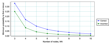
Figure 4: Graph comparing the probabilities to find a min-cut for the correct and incorrect implementations of the contraction specification of the mincut algorithm. The incorrect implementation is where we have introduced a high probability in the left branch of the merge operation thus forcing the variable ans to become false often.

    ******* Starting Error Reporting  for Failure Traces located on step 2 *********
                Sequence of operations leading to bad state ::>>>
                            [{INIT} (3,true), {Skip} (3,true)
                    Probability mass of failure trace is:>>>> 1
                ************ Finished Error Reporting***************

Figure 5: Diagnostics detailing a failure of the inductive invariance at the implementation step (for $NN=3$) involving the merge operation. Note that this is a counterexample since the execution of the merge operation will result in an endpoint distribution which yields a decreased expectation (see Def.5). That is, there is a witness $s$ ($nn=3$, $ans=true$) such that $\textit{Wp}.{\bf merge}.2/(nn(nn-1)).s=1/12<2/(nn(nn-1)).s=1/3$. Note that every trace component of the counterexample is marked with a pair which denotes the state valuations of the program variables occurring in the EXPECTATIONS clause, in this case ($nn$, $ans$).

5.1.2 Proof of correctness for small models

In the next experiment we fix the error in the merge function and attempt a verification of mincut for specific (small) model sizes. In particular, we use YAGA to check that the EXPECTATIONS clause satisfies the inductive property for all reachable states. The result is shown in Table 1. It depicts the various sizes of the PRISM model relative to the number of nodes $NN$ of interest of the original graph.

PRISM model checking results for mincut algorithm for varying node sizes
NN	States, transitions	Probability to find a mincut	Duration (secs)
10	72517, 128078	2.2222 E-1	18.046
50	412797, 732718	8.1633 E-4	131.363
100	797647, 1416518	2.0202 E-4	277.605

Table 1: Performance result of inductive invariance checking for mincut

6 Probabilistic diagnostics of dependability

In this section we investigate how the use of probabilistic counterexamples can play a role in the analysis of dependability, especially in compiling quantitative diagnostics related to specific “failure modes”.

We assume a probabilistic model of a critical system, and we shall use the notation and conventions set up in Sec.3. In addition, we shall reserve the symbol $F$ for a special designated state corresponding to “complete failure”; in the case that a system completely fails (i.e. enters the $F$ state) we shall posit that no more actions are possible. In the design of dependable systems, one of the goals is to understand what behaviours lead to complete failure, and how the design is able to cope overall with the situation where partial failures occur. For example, the design of the system should be able to prevent complete failure even if one or more components fail. Regrettably, some combinations of component failures will eventually lead to complete failure — those combinations are usually referred to as failure modes. In such cases, dependability analysis would seek to confirm that the relevant failure modes were very unlikely to occur and also, to produce some estimate of the time to complete failure once the failure mode arose.

We first set out definitions of failure modes and related concepts relative to an MDP model. In the definitions below we refer to $P$ as an MDP, with $F$ a designated state to indicate “complete failure”, such that the annotation $\{F\}~{}P~{}\{F\}$ holds. Let $\phi$ be a predicate over the state space and $\alpha$ a sequence of states indicating an execution trace of $P$. We define the the path formula $\diamond\phi$ to be $(\diamond\phi).\alpha=\textbf{true}$ if and only if there is some $n\geq 0$ such that $\alpha.n$ satisfies $\phi$, corresponding to the usual definition of “eventuality” [14].

Our next definition identifies a failure mode: it is a predicate which, if ever satisfied, leads to failure with probability $1$. We formalise this as the conditional probability i.e. that $F$ occurs given that the failure mode occurs. We use the standard formulation for conditional probability: if $\mu$ is a distribution over an event space, we write $\mu.A$ for the probability that event $A$ occurs and $\mu.(A\ |\ B)$ for the probability that event $A$ occurs given that event $B$ occurs. It is defined by the quotient $\mu.(A\land B)/\mu.B$.

Standard approaches for dependability analysis largely rely on the failure mode and effects analysis or (FMEA) [19] for identifying a “critical set” — the minimal set of components whose simultaneous failure constitutes a failure mode. Next we shall show how probabilistic model checking can be used to generalize this procedure.

Definition 6

Let $P$ be an MDP and let $\aleph$ be a scheduler; we say that a predicate $\phi$ over the state space is a failure mode for $\aleph$ if the probability that $F$ occurs given that $\phi$ ever holds is $1$:

$$[\![P^{K}_{\aleph}]\!].s_{0}.(\diamond F\ |\ \diamond\phi)~{}~{}~{}=~{}~{}~{}1~{},$$

where we write $\textit{Exp}.[\![P^{K}_{\aleph}]\!].s_{0}.(\diamond F\ |\ \diamond\phi)$ as the conditional probability over traces such that $F$ is reachable from the initial state $s_{0}$ given that $\phi$ previously occurred. We say that $\phi$ defines a critical set if $\phi$ is a weakest predicate which is also a failure mode.

Given the assumption that once the system enters the state $F$, it can never leave it, Def. 6 consequently identify states of the system which certainly lead to failure.

Once a critical set has been identified, we can use probabilistic analysis to give detailed quantitative profiles, including the probability that it occurs, and estimates of the time to complete failure once it has been entered. The probability that a critical set $\phi$ occurs for a scheduler $\aleph$ is given by $\textit{Exp}.\langle\!|P_{\aleph}|\!\rangle.(\diamond\phi)$. The next definition sets out the basic definition for measuring the time to failure — it is based on the conditional probability measured at various depths of the execution tree.

Definition 7

Let $P$ be an MDP, $\aleph$ a scheduler and let $K$ refer to the depth of the associated execution tree. Furthermore let $\phi$ be a critical set. The probability that complete failure has occurred at depth $K$ given that $\phi$ has occurred is given by:

$$[\![P^{K}_{\aleph}]\!].s_{0}.(\diamond F\ |\ \diamond\phi)~{}.$$

Thus even though a failure mode has been entered, the analysis can determine the approximate depth of computation $k\leq K$ before complete failure occurs.

6.1 Instrumenting model checking with failure mode analysis

In this section we describe how the definitions above can be realised within a probabilistic model checking environment in order to identify and analyse particular combinations of actions that lead to failure.

6.1.1 Identification of failure modes

The first task is to interpret Def. 6 as a model checking problem: this relies on the calculation of conditional probabilities which is not usually possible using standard techniques. However, adopting the more general expectations approach — instrumented as reward structures of MDPs — we are able to compute lower bounds on conditional probabilities after all.

Lemma 2

Let $P$ be a pGCL  program and $\aleph$ a scheduler, $X,C$ are predicates over $S$, and $\lambda$ is a real value at least $0$. Starting from an initial state $s_{0}$, the following relationship holds.

$$\textit{Exp}.[\![P_{\aleph}]\!].s_{0}.(\textsf{lift}{(C\land X)}-\lambda{\times}\textsf{lift}{C})\geq 0~{}~{}~{}\textit{iff}~{}~{}~{}\textit{Exp}.[\![P_{\aleph}]\!].s_{0}.(X\ |\ C)\geq\lambda~{}.$$

Proof 2

Follows from linearity of the expectation operator and the definition of conditional probability as $\textit{Exp}.[\![P_{\aleph}]\!].s_{0}.\textsf{lift}{(C\land X)}/\textit{Exp}.[\![P_{\aleph}]\!].s_{0}.\textsf{lift}{C}$ provided that $C$ has a non-zero probability of occurring.

From Lem. 2 we can see that (putting $\lambda=1$) if $\textit{Exp}.[\![P_{\aleph}]\!].s_{0}.(\textsf{lift}{(C\land X)}-\textsf{lift}{C})\geq 0$ then the conditional probability $\textit{Exp}.[\![P_{\aleph}]\!].s_{0}.(X\ |\ C)=1$. On the other hand, we can verify the expression $\textit{Exp}.[\![P_{\aleph}]\!].s_{0}.(\textsf{lift}{(C\land X)}-\textsf{lift}{C})\geq 0$ directly using YAGA’s output. Thus the following steps summarise our proposed method for failure mode analysis.

1. Use YAGA to identify a failure tree consisting of traces which terminate in $F$.

2. From the failure tree identify candidate combinations of events $C$ which correspond to traces terminating in $F$.

3. Using YAGA’s output, verify that the candidate combinations $C$ are indeed failure modes by evaluating the constraint $\textit{Exp}.[\![P_{\aleph}]\!].s_{0}.(\textsf{lift}{(C\land X)}-\textsf{lift}{C})\geq 0$ $i.e.$ after setting $\lambda=1$.

4. Compute expected times to failure for the identified failure modes.

In the next section we shall illustrate this technique on a case study of an embedded controller design.

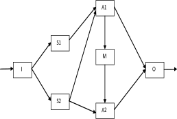
Figure 6: An embedded control system.

7 Case study two: controller design

Here we show how YAGA can be used to provide important diagnostics feedback to a pB developer summarising the failure the EXPECTATIONS clause in a pB machine refinement. We incorporate the key dimensions of systems dependability — availability — the probability that a system resource(s) can be assessed; reliability — the probability that a system meets its stated requirement; safety — expresses that nothing bad happens.

The design in Fig. 6 is originally based on the work by Güdemann and Ortmeier [12]. It consists of two redundant input sensors (S1 and S2) measuring some input signal (I). This signal is then processed in an arithmetic unit to generate the required output signal (O). Two arithmetic units exist, a primary unit (A1) and its backup unit (A2). A1 gets an input signal from both S1 and S2, and A2 only from one of the two sensors. The sensors deliver a signal in finite intervals (but this requirement is not a key design issue since we assume that signals will always be propagated). If A1 produces no output signal, then a monitoring unit (M) switches to A2 for the generation of the output signal. A2 should only produce outputs when it has been triggered by M.

An abstract description of the behaviour of the controller is captured in the specification of Fig. 7. The reliability of the system is given by the real value $rr$; we encode this in the safety specification within the $expectation(.)$ function. State labels $sg=2$ and $sg=3$ denote signal success and failure respectively. Otherwise state labels $sg=0$ and $sg=1$ respectively denote idle state and signal in transit.

$\begin{array}[]{ll}\hline\cr\\ \noindent\mbox{{\bf MACHINE}}&\mbox{SignalTracker ($maxtime,s1p,s2p,a1p,a2p,mp$)}\\ \mbox{{\bf SEES}}&\mbox{Int\_TYPE, Real\_Type}\\ \mbox{{\bf CONSTRAINTS}}&\mbox{$maxtime\in\mathbb{N}\ \wedge\ s1p,s2p,a1p,a2p,mp\in REAL\ \wedge\ s1p,s2p,a1p,a2p,mp:\in real(0)..real(1)$}\\ \mbox{{\bf CONSTANTS}}&\mbox{$rr$}\\ \mbox{{\bf PROPERTIES}}&\mbox{$rr\in REAL\wedge rr\geq real(0)\wedge rr\leq real(1)$}\\ \mbox{{\bf OPERATIONS} }&\\ \quad\quad\mbox{ $sgout\longleftarrow sendsignal\ \ \triangleq\ \ $}&\\ &\mbox{{\bf PRE} $expectation(real(rr))$ {\bf THEN}}\\ &\quad\mbox{{\bf ANY} $sg$ {\bf WHERE} }\\ &\quad\quad\mbox{$sg\geq 0\wedge sg\leq 3\wedge expectation(\textsf{lift}{(sg=0\vee sg=1)}\times real(rr)+\textsf{lift}{(sg=2)})$}\\ &\quad\mbox{\bf THEN}\\ &\quad\quad\mbox{$sgout:=sg$}\\ &\quad\mbox{\bf END;}\\ \mbox{\bf END};\\ \mbox{{\bf END}}&\\ \hline\cr\end{array}$ .

Figure 7: Again we use the $expectation(.)$ function to specify that states where $sg=0(or1)$ are worth the system reliability $rr$; states where $sg=2$ are worth 1 and states where $sg=3$ are worth 0. This encoding is a safety property for the $sendsignal$ operation and must be preserved by any refinement of the abstract machine.

7.1 Refining the controller specification

Here we provide an implementation of the controller by refining the abstract specification in Fig. 7. We also show how to adapt the standard $B$-style modelling of timing constraints [8, 7] to pB models. We use the EXPECTATIONS clause of the form $q\Rrightarrow p\times\textsf{lift}{(s\neq F)}~{}\sqcup~{}\textsf{lift}{\textit{success}}$, which captures the idea that the probability of reaching the “success” state should exceed the given threshold $q$. Here $p$ is a parameter which could vary over the state, but which should initially be at least the value of $q$. Observe that $F$ denotes a state where signal is lost.

But before we do this, we assign individual availability to components of the controller and include the information in the CONSTANTS clause of their abstract machine descriptions. The implementation of the controller as well as the abstract descriptions of its components are in the Appendix. In the next section, we show how to perform dependability analysis on the controller after setting all the components availability to 95% $(s1p=s2p=a1p=a2p=mp=0.95)$. To do this, we use YAGA to provide an equivalent MDP interpretation of the refinement in the PRISM language. This then permits experimental analysis of the refinement and hence generation of system diagnostics to summarise the process.

    ***** Starting Error Reporting  for Failure Traces located on step 6 *****

                Sequence of operations leading to bad state ::>>>
                [{INIT} (1,0,0,0,0,0), {Sensor2Action} (1,0,1,0,0,0),
            {PrimaryAction} (1,0,1,2,0,0), {MonitorAction} (1,0,1,2,0,2),
    {Skip} (1,0,1,2,0,2), {Sensor1Action} (1,2,1,2,0,2), {SendSignal} (3,2,1,2,0,2)]
                    Probability mass of failure trace is:>>>> 0.00012

                Sequence of operations leading to bad state ::>>>
                [{INIT} (1,0,0,0,0,0), {Sensor2Action} (1,0,2,0,0,0),
            {Sensor1Action} (1,1,2,0,0,0), {PrimaryAction} (1,1,2,2,0,0),
    {MonitorAction} (1,1,2,2,0,2), {Skip} (1,1,2,2,0,2), {SendSignal} (3,1,2,2,0,2)]
                    Probability mass of failure trace is:>>>> 0.00012

                Sequence of operations leading to bad state ::>>>
                 [{INIT} (1,0,0,0,0,0), {Sensor2Action} (1,0,1,0,0,0),
            {PrimaryAction} (1,0,1,2,0,0), {MonitorAction} (1,0,1,2,0,2),
    {Skip} (1,0,1,2,0,2), {Sensor1Action} (1,1,1,2,0,2), {SendSignal} (3,1,1,2,0,2)]
                    Probability mass of failure trace is:>>>> 0.00226

            ************ Finished Error Reporting  ... ***************

Figure 8: Diagnostic feedback revealing single traces at endpoint probability distributions (after setting parameter $maxtime=6$) corresponding to the failure of the controller to deliver an output signal. Note that the state tuple in this case is given by ($sg$, $s1$, $s2$, $a1$, $a2$,$m$).

7.2 Experiment 1: identification of critical sets

Step 1:

We set the parameters $q,p:=1$ in the expression $q\Rrightarrow p\times\textsf{lift}{(s\neq F)}~{}\sqcup~{}\textsf{lift}{\textit{success}}$ to identify all failure traces for chosen values of the components availability. Fig. 8 lists three of the failure traces (out of a total of 5) relevant to our discussion, resulting in a maximum probability of failure of 0.0025 after the 6th execution time stamp $i.e.$ $maxtime=6$.

Step 2: From inspection of the above traces we notice that the failure of $A1$ and $M$ enables us to identify them as potential candidates for the construction of our critical set.

Step 3: We verify that their failure will indeed result in overall failure by examining the value of the expectation $\textsf{lift}{(F\land A1\land M)}-\textsf{lift}{(A1\land M)}$.

For candidates such as A1 and M, we use the diagnostic traces to calculate the conditional probabilities as in Def. 6. To do this we extract all the traces which result in $F$ and then examine the variations of the component failures in the traces to identify those which corresponded to a failure configuration.

The results were unsurprising and included for example, identifying that a simultaneous failure of the primary unit $A1$ and the backup monitor $M$. On the other hand, once the $pB$ modelling was completed, the generation of the failure traces was automatic improving the confidence of full coverage. To illustrate this point, a programming mistake was uncovered using this analysis where $A1$ was mistakenly programmed to extract a correct reading only if it received signals from both sensors, rather than from at least $1$.

7.3 Experiment 2: investigating time to failure

This experiment investigates the time to first occurrence of failure given a particular critical set. In fact, the results show that members of the set of interest are indeed critical after verifying their overall conditional probabilities of failure. In summary, for example, a failure tree corresponding to depth $K=6$ yields distributions over endpoints traces whose components time to failure is shown in Table 2.

Identifying critical components time to first failure
Critical Components	Time step to first failure	Maximum probability of failure
S1, S2	2 steps	2.5000 E-3
A1, M	3 steps	2.4938 E-3
A1, A2	4 steps	2.4938 E-3
A1, S2	3 steps	2.4938 E-3

Table 2: Maximum probabilities of failure are computed with respect to endpoint distributions of failure traces (Fig. 8) and conditional probabilities are given by Def. 6.

8 Related work

Traditional approaches for safety analysis via model exploration rely on qualitative assessment — exploring the causal relationship between system subcomponents to determine if some types of failure or accident scenarios are feasible. This is the method largely employed in techniques like the Deductive Cause Consequence Analysis (DCCA) [27], which provides a generalisation of the Fault Tree Analysis (FTA) [20]. Other Industrial methods that support this kind of analysis also include the Failure Modes and Effects Analysis (FMEA) [19] and the Hazard Operability Studies (HAZOP) [9]. But the efficiency of these techniques is largely dependent on the experience of their practitioners. Moreover, with probabilistic systems, where an interplay of random probabilistic updates and nondeterminism characterise system behaviours, such methods are not likely to scale especially with the dependability analysis of industrial sized systems.

The use of probabilistic model-based analysis to explore dependability features in systems construction has recently become a topical issue [22, 11, 12, 4]. One way to achieve this is to use probabilistic counterexamples [13, 5, 6] which can guarantee profiles refuting the desired property i.e. after visiting the reachable states of the supposedly ‘finite’ probabilistic model.

What we have done here is to show how a similar investigation can be achieved for the refinement of proof-based models by taking advantage of the state exploration facility offered by probabilistic model checking. Our method is very precise since it can guarantee the goal of refinement — improving probabilistic results. However, if this does not hold then we are able to provide exact diagnostics summarising the failure provided that computation resources are not scarce.

9 Conclusion and future work

This paper has summarised an approach based on model exploration for the refinement of proof-based probabilistic systems with respect to quantitative safety specifications in the pB language. Our method can provide a pB designer with information necessary to make judgements relating to dependability features of distributed probabilistic systems. We have shown how this can be done for probabilistic loops hence generalising standard models.

Even though most of the failure analysis conjectured herein have been based on intuition, it should be mentioned that a more interesting investigation would be to explore the use of constraint programming techniques to support full coverage of probabilistic system models. This will enable us target larger refinement frameworks as in [10] where probability is not currently being supported.

Acknowledgement: The authors are grateful to Thai Son Hoang for assistance with the pB models of the embedded controller. We also appreciate the anonymous reviewers for their very helpful comments.

$\begin{array}[]{ll}\hline\cr\framebox{{\bf{\Large Appendix}}}&\\ \hline\cr\\ \noindent\par\mbox{{\bf MACHINE}}&\mbox{Clock ($maxtime$) }\\ \mbox{{\bf CONSTRAINTS}}&\mbox{$maxtime\in\mathbb{N}$}\\ \mbox{{\bf VARIABLES}}&\mbox{$time,action$}\\ \mbox{{\bf INVARIANT}}&\mbox{$time\in\mathbb{N}\wedge action\in\mathbb{N}\wedge time\geq 0\wedge time\leq maxtime$}\\ \mbox{{\bf INITIALISATION}}&\mbox{$time,action:=0,0$}\\ \mbox{\bf OPERATIONS}&\\ \quad\quad\mbox{ $timeout\longleftarrow initClock$ \ $\ \triangleq\ $ \ }&\mbox{{\bf BEGIN}}\\ &\quad\quad\quad\mbox{$action:=0\ ||\ timeout:=0$}\\ &\mbox{\bf END;}\\ \quad\quad\mbox{ $timeout\longleftarrow clockAction(label)$ \ $\ \triangleq\ $ \ }&\\ &\mbox{{\bf PRE} $label\in\mathbb{N}\wedge time<maxtime$ {\bf THEN}}\\ &\quad\mbox{{\bf BEGIN}}\\ &\quad\quad\mbox{$action:=label\ ||\ time:=time+1$}\\ &\quad\mbox{\bf END;}\\ &\mbox{\bf END;}\\ &\mbox{$timeout:=time$;}\\ \mbox{{\bf END}}&\\ \\ \hline\cr\end{array}$ .

Figure 9: The specification of the discrete Clock is such that whenever an action due to the components or even a Skip action fires, time is incremented while also marking the specific action. We use the action variable as a marker to abstract the identification of the operations constituting the the diagnostic traces (See Fig. 8).

$\begin{array}[]{ll}\hline\cr\\ \noindent\mbox{{\bf MACHINE}}&\mbox{Cmp ($cp$)}\\ \mbox{{\bf SEES}}&\mbox{Real\_TYPE}\\ \mbox{{\bf CONSTRAINTS}}&\mbox{$cp\in REAL\ \wedge\ cp\geq real(0)\wedge cp\leq real(1)$}\\ \mbox{\bf OPERATIONS}&\\ \\ \quad\quad\mbox{ $cout\longleftarrow componentaction\ \triangleq\ $}&\mbox{{\bf PCHOICE} \ $cp$ \ {\bf OF} }\\ &\quad\quad\mbox{$cout:=1$}\\ &\quad\mbox{{\bf OR}}\\ &\quad\quad\mbox{$cout:=2$}\\ &\quad\mbox{{\bf END;}}\\ \mbox{{\bf END}}&\\ \\ \hline\cr\end{array}$ .

Figure 10: Here we model an abstract stateless machine for components with similar behaviours. Later on, we shall use pB’s IMPORT clause to clone Sensor1, Sensor2, PrimaryUnit, Monitor and Backup Units via variable renaming. The specification of the abstract Cmp machine is such that it can probabilistically either respond to a signal request $(cout=1[active])$ or it fails to do so $(cout=2[dead])$ . The probability $cp$ is a paremeter of the machine and specifies the availability of the component.

$\begin{array}[]{ll}\hline\cr\noindent\par\mbox{{\bf MACHINE}}&\mbox{SignalProcess($s1p,s2p,a1p,a2p,mp$)}\\ \mbox{{\bf CONSTRAINTS}}&\mbox{$s1p,s2p,a1p,a2p,mp\in REAL\ \wedge\ s1p,s2p,a1p,a2p,mp:\in real(0)..real(1)$}\\ \mbox{{\bf INCLUDES}}&\mbox{Sensor1.Cmp(s1p), Sensor2.Cmp(s2p), PrimaryUnit.Cmp(a1p),}\\ &\mbox{BackupUnit.Cmp(a2p), Monitor.Cmp(mp)}\\ \mbox{{\bf VARIABLES}}&\mbox{$s1,s2,a1,a2,m$}\\ \mbox{{\bf INVARIANT}}&\mbox{$s1,s2,a1,a2,m\in\mathbb{N}\wedge s1,s2,a1,a2,m::[0,2]$}\\ \mbox{{\bf INITIALISATION}}&\mbox{$s1,s2,a1,a2,m:=0$}\\ \mbox{\bf OPERATIONS}&\\ \quad\quad\mbox{ $label\longleftarrow action\ \triangleq\ $ }&\\ &\quad\mbox{{\bf SELECT} $s1=0$ {\bf THEN}}\\ &\quad\quad\mbox{$s1\longleftarrow Sensor1.componentaction\ ||\ label:=1$}\\ &\quad\mbox{{\bf WHEN} $s2=0$ {\bf THEN}}\\ &\quad\quad\mbox{$s2\longleftarrow Sensor2.componentaction\ ||\ label:=2$}\\ &\quad\mbox{{\bf WHEN} $a1=0\wedge s1=1$ {\bf THEN} }\\ &\quad\quad\mbox{$a1\longleftarrow PrimaryUnit.componentaction\ ||\ label:=3$}\\ &\quad\mbox{{\bf WHEN} $a1=0\wedge s2=1$ {\bf THEN} }\\ &\quad\quad\mbox{$a1\longleftarrow PrimaryUnit.componentaction\ ||\ label:=3$}\\ &\quad\mbox{{\bf WHEN} $a1=2$ {\bf THEN}}\\ &\quad\quad\mbox{$m\longleftarrow Monitor.componentaction\ ||\ label:=4$}\\ &\quad\mbox{{\bf WHEN} $m=1$ {\bf THEN}}\\ &\quad\quad\mbox{$a2\longleftarrow BackupUnit.componentaction\ ||\ label:=5$}\\ &\quad\mbox{{\bf ELSE} $label:=6$}\\ \\ \quad\quad\mbox{ $s1out,s2out,a1out,a2out,mout\longleftarrow getState\ \triangleq\ $}&\mbox{ {\bf BEGIN} s1out,s2out,a1out,a2out,mout := s1,s2,a1,a2,m {\bf END};}\\ \mbox{{\bf END}}&\\ \hline\cr\end{array}$
.

Figure 11: The nondeterministic behaviour of the components is specified in this machine. An individual component can probabilistically respond to a signal request by setting its state value to 1 or 2 denoting ‘active’ and ‘dead’ respectively, after leaving the initial state with value 0 (’idle’).

$\begin{array}[]{ll}\hline\cr\\ \noindent\mbox{{\bf IMPLEMENTATION}}&\mbox{SignalTrackerI($maxtime,s1p,s2p,a1p,a2p,mp$)}\\ \mbox{{\bf REFINES}}&\mbox{SignalTracker}\\ \mbox{{\bf SEES}}&\mbox{Real\_TYPE, Int\_TYPE}\\ \mbox{{\bf IMPORTS}}&\mbox{SignalProcess($s1p,s2p,a1p,a2p,mp$), Clock($maxtime$)}\\ \mbox{\bf OPERATIONS}&\\ \quad\quad\mbox{$sgout\longleftarrow sendsignal$ \ $\ \triangleq\ $ \ }&{\bf VAR}\ $sg, s1, s2, a1, a2, m, t$\ {\bf IN}\\ \quad\quad\quad\quad\mbox{{}}&\mbox{$t\leftarrow initClock$;}\\ \\ &\mbox{{\bf WHILE} ($t\leq maxtime$) {\bf DO}}\\ &\quad\quad\mbox{$act\longleftarrow action;t\leftarrow clockAction(act);$ }\\ &\quad\quad\mbox{$s1,s2,a1,a2,m\longleftarrow getState$; }\\ \\ &\quad\mbox{{\bf IF} $(a2=1)\wedge(s2=1)$ {\bf THEN} }\\ &\quad\quad\quad\mbox{$sg:=2$;}\\ &\quad\mbox{{\bf ELSIF} $(a1=1)\wedge(s1=1)$ {\bf THEN} }\\ &\quad\quad\quad\mbox{$sg:=2$};\\ &\quad\mbox{{\bf ELSIF} $(a1=1)\wedge(s2=1)$ {\bf THEN} }\\ &\quad\quad\quad\mbox{$sg:=2$};\\ &\quad\mbox{{\bf ELSE}}\\ &\quad\quad\quad\mbox{$sg:=3$};\\ &\mbox{{\bf END;}}\\ &\quad\quad\quad\mbox{$sgout:=sg$;}\\ &\mbox{{\bf INVARIANT} {\quad$s1,s2,a1,a2,m,t\ \in\mathbb{N}\ \wedge s1,s2,a1,a2,m::[1,2]\wedge sg::[0,3]\ \wedge\ t\leq maxtime$}}\\ &\mbox{{\bf EXPECTATIONS} \quad$real(rr)\Rrightarrow$ ({{lift}{$(sg=0\vee sg=1)$} $\times real(rr)$ {+ {lift}{$(sg=2))$}} $\times$ {lift}{$(t=maxtime)$}}}\\ \mbox{{\bf END;}}\\ \mbox{{\bf END}}&\\ \hline\cr\end{array}$ .

Figure 12: SignalTrackerI uses a WHILE-DO loop structure to model the passage of discrete time. The PCHOICE operation provides implementation constructs of the abstract probabilistic branching statements with respect to the availability of the controller components.

References

- [1]
- [2] J. R. Abrial (1996): The B-Book: Assigning programs to meaning. Cambridge University Press.
- [3] J. R. Abrial (2009): Modeling in Event-B: system and software engineering. To appear. Cambridge University Press. Available at http://www.event-b.org.
- [4] H. Aljazzar, M. Fischer, L. Grunske, M. Kuntz, F. Leitner & S. Leue (2009): Safety analysis of an airbag system using probabilistic FMEA and probabilistic counterexamples. In proceedings of QEST’09, pp. 299–308, 10.1109/QEST.2009.8.
- [5] H. Aljazzar & S. Leue (2009): Generation of counterexamples for model checking of Markov Decision Processes. In proceedings of QEST’09, pp. 197–206, 10.1109/QEST.2009.10.
- [6] M. E. Andrs, P. D’ Argenio & P. v Rossum (2009): Significant diagnostic counterexamples in probabilistic model checking. In proceedings of HVC’08. Lecture Notes in Computer Science 5394, pp. 129–148, 10.1007/978-3-642-01702-5_15.
- [7] M. Butler (2009): Using Event-B refinement to verify a control strategy. Technical Report, University of Southampton, United Kingdom.
- [8] D. Cansell, D. Mry & J. Rehm (2006): Time constraint patterns for Event-B development. In proceedings of B’07. Lecture Notes in Computer Science 4355. Springer, pp. 140–154, 10.1007/11955757_13.
- [9] Chemical Industries Association Limited, London (1987): CIA.: A guide to hazard and operability studies.
- [10] : Deploy. Available at http://www.deploy-project.eu/.
- [11] L. Grunske, R. Colvin & K. Winter (2007): Probabilistic model checking support for FMEA. In proceedings of QEST’07, 10.1109/QEST.2007.18.
- [12] M. Gudemann & F. Ortmeier (2010): Probabilistic model-based safety analysis. In proceedings of QAPL’10. EPTCS 28, pp. 114–128, 10.4204/EPTCS.28.8.
- [13] T. Han, J.-P Katoen & B. Damman (2009): Counterexamples generation in probabilistic model checking. IEEE Transaction on software engineering 32(2), pp. 241–257, 10.1007/978-3-540-71209-1_8.
- [14] H. Hansson & B. Jonsson (1994): A logic for reasoning about time and reliability. Formal Aspects of Computing 6(5), pp. 512–535, 10.1007/BF01211866.
- [15] A. Hinton, M. Kwiatkowska, G. Norman & D. Parker (2006): PRISM: A tool for automatic verification of probabilistic systems. In proceedings of TACAS’06. Lecture Notes in Computer Science 3920. Springer, pp. 441–444, 10.1007/11691372_29.
- [16] T. S. Hoang (2005): Developing a probabilistic B-Method and a supporting toolkit. Ph.D. thesis, University of New South Wales, Australia.
- [17] C. A. R. Hoare (1969): An axiomatic basis for computer programming. Communications of the ACM 12(10), pp. 576–580, 10.1145/357980.358001.
- [18] J. Hurd (2002): Formal verification of probabilistic algorithms. Ph.D. thesis, University of Cambridge, United Kingdom.
- [19] Internatinal Electrotechnical Commission, Geneva (1985): IEC International Standard 812: “Analysis techniques for system reliability: procedures for failure mode and effect analysis.
- [20] Internatinal Electrotechnical Commission, Geneva (1990): International Standard IEC 1025: Fault Tree Analysis (FTA).
- [21] D.R. Karger (1993): Global min-cuts in RNC, and other ramifications of a simple min-out algorithm. In proceedings of fourth annual ACM-SIAM symposium on discrete algorithms. pp 21-30, Austin, Texas, United States.
- [22] M. Kwiatkowska, G. Norman & D. Parker (2007): Controller dependability analysis by probabilistic model checking. Control Engineering Practice 15(11), pp. 1427–1434, 10.1016/j.conengprac.2006.07.003.
- [23] A.K. McIver & C.C. Morgan (2004): Abstraction, refinement and proof for probabilistic systems. Monographs in Computer Science. Springer Verlag.
- [24] U. Ndukwu (2009): Quantitative safety: linking proof-based verification with model checking for probabilistic systems. In proceedings of QFM’09. EPTCS 13, pp. 27–39, 10.4204/EPTCS.13.3.
- [25] U. Ndukwu (2010): Generating counterexamples for quantitative safety specifications in probabilistic B. Accepted for inclusion in the journal of logic and algebraic programming.
- [26] U. Ndukwu & A.K. McIver (2010): YAGA: Automated analysis of quantitative safety specifications in probabilistic B. In proceedings of ATVA’10. Lecture Notes in Computer Science 6252. Springer, pp. 378–386, 10.1007/978-3-642-15643-4_31.
- [27] F. Ortmeier, W. Reif & G. Schellhorn (2006): Deductive cause-consequence analysis (DCCA). In proceedings of IFAC World Congress, Elsevier.
- [28] M.L. Puterman (1994): Markov Decision Processes. Wiley.
.
.
.
.