Inducing odd-frequency triplet superconducting correlations in a normal metal

Abstract

This work discusses theoretically the interplay between the superconducting and ferromagnetic proximity effects, in a diffusive normal metal strip in contact with a superconductor and a non-uniformly magnetized ferromagnetic insulator. The quasiparticle density of states of the normal metal shows clear qualitative signatures of triplet correlations with spin one (TCS1). When one goes away from the superconducting contact, TCS1 focus at zero energy under the form of a peak surrounded by dips, which show a typical spatial scaling behavior. This effect can coexist with a focusing of singlet correlations and triplet correlations with spin zero at finite but subgap energies. The simultaneous observation of both effects would enable an unambigous characterization of TCS1.

Hybrid superconducting/ferromagnetic circuits allow to obtain fascinating unconventional superconducting correlationsRevueBuzdin . Although a standard s-wave superconductor naturally hosts even-frequency superconducting correlations, the superconducting proximity effect in an adjacent ferromagnet can lead to odd-frequency pairing, because the ferromagnetic exchange field lifts time reversal symmetry. This can correspond to either triplet superconducting correlations with spin zero (TCS0), i.e. correlations between opposite electronic spins, or triplet superconducting correlations with spin one (TCS1), i.e. correlations between equal spins. The existence of TCS0 is confirmed experimentally since a decade (see e.g. KontosDOS ; Ryazanov ; KontosI ). The possibility of obtaining TCS1 has been investigated more recentlyRevueBergeret . The features observed so far are quantitative. It has been observed that, in certain conditions, ferromagnets can sustain a supercurrent on a much longer lengthscale than expectedKeizer . This suggests the presence of TCS1, because in diffusive ferromagnets, TCS1 are expected to propagate on a much longer distance than TCS0Eschrig . Most of the strategies discussed so far to observe TCS1 require to measure a supercurrent, which is an energy-integrated quantity. Alternatively, the quasiparticle density of states (DOS) yields spectroscopic information and thus appears as a powerful tool to characterize the nature of superconducting correlations. This paper presents a geometry in which the DOS gives a particularly rich access to odd-frequency superconducting correlations.

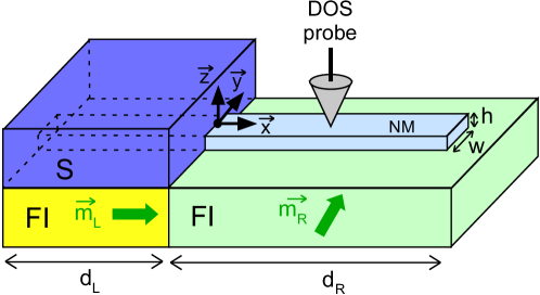
Figure 1: Scheme of the lateral geometry considered in this work (see text).

I suggest to use a lateral geometry, where the superconducting correlations are induced in a normal metal (NM) strip in contact with a superconductor (S) and a ferromagnetic insulator (FI) with two non-colinear magnetization domains. This configuration is compatible with spatially resolved DOS measurements using several tunnel contact probesGueron or a low temperature STMLe Sueur . The propagation of odd-frequency superconducting correlations has been studied thoroughly in ferromagnetsRevueBergeret , but only elusively in NMsAsano ; Yokoyama ; Yokoyama3 . Here, the FI turns the NM strip into an effective ferromagnet with an unusually weak exchange field. This is advantageous to study the propagation of odd-frequency superconducting correlations. The TCS1 induce a zero-energy peak in the DOS of the NMAsano . Such an effect is not specific to TCS1Fauchere ; Krawiec ; Linder2 ; Yokoyama2 . However, in the present geometry, important additional features allow to identity unambiguously TCS1. Indeed, the low-energy DOS peak is surrounded by dips, and this structure shows a characteristic spatial scaling behavior when one goes away from the superconducting contact, i.e. it ”shrinks” on a lenghtscale which depends on a longitudinal Thouless energy. If one observes simultaneously finite energy dips, which confirm the existence of the effective exchange field inside the NM, the zero-energy peak points unambiguously to TCS1.

I consider the lateral geometry of Fig.1, where the central element is a NM strip with thickness $h$, width $w$, and longitudinal coordinate $x$. A portion with length $d_{L}$ of the NM strip is contacted to a S and a FI domain magnetized along a direction $\vec{m}_{L}$ for $x<0$, and a portion with length $d_{R}$ is contacted to a FI domain magnetized along a direction $\vec{m}_{R}$ for $x>0$. I assume that the structure is diffusive, so that a quasiclassical isotropic Green’s function $G$ can be used to describe the propagation of superconducting correlations inside the NMconventions . The function $G$ has a structure in the spin and Nambu (electron-hole) subspaces, so that it can be decomposed in terms of the spin[Nambu] Pauli matrices $\sigma_{i}$[$\tau_{i}$] (see below). In the following, I use $\vec{m}_{L}=\vec{x}$. In the colinear case $\vec{m}_{R}=\vec{x}$, only singlet correlations and TCS0 can appear inside the NM. In the non-colinear case $\vec{m}_{R}\neq\vec{x}$, TCS1 can also appear.

The spatial evolution of $G$ inside the NM is described by the Usadel equation $\hbar D\rho\vec{\nabla}\mathbf{.}\vec{j}=-(i\varepsilon-\Gamma)\left[\check{\tau}_{3},G\right]$, with $\rho$ the resistivity of the NMUsadel . The density of matrix current $\vec{j}=G\vec{\nabla}G/\rho$ characterizes the flows of charge, spin and electron-hole coherence in the device. The rate $\Gamma$ accounts for inelastic processes. The Usadel equation alone is not sufficient to predict the behavior of $G$, because the influence of the $S$ and $FI$ contacts must be taken into account. When $h$ and $w$ are smaller than the typical spatial scale $\xi$ characterizing the variations of $G$ inside the NMxi , it is possible to derive a one-dimensional effective Usadel equation on $G\simeq G(x)$, which takes into account the effects of the S and FI contacts. This equation can be derived with an approach inspired from circuit theoryCircuitTheory , using spin dependent boundary conditions for isotropic Green’s functionsBCIGF . This requires to define a surface tunnel conductance $G_{T}^{s}$ for the S/NM interface and a surface conductance-like coefficient $G_{\phi}^{s}$ for the NM/FI interface. The last parameter accounts for the fact that electrons from the NM are reflected by the FI with spin-dependent reflection phases. Indeed, the internal Stoner exchange field of the FI can affect the evanescent tails of electronic wavefunctions on a scale of a few atomic layers. One finds, for $x<0$

$$2l^{2}\mathbf{\nabla}_{x}(G\mathbf{\nabla}_{x}G)=-2\gamma_{\varepsilon}\left[\check{\tau}_{3},G\right]-\gamma_{T}\left[G,G_{S}\right]+i\gamma_{\phi}[\tau_{3}\sigma_{L},G]$$ (1)

with $E_{Th}=\hbar D/h^{2}$, $\gamma_{\varepsilon}=(i\varepsilon-\Gamma)/E_{Th},\gamma_{T}=G_{T}^{s}\rho h$, $\gamma_{\phi}=G_{\phi}^{s}\rho h$ and $\sigma_{L(R)}=\vec{m}_{L(R)}.\vec{\sigma}$. Here, $G_{S}$ denotes the value of the isotropic Green’s function inside the superconductor. For $x>0$, one finds a similar equation with $\gamma_{T}$ replaced by $0$ and $\sigma_{L}$ by $\sigma_{R}$.

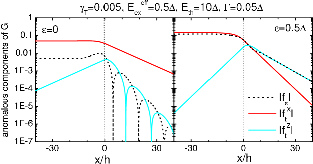
Figure 2: Absolute values of the anomalous components $f_{s}$, $f_{t}^{x}$ and $f_{t}^{z}$ of $G$ in the NM strip at $\epsilon=0$ (left panel) and $\epsilon=E_{ex}^{eff}$ (right panel) respectively, for $\vec{m}_{R}=\vec{z}$ and $d_{L(R)}\longrightarrow+\infty$.

Equation (1) describes an interplay between the superconducting and ferromagnetic proximity effects. On the one hand, the $\gamma_{T}$ terms tend to induce a minigap inside the NM, due to the confinement of electrons in the $\vec{z}$ direction. This effect depends on the interface parameter $\gamma_{T}\$but also the lateral Thouless energy $E_{Th}$ defined below Eq. (1). For instance, at the left end of the NM strip, the DOS is suppressed for energies $\left|\varepsilon\right|<\tilde{\Delta}=E_{Th}\gamma_{T}/2$ when $d_{L}\rightarrow+\infty$, $E_{Th}\gamma_{T}\ll\Delta$ and $\gamma_{\phi}=0$. On the other hand, the interface parameter $G_{\phi}^{s}$ causes an effective exchange field $E_{ex}^{eff}=E_{Th}\gamma_{\phi}/2=\hbar DG_{\phi}^{s}\rho/h$ oriented along $\vec{x}$ [$\vec{m}_{R}$] at the left[right] side of the NM strip, i.e. $x<0$ [$x>0$] Huertas-Hernando . This type of effective field has already been observed and accurately characterized for various types of S/FI bilayersTedrow ; Hao ; Meservey ; Xiong . For $x<0$, the exchange field due to the left contact splits the minigap induced by the S contact and induces TCS0 with respect to the $\vec{x}$ direction. These correlations can propagate to the right part of the NM strip where they correspond to TCS1 when $\vec{m}_{R}=\vec{z}$. The induction of TCS1 in diffusive S/F structures present similarities with this processRevueBergeret . However, minigap effects are usually destroyed in ferromagnets, due to strong ferromagnetic exchange fields, except in some particular disordered casesIvanov . Besides, $E_{ex}^{eff}$ is expected to be much smaller than the exchange field inside standard ferromagnets. Hence, the situation studied here is qualitatively different from that of standard S/F structures. Interestingly, for a given type of NM/FI contact, the amplitude of $E_{ex}^{eff}$ can be tuned by choosing $h$ at the sample fabrication stage, since $E_{ex}^{eff}$ scales with $1/h$ Hao ; Huertas-Hernando ; Cottet . This gives an interesting flexibility with respect to material constraints.

In the following, I assume that the value $G_{S}$ of $G$ inside the superconductor is equal to the bulk BCS value, i.e. $G_{S}=\cos(\theta_{S})\check{\tau}_{3}+\sin(\theta_{S})\check{\tau}_{1}$, with $\theta_{S}=\arctan[\Delta/(-i\varepsilon+\Gamma)]$. Inside the NM, one can use the angular parametrization $G=\tau_{3}(\cosh\eta)\cos(\theta)+i\sinh(\eta)\sin(\theta)\vec{v}.\vec{\sigma})$+$\tau_{1}(f_{s}+\vec{f}_{t}.\vec{\sigma})$, with $f_{s}=\cosh(\eta)\sin(\theta)$, $\vec{f}_{t}=-i\sinh(\eta)\cos(\theta)\vec{v}$, and $\vec{v}$ a unit vector. This convention automatically satisfies the normalization condition $G^{2}=1$. I discuss below the anomalous components of $G$, i.e. $f_{s}$, $f_{t}^{x}=\vec{f}_{t}.\vec{x}$ and $f_{t}^{z}=\vec{f}_{t}.\vec{z}$, which reveal the existence of superconducting correlations inside the NM. Defining TCS0 and TCS1 components requires to define a reference direction $\vec{m}_{ref}$. A natural choice is to use $\vec{m}_{ref}=\vec{m}_{L}$ for $x<0$ and $\vec{m}_{ref}=\vec{m}_{R}$ for $x>0$. Then, TCS0 and TCS1 correspond to the components of $\vec{f}_{t}$ parallel and perpendicular to $\vec{m}_{ref}$, respectively. The DOS inside the strip can be calculated as $N(\varepsilon)/N_{0}={\textstyle\sum\nolimits_{\sigma}}\operatorname{Re}[\cos(\theta+i\sigma\eta)]/2$, with $N_{0}$ the normal state DOS of the NM.

The spatial evolution of the DOS can be first studied with an analytic linearized description, which yields a transparent interpretation of the circuit behavior. This approach is valid in the limit of a weak superconducting proximity effect, i.e. $\theta,\eta\ll 1$ inside the NM. This occurs e.g. when $\gamma_{T}$ is small and $\Gamma$ large, so that the minigap is closed and just gives residual dips at the left side of the NM strip. For simplicity, I assume $d_{L(R)}\longrightarrow+\infty$. For $x<0$ one has

$$[f_{s},f_{t}^{x},f_{t}^{z}]=[0,0,1]A_{0}e^{k_{S}x}+{\displaystyle\sum\limits_{\sigma=\pm 1}}[1,\sigma,0]\left(\frac{\Theta_{\sigma}^{B}}{2}+A_{\sigma}e^{-\tilde{k}_{\sigma}x}\right)$$ (2)

with $k_{S}^{2}h^{2}-\gamma_{T}\cos(\theta_{S})=-2i[(\varepsilon+i\Gamma)/E_{Th}]$, and $\tilde{k}_{\sigma}h^{2}-\gamma_{T}\cos(\theta_{S})=2i[\sigma E_{ex}^{eff}-\varepsilon-i\Gamma]/E_{Th}$. Here, I note

$$\Theta_{\sigma}^{B}=\arctan[\frac{\gamma_{T}\sin\left[\theta_{S}\right]}{\gamma_{T}\cos\left[\theta_{S}\right]+2[-i\epsilon+\Gamma+i\sigma E_{ex}^{eff}]/E_{Th}}]$$ (3)

the value of $\theta-i\eta\sigma$ at $x\rightarrow-\infty$. For $x>0$ and $\vec{m}_{R}=\vec{z}$, one has

$$[f_{s},f_{t}^{x},f_{t}^{z}]=[0,1,0]B_{0}e^{-k_{0}x}+{\displaystyle\sum\limits_{\sigma=\pm 1}}[1,0,\sigma]B_{\sigma}e^{-k_{\sigma}x}$$ (4)

with $k_{0}^{2}h^{2}=-2i[(\varepsilon+i\Gamma)/E_{Th}]$ and $k_{\sigma}h^{2}=2i[\sigma E_{ex}^{eff}-\varepsilon-i\Gamma]/E_{Th}$. For $x>0$ and $\vec{m}_{R}=\vec{x}$, the second and third components of the vectors in Eq.(4) must be exchanged. The coefficients $A_{\sigma}$, $A_{0}$, $B_{\sigma}$, and $B_{0}$ can be calculated by assuming the continuity of $f_{s},f_{t}^{x},f_{t}^{z}$ and their first derivatives at $x=0$. This leads to the results shown in Fig. 2, obtained for $\vec{m}_{R}=\vec{z}$ (non-colinear case).

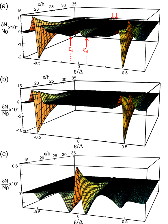
Figure 3: Density of states in the NM in the non-colinear case $\vec{m}_{R}=\vec{z}$ (panel a), the colinear case $\vec{m}_{R}=\vec{x}$ (panel b), and the case where there is no FI contact at $x>0$ (panel c). The data are shown in terms of the deviation $\delta N=N-N_{0}$ of the DOS in the NM from the normal state value $N_{0}$. The parameters used are the same as in Fig. 2.

At zero-energy and $x\rightarrow-\infty$, $f_{t}^{x}$ is dominant due to $\gamma_{T}\ll\gamma_{\phi}$ (Fig. 2, left panel)Linder1 . I now comment the behavior of the different types of correlations for $x>0$ (Fig. 2, right panel). In this area, TCS1 ($f_{t}^{x}$) propagate independently of the two other components, with the characteristic vector $k_{0}$. At $\varepsilon=0$, $k_{0}$ is small, so that TCS1 propagate on a relatively long distance: this is why TCS1 are usually called ”long-range” correlations. However, this is true only at low energies. Indeed, for $\varepsilon=\pm E_{ex}^{eff}$,  the real part of $k_{0}$ is larger, so that TCS1 decay more quickly. Conversely, for $x>0$ and $\varepsilon=0$, the propagation of singlet correlations ($f_{s}$) and TCS0 ($f_{t}^{z}$) is short-range. Indeed, $f_{s}$ and $f_{t}^{z}$ show a damped oscillatory behavior ruled by the propagation vectors $k_{\sigma}$, which correspond to a scale $(\hbar D/E_{ex}^{eff})^{1/2}$ for $E_{ex}^{eff}\gg\Gamma$ and $\varepsilon=0$. In contrast, for $\varepsilon=\pm E_{ex}^{eff}$, the $f_{s}$ and $f_{t}^{z}$ components do not oscillate and decay more slowly. Hence, it is the singlet correlations and TCS0 which are long-range for $\varepsilon=\pm E_{ex}^{eff}$. As a result, sufficiently far from the superconductor, TCS1 become dominant at $\varepsilon=0$, whereas singlet correlations and TCS0 become dominant for  $\varepsilon=\pm E_{ex}^{eff}$. In other terms, one obtains $\vec{v}(\varepsilon=0)\simeq\vec{x}$ and $\vec{v}(\varepsilon=\pm E_{ex}^{eff})\simeq\vec{z}$. This leads to characteristic features in the energy dependence of the DOS, shown by Fig. 3a. For $x$ sufficiently large, one obtains characteristic dips at $\varepsilon\simeq\pm E_{ex}^{eff}$, due to singlet correlations and TCS0. In contrast, TCS1 produce a zero-energy peak which reaches a maximum higher than the normal-state DOS $N_{0}$. Importantly, $N(0)>N_{0}$ is not specific to TCS1. Indeed, an enhanced zero-energy DOS can also be due for instance to interaction effectsFauchere , or to TCS0Buzdin ; Linder1 ; Linder2 ; Yokoyama2 , as observed experimentally in S/F bilayersKontosDOS . However, in the present geometry, TCS1 can be detected unambiguously due to the additional features discussed below.

Due to the peculiar energy dependence of $k_{0}$, the zero-energy DOS peak is surrounded by low-energy dips, and this ensemble shows a characteristic spatial scaling behavior when $x$ increases (see Fig. 3a). Let us note $\pm\varepsilon_{d}$ the position of the low-energy dips. In the limit of a vanishing $\Gamma$, $\varepsilon_{d}$ scales with a longitudinal Thouless energy $\tilde{E}_{Th}=\hbar D/x^{2}$, provided the finite energy dips are well separated from the low-energy peak, i.e. $\varepsilon_{d}\ll E_{ex}^{eff}$. When $\Gamma$ is finite, a scaling behavior can persist. For instance, in the limit $\varepsilon_{d}\ll\Gamma,E_{ex}^{eff}$, Eq. (4) gives

$$\varepsilon_{d}\simeq\pi\sqrt{\Gamma\tilde{E}_{Th}/2}\varpropto 1/x$$ (5)

The scaling behavior of the low energy DOS features represents a ”smoking-gun” for the fact that some superconducting correlations propagate along the strip with the vector $k_{0}$. Importantly, the DOS dips at $\varepsilon\simeq\pm E_{ex}^{eff}$ follow an equivalent scaling behavior, due to the structure of the $k_{\sigma}$ vectors. It is instructive to discuss other magnetic configurations. Figure 3.b shows the DOS of the NM in the colinear case. The finite energy dips are still present, but there is no low-energy features because TCS1 are absent. At last, Fig 3c. shows the DOS of the NM when there is a FI contact with a uniform magnetization at $x<0$, but no FI contact or $E_{ex}^{eff}=0$ at $x>0$. In this case, for $x>0$, weak DOS dips appear at $\varepsilon\simeq\pm E_{ex}^{eff}$, due to the spin-split minigap effect occurring for $x<0$. Importantly, these dips are very different from those obtained in the previous cases: they are not surrounded by peaks and quickly vanish with increasing $x$. In contrast, there is still a spatially-scaling zero-energy peak, although there is no TCS1 in the circuit. This is because singlet correlations and TCS0 propagate with the characteristic vector $k_{0}$ in this case. One can conclude that it is important to see DOS dips appear at $\varepsilon\simeq\pm E_{ex}^{eff}$ and persist with increasing $x$, to confirm the existence of $E_{ex}^{eff}$ at the right side of the strip. In this case, the spatially-scaling zero-energy peak can only be due to TCS1, which is the only component which can propagate with $k_{0}$. For a good visibility of the finite-energy DOS dips, it is important to use $E_{ex}^{eff}<\Delta$. In practice, this limit can be reached by using an appropriate value for $h$. Note that the long-range behavior of TCS0 and singlet correlations at $\varepsilon=\pm E_{ex}^{eff}$ is usually not discussed for standard ferromagnets, in which exchange fields are too high.

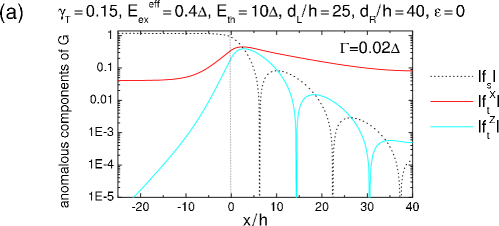
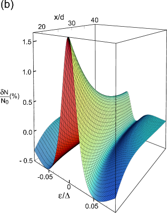
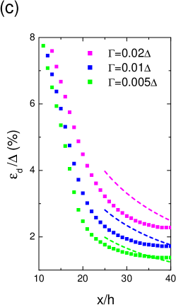
Figure 4: Predictions for $\vec{m}_{R}=\vec{z}$, a value of $\gamma_{T}$ much larger than in Figs. 2 and 3, and finite values of $d_{L(R)}$. Panel a shows $\left|f_{s}\right|$, $\left|f_{t}^{x}\right|$ and $\left|f_{t}^{z}\right|$ at zero energy, as a function of the coordinate $x$. Panel b shows $\delta N$ as a function of $\varepsilon$ and $x$. Panel c shows the dependence of $\varepsilon_{d}$ on $x$, for various values of $\Gamma$. The value $\Gamma=0.02\Delta$ is used in panels a and b. All curves have been obtained with the numerical approach, except the dotted lines in panel c, which correspond to Eq.(5).

The amplitude of the DOS variations in Figs. 2 and 3 is very weak due to the small $\gamma_{T}$ used. Experimental observations call for an increase in $\gamma_{T}$. This requires to use a numerical approach to solve the problem in the non-linear limit. In practice, ferromagnetic domains have a finite size, so that $d_{L}$ and $d_{R}$ must be finite. The resulting finite size effects are studied below with the numerical approach. Figure 4 presents results for the non-colinear case. The spatial behaviors of $f_{t}^{x}$, $f_{t}^{z}$ and $f_{s}$ remain qualitatively similar (see Fig 4.a). At $x>0$, $f_{t}^{x}$ still yields the expected low-energy features in the DOS (Fig.4b). The variations of $\varepsilon_{d}$ with $x$ are shown in Fig.4c for various values of $\Gamma$ (symbols). The scaling behavior of the DOS low-energy features is robust to finite size effects. One can check that the semi-infinite expression Eq. (5) yields the right order of magnitude for $\varepsilon_{d}$ at the right boundary of the NM strip. Finite size effects slow down the scaling behavior of the low-energy features at $x\longrightarrow d_{R}$, i.e. one has $\partial\varepsilon_{d}/\partial x\longrightarrow 0$. Nevertheless, it is still possible to observe a strong decrease of $\varepsilon_{d}$ with $x$, when $x$ is not too close to $d_{R}$. If $\gamma_{T}$ is too large with respect to $\gamma_{\phi}$, the zero-energy DOS peak has a reduced amplitude because $f_{t}^{x}$ is weakLinder1 . To maximize $N(0)$, one must use $\gamma_{T}=\gamma_{\phi}$ and decrease $\Gamma$. For instance, using $\gamma_{T}=0.08$, $\Gamma=0.005\Delta$ and the other parameters of Fig.4.b (in particular, $\gamma_{\phi}=0.08$), one obtains $N(0)=1.35N_{0}$ at $x=40h$. Nevertheless, using unfavorable parameters like those of Fig.4.b, one still obtains $N(0)=1.00325N_{0}$ at $x=40h$, and amplitude which is measurable, in principleKontosDOS . The geometry discussed here also presents the advantage that spin-flip scattering effects, which could reduce the amplitude of odd-frequency superconducting correlations, are usually small in NMs. Interestingly, a NM strip with a S contact but no ferromagnetic contacts has been studied experimentally ($E_{ex}^{eff}=0$ for any $x$). In this case, one can only have singlet correlations propagating with $k_{0}$. As a result, a spatially-scaling zero-energy dip has been observed in the DOS of the NMGueron ; BelzigTM .

To conclude, TCS1 can appear in a diffusive NM strip in contact with a S and a FI with several non-colinear magnetic domains. These correlations induce in the DOS of the NM a low-energy peak surrounded by dips, which show a characteristic spatial scaling behavior away from the S contact. Meanwhile, if the thickness of the strip is chosen properly, superconducting correlations between opposite spins will focus at finite but subgap energies. The simultaneous observation of both effects would enable an unambiguous identification of TCS1.

I thank T. Kontos and W. Belzig for useful discussions.

References

- (1) A. I. Buzdin, Rev. Mod. Phys. 77, 935 (2005).
- (2) T. Kontos et al., Phys. Rev. Lett. 86, 304 (2001).
- (3) V. V. Ryazanov et al., Phys. Rev. Lett. 86, 2427 (2001).
- (4) T. Kontos, et al., Phys. Rev. Lett. 89, 137007 (2002).
- (5) F. S. Bergeret et al., Rev. Mod. Phys. 77, 1321 (2005).
- (6) R. S. Keizer, et al., Nature (London) 439, 825 (2006); T.S. Khaire et al., Phys. Rev. Lett. 104, 137002 (2010); J. W. A. Robinson et al., Science 329, 59 (2010); D. Sprungmann et al., Phys. Rev. B 82, 060505 (2010).
- (7) M. Eschrig and T. Lofwander, Nature Physics 4, 138 (2008); M. Houzet and A. I. Buzdin, Phys. Rev. B 76, 060504(R) (2007); A. F. Volkov and K. B. Efetov, Phys. Rev. B 81, 144522 (2010); J. Linder and A. Sudbø, Phys. Rev. B 82, 020512(R) (2010).
- (8) S. Guéron et al., Phys. Rev. Lett. 77, 3025 (1996).
- (9) H. Le Sueur et al., Phys. Rev. Lett. 100, 197002 (2008).
- (10) Y. Asano, Phys. Rev. Lett. 98, 107002 (2007); V. Braude and Yu. V. Nazarov, Phys. Rev. Lett. 98, 077003 (2007).
- (11) T. Yokoyama, and Y. Tserkovnyak, Phys. Rev. B 80, (2009).
- (12) T. Yokoyama et al., Phys. Rev. Lett. 106, 246601 (2011).
- (13) A. L. Fauchère et al., Phys. Rev. Lett. 82, 3336 (1999).
- (14) M. Krawiec et al., Phys. Rev. B 70, 134519 (2004).
- (15) J. Linder et al., Phys. Rev. B 81, 214504 (2010).
- (16) T. Yokoyama et al., Phys. Rev. B 75, 134510 (2007).
- (17) A. Buzdin, Phys. Rev. B 62, 11377 (2000).
- (18) J. Linder et al., Phys. Rev. Lett. 102, 107008 (2009).
- (19) The function used here is related to the function defined in Ref.BCIGF by , with . Refs. Ivanov ; Yokoyama use a similar convention.
- (20) K. D. Usadel, Phys. Rev. Lett. 25, 507 (1970).
- (21) The various components of can propagate on different spatial scales. For simplicity, I note the minimum of these scales throughout the structure.
- (22) Yu. V. Nazarov, Superlattices Microstruct. 25, 1221 (1999).
- (23) A. Cottet et al., Phys. Rev. B 80, 184511 (2009).
- (24) D. Huertas-Hernando et al., Phys. Rev. Lett. 88, 047003 (2002).
- (25) P. M. Tedrow et al., Phys. Rev. Lett. 56, 1746 (1986).
- (26) X. Hao et al., Phys. Rev. Lett. 67, 1342 (1991).
- (27) R. Meservey et al., Phys. Rep. 238, 173 (1994).
- (28) Y. M. Xiong, et al., Phys. Rev. Lett. 106, 247001 (2011).
- (29) D. A. Ivanov et al., Phys. Rev. B 73, 214524 (2006).
- (30) A. Cottet, Phys. Rev. B 76, 224505 (2007).
- (31) W. Belzig et al., Phys. Rev. B 54, 9443 (1996).