Analyzing power in elastic scattering of ⁶He from polarized proton target at 71 MeV/nucleon

Abstract

The vector analyzing power has been measured for the elastic scattering of neutron-rich ⁶He from polarized protons at 71 MeV/nucleon making use of a newly constructed solid polarized proton target operated in a low magnetic field and at high temperature. Two approaches based on local one-body potentials were applied to investigate the spin-orbit interaction between a proton and a ⁶He nucleus. An optical model analysis revealed that the spin-orbit potential for ⁶He is characterized by a shallow and long-ranged shape compared with the global systematics of stable nuclei. A semi-microscopic analysis with a $\alpha$+$n$+$n$ cluster folding model suggests that the interaction between a proton and the $\alpha$ core is essentially important in describing the $p+^{6}$He elastic scattering. The data are also compared with fully microscopic analyses using non-local optical potentials based on nucleon-nucleon $g$-matrices.

I Introduction

Spin-orbit coupling in atomic nuclei is an essential feature in understanding any reaction and nuclear structure related to it. One of the direct manifestations of that spin-orbit coupling in nuclear reactions, is the polarization phenomenon in nucleon elastic scattering Oxley53 ; Chamberlain56 ; Fermi54 . Characteristics of the spin-orbit coupling between a nucleon and stable nuclei have been well established by analyses of measured vector analyzing powers in the elastic scattering of polarized nucleons on various targets over a wide range of incident energies Varner91 ; Koning03 ; Brieva78 ; Amos00 .

On the other hand, the spin-orbit coupling of a nucleon with unstable nuclei might be considerably different from that with the stable nuclei. Some neutron-rich nuclei with small binding energies are known to have very extended neutron distributions Tanihata85 . Since the spin-orbit coupling is essentially a surface effect, it is natural to expect that the diffused density distribution of a neutron-rich nucleus may significantly effect the radial shape and depth of the spin-orbit potential. The purpose of this work is to investigate the characteristics of the spin-orbit potential between a proton and ⁶He; a typical neutron-rich nucleus.

Experimental determination of the spin-orbit potential strongly owes to measurements and analyses of the vector analyzing powers. However, until recently, analyzing power data were not obtained in the scattering which involves unstable nuclei. This was mainly due to the lack of a polarized proton target that is applicable to radioactive ion (RI) beam experiments. RI-beam experiments induced by light ions are usually carried out under inverse-kinematics conditions, where energies of recoil protons can be as low as 10 MeV. Conventional polarized proton targets Crabb97 ; Goertz02 , based on the dynamic nuclear polarization method, require a high magnetic field and low temperature such as 2.5 T and 0.5 K, respectively. It is impossible to detect the low-energy recoil protons with sufficient angular resolution under these extreme conditions. For the application in RI-beam experiments, we have constructed a solid polarized proton target which can be operated under low magnetic field of 0.1 T and at high temperature of 100 K Wakui04 ; Uesaka04 ; Wakui05 ; Hatano05 ; WakuiPST . The electron polarization in photo-excited aromatic molecules is used to polarize the protons Sloop81 ; Henstra88 . A high proton polarization of about 20% can be achieved in relatively “relaxed” operating conditions described above, since the magnitude of the electron polarization is almost independent of the magnetic field strength and temperature.

We have measured the vector analyzing power for the $p+^{6}$He elastic scattering at 71 MeV/nucleon Uesaka10 using the solid polarized proton target, newly constructed for RI-beam experiments. ⁶He is suitable for the present study since it has a spatially extended distribution due to a small binding energy. In addition, from an experimental viewpoint, the $p+^{6}$He elastic scattering measurement is relatively easy to perform since ⁶He does not have a bound excited state. This allows us to identify the elastic-scattering event only by detecting ⁶He and a proton in coincidence. The analyzing powers thus measured are the first data set that can be used for quantitative evaluation of the spin-orbit interaction between a proton and an unstable ⁶He nucleus. The essence of these measurements has been published in Ref. Uesaka10 together with two kinds of theoretical analyses by folding models; one assumes a fully antisymmetrized large-basis shell model for ⁶He with the $g$-matrix interaction and the other an $\alpha$+$n$+$n$ cluster model for ⁶He with a $p$-$n$ effective interaction and a realistic $p$-$\alpha$ static potential. The main purpose of the present paper is to give more details of the experiment and present an additional analysis of the experimental data using a one-body $p$-⁶He optical potential. The analysis exhibits remarkable characteristics for the spin-orbit part of that potential. Then it becomes important to investigate if such a potential can be derived theoretically from any model of ⁶He. As the first approach we examined the $\alpha$+$n$+$n$ folding potential in more detail, since important contributions of the $\alpha$ cluster are suggested by the fact that the measured $A_{y}$ for ⁶He is similar to that for ⁴He Uesaka10 , when plotted versus the momentum transfer of the scattering. To identify effects of the clusterization, we also calculated the $p$-⁶He folding potential for a $2p$+$4n$ non-cluster model of ⁶He and compared the results with those of the $\alpha$+$n$+$n$ cluster model. Hereafter, they are referred to as the $\alpha nn$ cluster folding (CF) model and nucleon folding (NF) one, respectively. In addition, the data are also compared with fully microscopic calculations using non-local optical potentials. In this model, non-locality of the $p$-⁶He interaction, a consequence of the Pauli principle leading to nucleon exchange scattering amplitudes, is taken into account explicitly. Three sets of single-particle wave functions, as well as the required one-body density matrix elements determined from a large-basis shell model for ⁶He, have been used in these calculations.

The present paper is subdivided as follows. In Section 2, details of the experimental method are described. In Section 3, the method of the data reduction is presented. Section 4 deals with the phenomenological optical model analysis. Section 5 is devoted to the details of the $\alpha nn$ cluster folding calculation and the nucleon folding calculation. In Section 6, the data are compared with the analysis by the non-local $g$-folding optical potentials. Finally, a short summary of the obtained results is given in Section 7.

II Experiment

II.1 Experimental setup

The experiment was carried out at the RIKEN Accelerator Research Facility (RARF). The ⁶He beam was produced through the projectile fragmentation of a ¹²C beam with an energy of 92 MeV/nucleon bombarding a primary target. As that primary, we used a rotating ⁹Be target Yoshida08 to avoid heat damage by the beam. A thickness of the target was 1480 mg/cm². The ⁶He particles were separated by the RIKEN Projectile-fragment Separator (RIPS) Kubo92 based on the magnetic rigidity and the energy loss of fragments. The energy of the ⁶He beam was 70.6$\pm$1.4 MeV/nucleon at the center of the secondary target. The purity of the beam was 95%.

The solid polarized proton target was placed at the final focal plane of RIPS. Figure 1 illustrates the experimental setup of the target and detectors. The most prominent advantage of the target is its relaxed operating conditions, i.e. a low magnetic field of 0.1 T and high temperature of 100 K. These conditions allow us to detect recoil protons whose energies are as low as 10 MeV. Details of the target will be described in the following subsection.

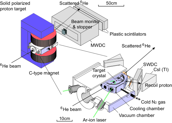
Figure 1: (Color online) Experimental setup of the secondary target and detectors is shown.

A detector system consisted of two subsystems: one for scattered particles and the other for recoil protons. Detection of the recoil protons with energies as low as 10 MeV is essential for the selection of the elastic-scattering events. The scattering angles of protons were determined by single-wire drift chambers (SWDC). The SWDCs were placed 138.5 mm away from the target on both left and right sides of the beam axis as shown in Fig. 1. They covered an angular region of 39^∘–71^∘ (horizontal) and $\pm 9.7^{\circ}$ (vertical) in the laboratory system. Their position resolution and detection efficiency were found to be 2.6 mm (FWHM) and 99.3%. For the measurement of the total energy of protons, we used CsI(Tl) scintillation detectors. They were placed just behind the SWDCs. Light output from the CsI(Tl) crystal was detected by photo-multiplier tubes. The front side of the CsI(Tl) scintillator was covered by the thin carbon-aramid film with a thickness of 12 $\mu$m. Material thickness of the film, the SWDC, and air between the detectors was 24 mg/cm² in total. Energy loss of 10 MeV protons in these materials is 1.2 MeV, which does not prevent the detection.

A multi-wire drift chamber (MWDC) was used to reconstruct the trajectories of scattered particles. Scattering position on the secondary target was determined from the reconstructed trajectory. The MWDC was placed at 880 mm downstream of the target. It has a sensitive area of 640 mm (horizontal) $\times$ 160 mm (vertical) and covered an angular region of $\pm$16${}^{\circ}\times\pm$4^∘ in the laboratory system. The configuration of the planes of the MWDC is X-Y-X’-Y’-X’-Y’-X-Y, where “X(Y)-plane” has anode-wires oriented along the vertical (horizontal) axis. The planes with primes are displaced with respect to the “unprimed” planes by half the cell size. The cell size is 20 mm$\times$20 mm for the X-plane and 10 mm$\times$10 mm for the Y-plane. The material of the anode wire is gold-plated tungsten with a diameter of 30 $\mu$m. Negative high voltages were applied to the cathode and potential wires: $-$2.85 kV for the X (X’)-planes and $-$2.15 kV for the Y (Y’)-planes. A gas mixture of Ar (50%) and C₂H₆ (50%) was used. Position resolution and detection efficiency of the MWDC were found to be 0.2 mm (FWHM) and 99.8%. For identification of scattered particles, we used a plastic scintillation detector array placed just behind the MWDC. The first and second layers with thicknesses of 5 mm and 100 mm provided information of the energy loss and the total energy of scattered particles. The total number of the beam particles was counted with a beam monitor placed between the secondary target and the MWDC. A 50 mm${}^{H}\times$50 mm${}^{V}\times$10 mm^D plastic scintillator was used for the beam monitor. A beam stopper made of a copper block was placed just behind the beam monitor.

II.2 Solid polarized proton target

The solid polarized proton target, used in the measurement, can be operated in a low magnetic field of 0.1 T and at a high temperature of 100 K. These relaxed operation conditions allow us to detect low-energy recoil protons without losing angular resolution. This capability is indispensable to apply the target to scattering experiments carried out under the inverse kinematics condition. The proton polarization of about 20% has been achieved WakuiPST under such relaxed conditions by introducing a new polarizing method using electron polarization in triplet states of photo-excited aromatic molecules Sloop81 ; Henstra88 . A single crystal of naphthalene (C₁₀H₈) doped with a small amount of pentacene (C₂₂H₁₄) is used as the target material. Protons in the crystal are polarized by repeating a two-step process: production of electron polarization and polarization transfer. In the first step, pentacene molecules are optically excited to higher singlet states. A small fraction of them decays to the first triplet state via the first excited singlet state by the so-called intersystem crossing. Here, electron population difference is spontaneously produced among Zeeman sublevels of the triplet state Sloop81 . In the second step, the electron population difference between two Zeeman sublevels, namely electron polarization, is transferred to the proton polarization by the cross-relaxation technique Henstra88 .

As the target material, we used a single crystal of naphthalene doped with 0.005 mol% pentacene molecules. The crystal was shaped into a thin disk whose diameter and thickness are 14 mm and 1 mm (116 mg/cm²), respectively. The number of hydrogens per unit area was 4.29$\pm$0.13$\times 10^{21}$/cm². In order to reduce the relaxation rate, the target crystal was cooled down to 100 K in a cooling chamber with the flow of cold nitrogen gas. The cooling chamber was installed in another chamber as shown in Fig. 1. Heat influx to the cooling chamber was reduced by the vacuum kept in the intervening space between these two chambers. Each chamber has one window (6 $\mu$m-thick Havar foil) on the upstream side for the incoming RI-beam, two glass windows for the laser irradiation, and three windows (20 $\mu$m-thick Kapton foil) on the left, right, and downstream sides for the detection of recoil and scattered particles.

A static magnetic field was applied on the target crystal by a C-type electromagnet to define the polarizing axis. The gap and the diameter of the poles were 100 mm and 220 mm, respectively. The strength of the magnetic field in the present experiment was 91 mT; a value much higher than that of the crystal field ($\approx$ 2 mT). While the effects of the magnetic field on the scattering angles of ⁶He particles and protons were sufficiently small (about 0.07^∘ and 0.2–0.8^∘, respectively), they were properly corrected in the data analysis.

The target crystal was irradiated by the light of two Ar-ion lasers with a power of 25 W each in the multi-line mode. Wavelengths of main components of the light were 514.5 nm (10 W) and 488.5 nm (8 W). The laser light was pulsed by a rotating optical chopper. Typically the pulse width and repetition rate were 12–14 $\mu$s and 1 kHz. Microwave (MW) irradiation and a magnetic field sweep are required in the cross-relaxation method. For the MW irradiation, the target crystal was installed in a resonator. In order to detect low-energy recoil protons, we employed a thin cylindrical loop-gap resonator (LGR Ghim96 ) made of 25 $\mu$m-thick Teflon film. Copper stripes with a thickness of 4.4 $\mu$m were printed on both sides of the film. The MW frequency was 3.40 GHz. The LGR was surrounded by a cylindrical MW shield made of 12 $\mu$m-thick aluminum foil. For the cross-relaxation, the magnetic field was swept from 88 mT to 94 mT at the rate of 0.36 mT/$\mu$s, simultaneously with the MW irradiation, by applying a current to a small coil placed in the vicinity of the target material.

Proton polarization was monitored during the experiment by the pulse NMR method. A radio-frequency (RF) pulse with a frequency and a duration of 3.99 MHz and 2.2 $\mu$s was applied to a 19 mm$\phi$ NMR coil covering the target crystal. The free induction decay (FID) signal was detected by the same coil. We carried out the absolute calibration to relate the FID signal to the proton polarization by measuring the spin-asymmetry in the $p+^{4}$He elastic scattering. Details of the calibration procedure are described in Appendix. A.

Devices located near to the target, namely the LGR, the MW shield, the field sweeping coil, and the NMR coil, were fabricated with hydrogen-free materials to prevent production of background events. Table 1 shows the material thicknesses of the devices that recoil protons penetrate. Energy losses of the 20 MeV protons in these materials are sufficiently small for the detection as summarized in Table 1.

Material	Thickness (mg/cm2)	Energy loss (MeV)
Target crystal (Naphthalene)	0 – 336	0 – 9.5
LGR (Teflon, Cu foil)	9.3	0.2 – 0.4
Microwave shield (Al foil)	3.2	0.05 – 0.1
Cooling gas (N2)	13.5	0.3 – 0.6
Window (Kapton film)	20	0.5 – 1.0
Total	46 – 382	1.1 – 11.6

Table 1: Thicknesses of the materials of target devices and energy losses of 20 MeV recoil protons in them.

The target polarization during the experiment is shown in Fig. 2 as a function of time. The polarization was built up for the first 40 hours and reached the maximum value of 20.4$\pm$3.9%. The target was then irradiated by a 71 MeV/nucleon ⁶He beam for 55 hours, by a 80 MeV/nucleon ⁴He beam for the following 25 hours, and again by the ⁶He beam for 60 hours. The magnitude of average polarization was found to be 13.8$\pm$2.7%. The target polarization slowly decreased as a function of time, which is due to beam-irradiation damage in the target material. This radiation damage increased the relaxation rate of the target material from $\Gamma=$ 0.127(6) h^-1 before the experiment to $\Gamma=$ 0.295(4) h^-1 after the beam irradiation. The direction of the target polarization was reversed three times during the measurement to cancel spurious asymmetries. The 180^∘ pulse NMR method was used here. Reversal efficiency of 60–70% was achieved.

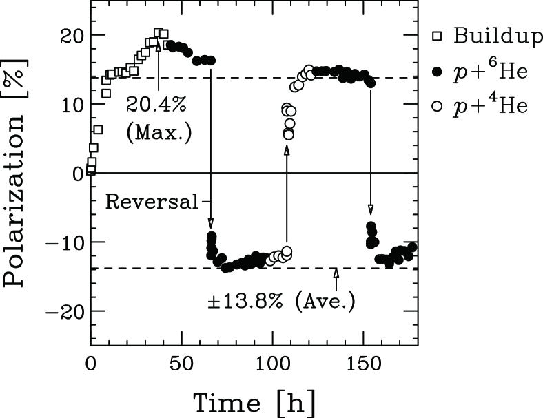
Figure 2: Target polarization is shown as a function of time. The open squares, closed circles, and open circles indicate the target polarization during the polarization buildup, the $p+^{6}$He elastic-scattering measurement, and the $p+^{4}$He elastic-scattering measurement, respectively.

III Data Reduction

III.1 Data analysis

In principle, elastic-scattering events of the ⁶He from protons can be identified by the coincidence detection of scattered ⁶He particles and recoil protons, since the ⁶He does not have a bound excited state. Note that the first excited state of ⁶He, which is the $2^{+}$ state at 1.87 MeV, is above the two-neutron breakup threshold (0.975 MeV). Thus, any excited ⁶He particles decay into $\alpha$+$n$+$n$ systems before reaching the detectors.

Scattered particles were identified by the standard $\Delta E$-$E$ method. Figure 3 shows a two-dimensional plot of the total energies of scattered particles $E$ versus their energy losses $\Delta E$, where loci of tritons, ⁴He, ⁶He, and ⁸Li are found. Tritons and ⁸Li are the contamination in the secondary beam. Most of ⁴He particles were produced by ⁶He dissociation in the secondary target. However, some originated from ⁶He reactions in the plastic scintillators. So to count all of the $p+^{6}$He elastic-scattering events, the particle identification gate includes most of the ⁴He locus as shown by solid curves in Fig. 3. The contribution of the dissociation reaction, which is not excluded by this gate, was subtracted using a kinematics relation. This is described after the response of the recoil proton detectors is considered.

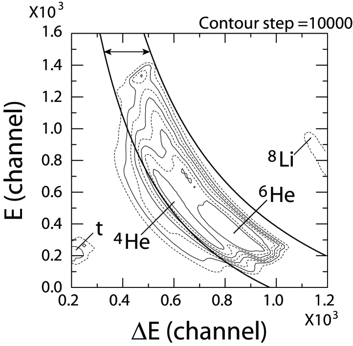
Figure 3: Two-dimensional plot of the total energies of scattered particles versus their energy losses. Solid curves indicate the particle-identification gate.

Figure 4 shows a two-dimensional scatter plot of the proton energies versus their scattering angles in the center-of-mass system, $\theta_{\textrm{c.m.}}$. The kinematic locus of the elastic scattering is clearly identified, while backgrounds from other reaction channels such as $p$(⁶He, $p^{4}$He) are also evident. The kinematic locus of elastic-scattering events shows that the recoil protons were properly detected outside of the target. It should be noted that this correlation was not used for the event selection, since it would cause a loss of the events at forward angles.

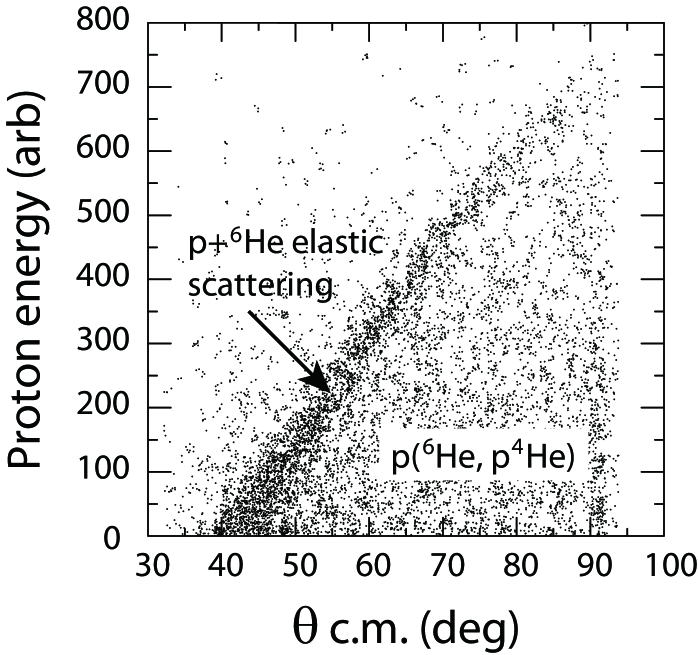
Figure 4: Two-dimensional plot of the proton energies versus their scattering angles.

To discriminate elastic scattering from the background, we used the correlation of the azimuthal angles of protons $\phi_{p}$ with those of scattered particles $\phi_{\textrm{scatt.}}$. In the case of the elastic scattering, a scattered ⁶He and a recoil proton stay within a well defined reaction plane since the final state is a binary system. Thus, the difference of azimuthal angles $\Delta\phi=\phi_{p}-\phi_{\textrm{scatt.}}$ makes a narrow peak at around 180^∘. This back-to-back correlation holds even if the scattered ⁶He is dissociated in the plastic scintillator. In the case of other reactions, however, the azimuthal angle difference is more spread since their final states consist of more than two particles.

Figure 5 shows the distribution of the azimuthal angle difference $\Delta\phi$ fitted by a double-Gaussian function. The narrower component is reasonably identified as that of the elastic-scattering events. The peak width of 3.5^∘ in sigma is consistent with the detector resolution of 3.1^∘. We selected the events of $|\Delta\phi-180^{\circ}|<12.4^{\circ}$. The background remaining in the gate was evaluated from the broader component and was subtracted. Contributions of the inelastic scattering and other reactions such as breakup were removed in this way without losing the elastic-scattering yields. Figure 6 shows a background-subtracted two-dimensional plot of scattering angles in the center-of-mass system versus angles of scattered particles. Center-of-mass scattering angles were deduced from recoil angles of the protons in the laboratory system, since the resolution of scattering angles of ⁶He particles is insufficient due to the kinematic focusing. In Fig. 6, clear peaks of elastic-scattering events lie along the solid curves indicating the kinematics of the $p+^{6}$He elastic scattering. Small peaks at $|\theta_{{}^{6}\textrm{He}}|\approx 4^{\circ}$ originated from the ambiguity in the background subtraction. Yields of the $p+^{6}$He elastic scattering were obtained by counting the events of the elastic-scattering peaks in the typical width of $4^{\circ}$ in $\theta_{{}^{6}\textrm{He}}$.

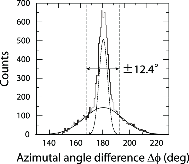
Figure 5: Azimuthal angle difference between scattered particles and recoil protons, fitted by a double-Gaussian function.

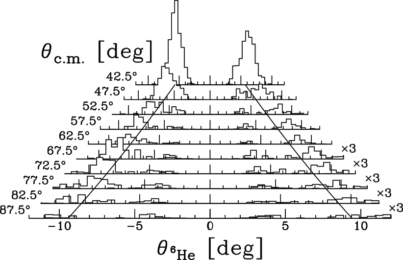
Figure 6: Scattering angle correlation between scattered particles and recoil protons. The solid curves indicate the kinematics of the $p+^{6}$He elastic scattering.

The present work demonstrates the applicability of the solid polarized proton target in the RI-beam experiment. The relaxed operation condition of the target, i.e. a low magnetic field of 0.1 T and high magnetic field of 100 K, enables us to detect the low-energy recoil protons. As described in the data analysis above, information on the trajectory of recoil proton is indispensable both in identifying the elastic-scattering events (Fig. 5) and in deducing the scattering angle (Fig. 6).

III.2 Experimental data

The $d\sigma/d\Omega$ of the $p+^{6}$He elastic scattering measured at 71 MeV/nucleon are summarized in Table 2. In the backward region, the uncertainty mainly results from statistics and from the ambiguity in the background subtraction. In the forward angular region, $\theta_{\textrm{c.m.}}<60^{\circ}$, the main component of the uncertainty in $d\sigma/d\Omega$ is the systematic uncertainty in the number of the incident particles (10%). The target was hit by only a fraction of beam particles since the size of the secondary beam was comparable to that of the target. The percentage of the beam particles incident on the target was determined from the beam profile and was found to be 65$\pm$7% of those counted by the beam monitor. The beam profile was measured with the MWDC by removing the beam stopper. Stability of the beam profile was confirmed by several measurements carried out before, during, and after the elastic-scattering measurement.

The analyzing power $A_{y}$ is deduced with the standard procedure as

$$A_{y}=\frac{1}{P}\frac{L-R}{L+R},\ \ L=\sqrt{N_{L}^{\uparrow}\cdot N_{R}^{\downarrow}},\ \ R=\sqrt{N_{L}^{\downarrow}\cdot N_{R}^{\uparrow}},$$

where $P$ denotes the target polarization. The values $N$’s represent the yield of the elastic-scattering events where subscripts and superscripts denote the scattering direction (left/right) and the polarization direction (up/down), respectively. The statistical uncertainty is expressed by

$$\frac{\Delta A_{y}}{A_{y}}=\frac{LR}{L^{2}-R^{2}}\ \sqrt{\frac{1}{N_{R}^{\uparrow}}+\frac{1}{N_{R}^{\downarrow}}+\frac{1}{N_{L}^{\uparrow}}+\frac{1}{N_{L}^{\downarrow}}}.$$

This procedure allows us to minimize the systematic uncertainties originating from unbalanced detection efficiencies and misalignment of detectors. The obtained $A_{y}$ are summarized in Table 3. It must be noted that there is an additional scale error of 19% resulting from the uncertainty in the target polarization $P$ (see Appendix. A).

$\theta_{\textrm{c.m.}}$ (deg)	$\Delta\theta_{\textrm{c.m.}}$ (deg)	$\frac{d\sigma}{d\Omega}$ (mb/sr)	$\Delta\frac{d\sigma}{d\Omega}$ (mb/sr)
42.1	2.5	5.020	0.520
47.1	2.5	2.030	0.220
52.1	2.5	0.796	0.098
57.4	2.5	0.454	0.059
62.3	2.5	0.360	0.046
67.3	2.5	0.226	0.031
72.3	2.5	0.172	0.023
77.3	2.5	0.127	0.018
82.2	2.5	0.064	0.013
87.2	2.5	0.038	0.012

Table 2: Differential cross sections for the $p+^{6}$He elastic scattering at 71 MeV/nucleon. The $\Delta\theta_{\textrm{c.m.}}$ denotes the bin width. The $\Delta\frac{d\sigma}{d\Omega}$ denotes the quadratic sum of the statistical and systematic uncertainties.

$\theta_{\textrm{c.m.}}$ (deg)	$\Delta\theta_{\textrm{c.m.}}$ (deg)	$A_{y}$	$\Delta A_{y}$
37.1	2.5	$-$0.242	0.069
44.6	5.0	$-$0.021	0.089
54.6	5.0	$-$0.016	0.135
64.8	5.0	$-$0.11$0$	0.18$0$
74.3	5.0	$-$0.27$0$	0.27$0$

Table 3: Analyzing powers for the $p+^{6}$He elastic scattering at 71 MeV/nucleon. $\Delta A_{y}$ denotes the statistical uncertainty. Note that there is an additional scale error of 19% resulting from the uncertainty in the target polarization. The $\Delta\theta_{\textrm{c.m.}}$ denotes the bin width.

Figure 7 shows $d\sigma/d\Omega$ and $A_{y}$ for the $p+^{6}$He elastic scattering at 71 MeV/nucleon (closed circles: present work, open circles: Ref. Korsheninnikov97 ), those for the $p+^{4}$He at 72 MeV/nucleon (open squares: Ref. Burzynski89 ), and those for the $p+^{6}$Li at 72 MeV/nucleon (open triangles: Ref. Henneck94 ). The present data are consistent with the previous ones in Ref. Korsheninnikov97 in an overlapping angular region of $\theta_{\textrm{c.m.}}=40$–$50^{\circ}$. We extended the data to the backward angles of $\theta_{\textrm{c.m.}}\approx 90^{\circ}$. It is found that the $d\sigma/d\Omega$ of $p+^{6}$He are almost identical with those of $p+^{6}$Li at $\theta_{\textrm{c.m.}}=20$–$90^{\circ}$, while they have a steeper angular dependence than those of $p+^{4}$He. In good contrast to the similarity found in $d\sigma/d\Omega$, $A_{y}$ data are widely different between $p+^{6}$He and $p+^{6}$Li. The $A_{y}$ of $p+^{6}$Li increase as a function of the scattering angle in an angular region of $\theta_{\textrm{c.m.}}=40$–$70^{\circ}$ and take large positive values. This behavior is commonly seen in proton elastic scattering from stable nuclei at the present energy region Sakaguchi82 . Unlike this global trend, $A_{y}$ of $p+^{6}$He decreases in $\theta_{\textrm{c.m.}}=37$–$55^{\circ}$, which is rather similar to those of $p+^{4}$He. While the large error bars prevent us from observing the difference between $A_{y}$ of $p+^{6}$He and of $p+^{4}$He, it is clearly seen that the angular distribution of the $A_{y}$ in $p+^{6}$He deviates from that of $p+^{6}$Li.

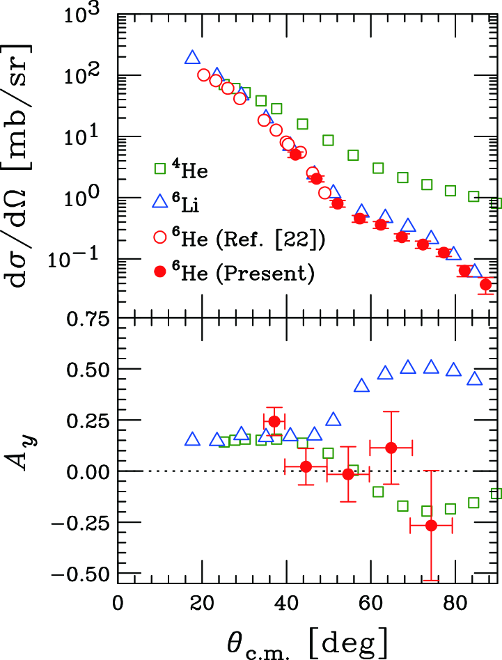
Figure 7: (Color online) Differential cross sections and analyzing powers of the $p+^{4}$He at 72 MeV (open squares: Ref. Burzynski89 ), of the $p+^{6}$Li at 72 MeV (open triangles: Ref. Henneck94 ), and of the $p+^{6}$He at 71 MeV (open circles: Ref. Korsheninnikov97 , closed circles: present work).

IV Phenomenological Optical Model Analysis

IV.1 Optical potential fitting

The aim of this section is to extract the gross characteristics of the spin-orbit interaction between a proton and ⁶He. For this purpose, we determined the optical model potential that reproduces the experimental data of both differential cross sections and analyzing powers. The optical model potential obtained in this phenomenological approach will be compared with the semi-microscopic calculations in Section V.

We adopted a standard Woods-Saxon optical potential with a spin-orbit term of the Thomas form:

$$U_{\textrm{OM}}(R)= - V_{0}\,f_{r}(R)-i\,W_{0}\,f_{i}(R)$$ (1)

$$+ 4i\,a_{id}\,W_{d}\,\frac{d}{dR}f_{id}(R)$$

$$+ V_{s}\,\frac{2}{R}\,\frac{d}{dR}f_{s}(R)\;\bm{L}\cdot\bm{\sigma}_{p}+V_{\textrm{C}}(R)$$

with

$$f_{x}(R) = \left[1+\exp\left(\frac{R-r_{0x}A^{1/3}}{a_{x}}\right)\right]^{-1}\;$$ (2)

$$(x = r,i,id,\ \textrm{or}\ s).$$

Here, $\bm{R}$ is the relative coordinate between a proton and a ⁶He particle (see Fig. 12 (b)), $\bm{L}=\bm{R}\times(-i\hbar\bm{\nabla}_{R})$ is the associated angular momentum, and $\bm{\sigma}_{p}$ is the Pauli spin operator of the proton. The subscripts $r$, $i$, $id$, and $s$ denote real, volume imaginary, surface imaginary, and spin-orbit, respectively. $V_{\textrm{C}}$ is the Coulomb potential of uniformly charged sphere with a radius of $r_{0\textrm{C}}A^{1/3}$ fm ($r_{0\textrm{C}}=1.3$ fm).

The search procedure for the best-fit potential parameters was made in two steps: first the parameters of the central term were found by minimizing the $\chi^{2}$ values of $d\sigma/d\Omega$, and second the parameters of the spin-orbit term by fitting $A_{y}$. These two steps were iterated alternately until convergence was achieved. Such a procedure is feasible since the contribution of the spin-orbit potential to $d\sigma/d\Omega$ is much smaller than those of the central terms. In the fitting, we used the data in Ref. Korsheninnikov97 and the present ones. Uncertainties of $d\sigma/d\Omega$ smaller than 10% were artificially set to 10% in order to avoid trapping in an unphysical local $\chi^{2}$ minimum. The fitting was carried out using the ECIS79 code Raynal65 . A set of parameters for the $p+^{6}$Li elastic scattering at 72 MeV/nucleon Henneck94 , labeled as Set-A in Table 4, was used as the initial values in the search of the $p$-⁶He potential parameters.

Table 4: Parameters of the optical potentials for $p+^{6}$Li at 72 MeV/nucleon Henneck94 and $p+^{6}$He at 71 MeV/nucleon (Gupta00 and present work).

		$V_{0}$	$r_{0r}$	$a_{r}$	$W_{0}$	$r_{0i}$	$a_{i}$	$W_{d}$	$r_{0id}$	$a_{id}$	$V_{s}$	$r_{0s}$	$a_{s}$
		(MeV)	(fm)	(fm)	(MeV)	(fm)	(fm)	(MeV)	(fm)	(fm)	(MeV)	(fm)	(fm)
Set-A	$p+^{6}$Li Henneck94	31.67	1.10	0.75	14.14	1.15	0.56	—	—	—	3.36	0.90	0.94
Set-B	$p+^{6}$He (Present)	27.86	1.074	0.681	16.58	0.86	0.735	—	—	—	2.02	1.29	0.76
Set-C	$p+^{6}$He Gupta00	30.00	0.990	0.612	14.0	1.10	0.690	1.00	1.76	0.772	5.90	0.677	0.630

The parameters obtained for the $p+{}^{6}$He elastic scattering are labeled as Set-B in Table 4. The reduced $\chi^{2}$ values for $d\sigma/d\Omega$ and $A_{y}$ were 0.95 and 0.96, respectively. Uncertainties of the parameters of the spin-orbit potential, $r_{0s}$, $a_{s}$, and $V_{s}$, are evaluated in the following manner. Figure 8 shows the contour map of the deviation of $\chi^{2}$ value for $A_{y}$ from that calculated by the Set-B (as indicated by the point-P), $\Delta\chi^{2}_{A_{y}}$, on the two-dimensional plane of $r_{0s}$ and $a_{s}$ after projecting with optimized $V_{s}$ at each point of the plane. In the figure, a simultaneous confidence region for $r_{0s}$ and $a_{s}$ is presented by the solid contour indicating $\Delta\chi^{2}_{A_{y}}=1$. In this region, the optimum $V_{s}$ ranges between 1.15 MeV (at the point-Q) and 2.82 MeV (at the point-R). In the $r_{0s}$-$a_{s}$-$V_{s}$ space, a surface that $\Delta\chi^{2}_{A_{y}}=1$ touches planes that are expressed by $r_{0s}=1.29\pm 0.13$ fm, $a_{s}=0.76\pm 0.17$ fm, and $V_{s}=2.02\pm 0.87$ MeV, which gives a rough estimation for uncertainties of the parameters.

Figure 8: Contour map of the $\Delta\chi^{2}_{A_{y}}$ values (see the text for the definition) on the two-dimensional plane of $r_{0s}$ and $a_{s}$. The solid, dashed, and dotted curves indicate $\Delta\chi^{2}_{A_{y}}$=1, 3, and 5, respectively. The point that gives the best-fit parameters, Set-B in Table IV, is indicated by the point-P. See the text for the points-Q and -R.

IV.2 Characteristics of spin-orbit potential

In Fig. 9, the results of calculations of the observables made with the optical potentials of Set-A, -B, and -C in Table 4 are shown together with the experimental data. Set-C was taken from Ref. Gupta00 , where a phenomenological optical model potential that reproduced only the previous $d\sigma/d\Omega$ data of the $p+^{6}$He at 71 MeV/nucleon Korsheninnikov97 was reported. The radial dependences of the $p$-⁶He optical potentials (Set-B and Set-C) are shown in Fig. 10 by solid and dashed lines, respectively.

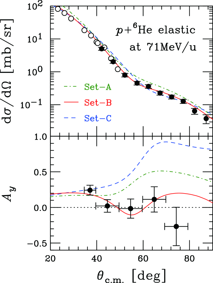
Figure 9: (Color online) Differential cross sections and analyzing powers calculated by the phenomenological optical potentials are shown together with the experimental data. The dot-dashed curves denote calculations of the Set-A in Table 4, the solid curves those of set-B, and the dashed curves those of Set-C. Solid circles are present data and open circles are from Ref. Korsheninnikov97 .

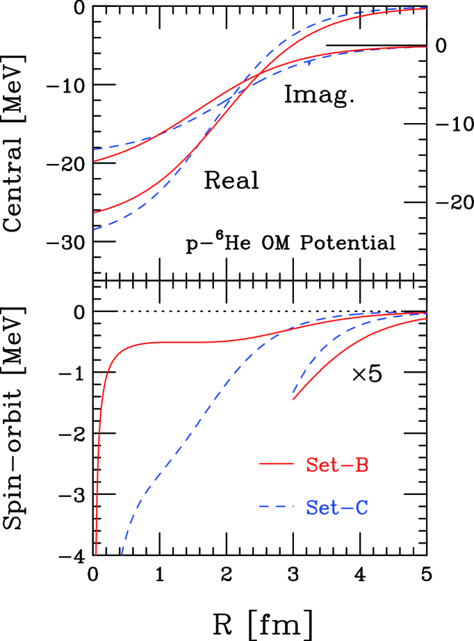
Figure 10: (Color online) Radial dependences of the phenomenological optical potential (Set-B and Set-C in Table 4). Solid and dashed curves in the upper panel represent the real and imaginary parts of the central term. The lower panel shows the spin-orbit potential.

The calculation with the potential Set-C reasonably reproduces the present $d\sigma/d\Omega$ data, whereas it largely deviates from the $A_{y}$ data at $\theta_{\textrm{c.m.}}\gtrsim 40^{\circ}$. It should be noted that the $A_{y}$ data were unavailable when the potential Set-C was sought. The calculation with the potential Set-B reproduces both $d\sigma/d\Omega$ and $A_{y}$ over whole angular region except for the most backward data point of $A_{y}$. Similarity of the $d\sigma/d\Omega$ calculated with Set-B and Set-C potentials originates from that of the central terms as shown in the upper panel of Fig. 10. The reliability of the potential obtained in the present work is supported by the fact that two independent analyses yielded the similar results for the central terms. In contrast to the central terms, the spin-orbit terms of these two potentials are quite different, resulting in a large difference in $A_{y}$ as shown in Fig. 9. Note that the present data are sensitive to the optical potential in a region of $R\gtrsim$1.5 fm. The spin-orbit potential of Set-B is much shallower than that of Set-C at $R\lesssim$ 2.8 fm, while it is deeper at larger radii. This is due to the small value of $V_{s}$ and large values of $r_{0s}$ and $a_{s}$ of Set-B compared with those of Set-C. The phenomenological optical model analysis suggests that the $A_{y}$ data can be reproduced only with a shallow and long-ranged spin-orbit potential.

The parameters of our spin-orbit potential are compared with those of neighboring even-even stable nuclei and with global potentials in Table 5. Phenomenological optical potentials for the $p+^{16}$O at 65 MeV and $p+^{12}$C at 16–40 MeV are taken from Ref. Sakaguchi82 and Refs. Fricke67 ; Fabrici80 , respectively. In addition to these local potentials, we also examined the parameters of global optical potentials: CH89 Varner91 and Koning-Delaroche (KD) Koning03 , of which applicable ranges are $E=$ 10–65 MeV, $A=$ 40–209 and $E=$ 0.001–200 MeV, $A=$ 24–209, respectively. While they are constructed for nuclei heavier than ⁶He, it is worthwhile comparing them, since the mass-number dependence of the parameters is relatively small. For example, the mass-number dependence appears only in $r_{0s}$ in the case of CH89 Varner91 as:

$$V_{s} = 5.9(1)~{}\textrm{MeV},$$

$$r_{0s} = 1.34(3)-1.2(1)A^{-1/3}~{}\textrm{fm},$$

$$a_{s} = 0.63(2)~{}\textrm{fm}.$$

Table 5 includes the parameters of these potentials for the nuclei within the applicable range. Incident energies of $E=$ 65 MeV and $E=$ 71 MeV were assumed here for CH89 and KD, respectively.

	$V_{s}$ (MeV)	$r_{0s}$ (fm)	$a_{s}$ (fm)
$p+^{6}$He, $E=$ 71 MeV (Set-B)	2.02	1.29	0.76
$p+^{12}$C, $E=$ 40 MeV Fricke67	6.18	1.109	0.517
$p+^{12}$C, $E=$ 16–40 MeV Fabrici80	6.4	1.00	0.575
$p+^{16}$O, $E=$ 65 MeV Sakaguchi82	5.793	1.057	0.5807
CH89, $E=$ 65 MeV, $A=$40–209 Varner91	5.9$\pm$0.1	0.99–1.14	0.63$\pm$0.02
KD, $E=$ 71 MeV, $A=$24–209 Koning03	4.369–4.822	0.961–1.076	0.59

Table 5: Parameters of the spin-orbit term of phenomenological and global optical potentials.

Firstly, we focus on $r_{0s}$ and $a_{s}$ to discuss the radial shape of the spin-orbit potential. Combination of different values of $r_{0s}$ and $a_{s}$ can provide similar results of $A_{y}$ since the observable is sensitive to the surface region of the spin-orbit potential. We thus compare these parameters on the two-dimensional plane of $r_{0s}$ and $a_{s}$ as shown in Fig. 11. Parameters for the stable nuclei are mostly distributed in a region of $r_{0s}=0.8$–$1.1$ fm and $a_{s}=0.5$–$0.6$ fm, whereas that for ⁶He is located in the upper right side of the figure. These large $r_{\textrm{0}s}$ and/or $a_{s}$ values indicate that the spin-orbit potential between a proton and a ⁶He has a long-ranged nature compared with those for stable nuclei. The depth parameter $V_{s}$ was also compared with the global systematics. The $V_{s}$ value of $p$-⁶He potential was found to be 2.02 MeV for the best-fit potential (Set-B) and ranges between 1.15 and 2.82 MeV in the simultaneous confidence region for $r_{0s}$ and $a_{s}$. On the other hand, those of stable nuclei are mostly distributed around 5 MeV as shown in Table 5. Comparing these values, the depth parameter of the spin-orbit potential between a proton and a ⁶He is found to be much smaller than those of stable nuclei.

Figure 11: Two-dimensional distribution of $r_{0s}$ and $a_{s}$ of phenomenological OM potentials for $p+^{6}$He (closed circle), $p+^{12}$C (closed triangle: Ref. Fabrici80 , closed diamond: Fricke67 ), and $p+^{16}$O (closed square: Sakaguchi82 ). The solid contour indicates the simultaneous confidence region for the $r_{0s}$ and $a_{s}$ values for the $p+^{6}$He as displayed in Fig. 8. Parameters of global OM potentials Varner91 ; Koning03 are also shown by solid lines which represent the $A$-dependence of $r_{0s}$.

The phenomenological analysis indicates that the spin-orbit potential between a proton and ⁶He is characterized by large $r_{0s}/a_{s}$ and small $V_{s}$ values yielding shallow and long-ranged radial dependence. Intuitively, these characteristics can be understood from the diffused density distribution of ⁶He. However, its microscopic origin can not be clarified by the phenomenological approach. To examine the microscopic origin of the characteristics of the $p$-⁶He interaction, microscopic and semi-microscopic analyses are required. Section V describes one of such analyses based on a cluster folding model for ⁶He.

V Semi-microscopic Analyses

In this section, we examine two kinds of the folding potential, the cluster folding (CF) and the nucleon folding (NF) ones. They are compared with the phenomenological optical model (OM) potential determined in the preceding section. The results of calculations of observables made by these potentials are compared with the experimental data.

In the CF potential, we adopt the $\alpha nn$ cluster model for ⁶He and fold interactions between the proton and the valence neutrons, $V_{pn}$, with the neutron density in ⁶He and those between the proton and the $\alpha$ core, $V_{p\alpha}$, with the $\alpha$ density in ⁶He. In the NF potential, we decompose the $\alpha$ core into two neutrons and two protons and fold the interactions between the incident proton and the four neutrons, $V_{pn}$, with the neutron density in ⁶He and those between the incident proton and two target protons, $V_{pp}$, with the proton density in ⁶He.

The detailed expressions of such folding potentials are given in the following subsection, where the Coulomb interaction is considered in the $p$-$p$ and $p$-$\alpha$ interactions respectively when compared with the corresponding scattering data but finally it is assumed to act between the proton and the ⁶He target with $r_{0\textrm{C}}=1.400$ fm Gupta00 .

V.1 Folding potentials

Denoting two valence neutrons by $n_{1}$ and $n_{2}$, the CF potential $U_{\text{CF}}$ is given as

$$U_{\textrm{CF}} = \int V_{pn_{1}}\,\rho_{n}^{\textrm{CF}}(r_{1})\,d\bm{r}_{1}+\int V_{pn_{2}}\,\rho_{n}^{\textrm{CF}}(r_{2})\,d\bm{r}_{2}$$ (3)

$$+ \int V_{p\alpha}\,\rho_{\alpha}^{\textrm{CF}}(r_{\alpha})\,d\bm{r}_{\alpha}\;,$$

where $\bm{r}_{1}$, $\bm{r}_{2}$, and $\bm{r}_{\alpha}$ are the position vectors of $n_{1}$, $n_{2}$, and the $\alpha$ core from the center of mass of ⁶He, respectively. The neutron and $\alpha$ densities, $\rho_{n}^{\textrm{CF}}$ and $\rho_{\alpha}^{\textrm{CF}}$, are calculated by the $\alpha nn$ cluster model for ⁶He Hiyama96 ; Hiyama03 , where the condition $\bm{r}_{1}+\bm{r}_{2}+4\bm{r}_{\alpha}=0$ is considered as usual.

In the present work, we specify the potentials in the right hand side of Eq. (3) by the central plus spin-orbit (LS) type:

$$V_{pn_{i}}=V^{0}_{pn}(|\bm{r}_{pn_{i}}|)+V^{\text{LS}}_{pn}(|\bm{r}_{pn_{i}}|)\bm{\ell}_{pn_{i}}\cdot(\bm{\sigma}_{p}+\bm{\sigma}_{n_{i}}),$$

where $i=1,2$ and

$$V_{p\alpha}=V^{0}_{p\alpha}(|\bm{r}_{p\alpha}|)+V^{\text{LS}}_{p\alpha}(|\bm{r}_{p\alpha}|)\bm{\ell}_{p\alpha}\cdot\bm{\sigma}_{p}.$$ (4)

Here, $\bm{r}_{pn_{1}}$, $\bm{r}_{pn_{2}}$, and $\bm{r}_{p\alpha}$ are defined in Fig. 12 (a), and $\bm{\ell}_{pn_{1}}=\bm{r}_{pn_{1}}\times(-i\hbar\bm{\nabla}_{pn_{1}})$, etc.

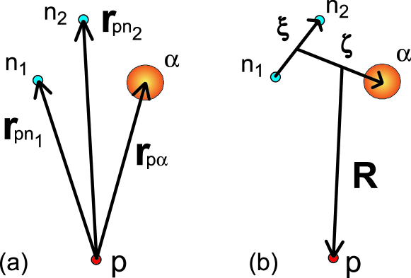
Figure 12: (Color online) Coordinate systems for the cluster folding model.

In the following, we transform the set of coordinates $(\bm{r}_{pn_{1}},\bm{r}_{pn_{2}},\bm{r}_{p\alpha})$ to that of $(\bm{\xi},\bm{\zeta},\bm{R})$, which are defined in Fig. 12 (b), to describe the angular momenta $\bm{\ell}_{pn_{i}}$ and $\bm{\ell}_{p\alpha}$ in terms of $\bm{L}$. The transformation is

$$\bm{r}_{pn_{1}} = -\bm{R}-\frac{2}{3}\bm{\zeta}-\frac{1}{2}\bm{\xi}\;,\;\;\;\bm{r}_{pn_{2}}=-\bm{R}-\frac{2}{3}\bm{\zeta}+\frac{1}{2}\bm{\xi}\;,\;\;\;$$

$$\bm{r}_{p\alpha} = -\bm{R}+\frac{1}{3}\bm{\zeta}\;,$$ (5)

and consequently

$$\bm{\nabla}_{pn_{1}} = -\frac{1}{6}\bm{\nabla}_{R}-\frac{1}{2}\bm{\nabla}_{\zeta}-\bm{\nabla}_{\xi}\;,\;\;\;$$

$$\bm{\nabla}_{pn_{2}} = -\frac{1}{6}\bm{\nabla}_{R}-\frac{1}{2}\bm{\nabla}_{\zeta}+\bm{\nabla}_{\xi}\;,\;\;\;$$

$$\bm{\nabla}_{p\alpha} = -\frac{2}{3}\bm{\nabla}_{R}+\bm{\nabla}_{\zeta}\;.$$ (6)

These relations lead to, for example,

$$\bm{\ell}_{pn_{1}}=(-\bm{R}-\frac{2}{3}\bm{\zeta}-\frac{1}{2}\bm{\xi})\times[-i\hbar(-\frac{1}{6}\bm{\nabla}_{R}-\frac{1}{2}\bm{\nabla}_{\zeta}-\bm{\nabla}_{\xi})]\;.$$ (7)

Here, $\bm{\nabla}_{\xi}$ and $\bm{\nabla}_{\zeta}$ can be neglected, because these are the momenta for the internal degrees of freedom of ⁶He and their expectation values are zero for a spherically symmetric nucleus Rikus84 . Using $\frac{2}{3}\bm{\xi}+\frac{1}{2}\bm{\zeta}=-\bm{r}_{1}$, we get

$$\bm{\ell}_{pn_{1}}=\frac{1}{6}\,[\bm{L}-\bm{r}_{1}\times(-i\hbar\bm{\nabla}_{R})]\;,$$ (8)

which is independent of the special choice of the ⁶He internal coordinates, $\bm{\xi}$ and $\bm{\zeta}$. To $\bm{L}$, $\bm{r}_{1}$ can contribute by its component along the $\bm{R}$ direction Rikus84 , then

$$\bm{\ell}_{pn_{1}}=\frac{1}{6}\,\bm{L}\,(1-\frac{\bm{r}_{1}\cdot\bm{R}}{R^{2}})\;.$$ (9)

Similar expressions are obtained for $\bm{\ell}_{pn_{2}}$ and $\bm{\ell}_{p\alpha}$. Setting $\frac{1}{2}(\bm{\sigma}_{n_{1}}+\bm{\sigma}_{n_{2}})=0$ and considering other quantities to appear in symmetric manners on 1 and 2, we obtain the $p$-⁶He potential as

$$U_{\textrm{CF}}=U_{0}^{\textrm{CF}}(R)+U_{\textrm{LS}}^{\textrm{CF}}(R)\,\bm{L}\cdot\bm{\sigma}_{p}\;,$$ (10)

with

$$U_{0}^{\textrm{CF}}(R) = 2\,\int V_{pn}^{0}(|\bm{r}_{1}-\bm{R}|)\,\rho_{n}^{\textrm{CF}}(r_{1})\,d\bm{r}_{1}$$ (11)

$$+ \int V_{p\alpha}^{0}(|\bm{r}_{\alpha}-\bm{R}|)\,\rho_{\alpha}^{\textrm{CF}}(r_{\alpha})\,d\bm{r}_{\alpha}$$

and

$$U_{\textrm{LS}}^{\textrm{CF}}(R) = \frac{1}{3}\,\int V_{pn}^{\textrm{LS}}(|\bm{r}_{1}-\bm{R}|)\,\left\{1-\frac{\bm{r}_{1}\cdot\bm{R}}{R^{2}}\right\}\,\rho_{n}^{\textrm{CF}}(r_{1})\,d\bm{r}_{1}$$ (12)

$$+ \frac{2}{3}\,\int V_{p\alpha}^{\textrm{LS}}(|\bm{r}_{\alpha}-\bm{R}|)\,\left\{1-\frac{\bm{r}_{\alpha}\cdot\bm{R}}{R^{2}}\right\}\,\rho_{\alpha}^{\textrm{CF}}(r_{\alpha})\,d\bm{r}_{\alpha}\;.$$

In a way similar to the above development, we get the NF model potential $U_{\textrm{NF}}$. In this case, the relative coordinates between the incident proton and six nucleons in the ⁶He nucleus are transformed to the proton-⁶He relative coordinate $\bm{R}$ and a set of five independent internal coordinates of ⁶He. The obtained $U_{\textrm{NF}}$, which is independent on the choice of the set of the internal coordinates, is written as

$$U_{\textrm{NF}}=U_{0}^{\textrm{NF}}(R)+U_{\textrm{LS}}^{\textrm{NF}}(R)\,\bm{L}\cdot\bm{\sigma}_{p}\;,$$ (13)

with

$$U_{0}^{\textrm{NF}}(R) = 2\,\int V_{pp}^{0}(|\bm{r}_{1}-\bm{R}|)\,\rho_{p}^{\textrm{NF}}(r_{1})\,d\bm{r}_{1}$$ (14)

$$+ 4\,\int V_{pn}^{0}(|\bm{r}_{2}-\bm{R}|)\,\rho_{n}^{\textrm{NF}}(r_{2})\,d\bm{r}_{2}$$

and

$$U_{\textrm{LS}}^{\textrm{NF}}(R) = \frac{1}{3}\,\int V_{pp}^{\textrm{LS}}(|\bm{r}_{1}-\bm{R}|)\,\left\{1-\frac{\bm{r}_{1}\cdot\bm{R}}{R^{2}}\right\}\,\rho_{p}^{\textrm{NF}}(r_{1})\,d\bm{r}_{1}$$ (15)

$$+ \frac{2}{3}\,\int V_{pn}^{\textrm{LS}}(|\bm{r}_{2}-\bm{R}|)\,\left\{1-\frac{\bm{r}_{2}\cdot\bm{R}}{R^{2}}\right\}\,\rho_{n}^{\textrm{NF}}(r_{2})\,d\bm{r}_{2}\;,$$

where $\rho_{n}^{\textrm{NF}}$ and $\rho_{p}^{\textrm{NF}}$ denote point neutron and proton densities, respectively.

V.2 Numerical evaluation of $p$-⁶He potentials

To evaluate the $p$-⁶He folding potentials as specified in the preceding section, we have to fix the following elements; the $p$-$\alpha$ interaction $V_{p\alpha}$, the $p$-$p$ and $p$-$n$ interactions $V_{pp}$ and $V_{pn}$, and the densities in ⁶He, $\rho_{\alpha}$, $\rho_{p}$ and $\rho_{n}$. These are discussed in the following subsections, respectively.

V.2.1 $p$-$\alpha$ interactions

For $V_{p\alpha}$ used in the CF potential, we assume the standard WS potential such as given in Eq. (1). The parameters involved are searched so as to fit the data of $d\sigma/d\Omega$ and $A_{y}$ in the $p$+$\alpha$ scattering at 72 MeV/nucleon Burzynski89 . Particular attention was given to reproducing the observables in the forward angular region, since overall agreements with the data are not found in spite of the careful search of the parameters. Two typical parameter sets, with and without the volume absorption term, are labeled as Set-1 and Set-2 in Table  6. The results of calculations made with these potentials are compared with the data in Fig. 13, where the solid and dashed lines show those by Set-1 and Set-2 potentials, respectively. Both calculations describe the data up to $\theta\approx 100^{\circ}$ but do not reproduce those at backward angles, $\theta\gtrsim 120^{\circ}$. Such discrepancies between the calculated results and the measured data at the backward angles suggest participation of contributions of other reaction mechanisms, such as knock-on type exchange scattering of the proton with target nucleons. Such possible extra mechanisms will be disregarded at present since we are concerned with the $p$-$\alpha$ one-body potential. In our CF calculations, we adopt the potentials with the above parameter sets as $V_{p\alpha}$. However, the validity of the CF potential thus obtained is limited to forward scattering angles, a low momentum transfer region, of $p$+⁶He scattering. The real and imaginary parts of $V_{p\alpha}^{0}$ and the real part of $V_{p\alpha}^{\textrm{LS}}$ for the above parameter sets are displayed in the upper and lower panels of Fig. 14. Although Set-1 (dashed) and Set-2 (solid) potentials have rather different $r_{p\alpha}$ dependence, as shown later, this difference is moderated in the folding procedure so yielding similar CF potentials.

Table 6: Parameters for the optical potentials for $p$+⁴He at 72 MeV/nucleon.

	$V_{0}$	$r_{0r}$	$a_{r}$	$W_{0}$	$r_{0i}$	$a_{i}$	$W_{d}$	$r_{0id}$	$a_{id}$	$r_{0\textrm{C}}$	$V_{s}$	$r_{0s}$	$a_{s}$
	(MeV)	(fm)	(fm)	(MeV)	(fm)	(fm)	(MeV)	(fm)	(fm)	(fm)	(MeV)	(fm)	(fm)
Set-1	64.13	0.7440	0.2562	6.338	1.450	0.2089	46.23	1.320	0.1100	1.400	2.752	1.100	0.2252
Set-2	54.87	0.8566	0.09600	—	—	—	31.97	1.125	0.2811	1.400	3.925	0.8563	0.4914

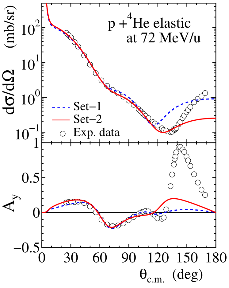
Figure 13: (Color online) Angular distribution of the cross section and $A_{y}$ for the $p+^{4}$He elastic scattering at 72 MeV/nucleon. The solid and dashed lines are the optical model calculations with Set-1 and Set-2 parameters, respectively. The experimental data are taken from Ref. Burzynski89 .

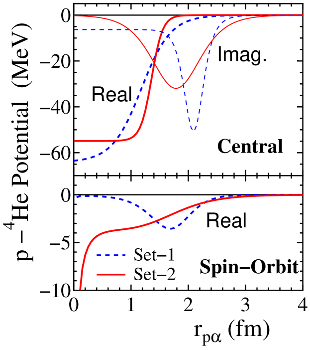
Figure 14: (Color online) Optical potentials for the $p$+⁴He elastic scattering at 72 MeV/nucleon. The thick dashed (solid) lines are for the real part of Set-1 (Set-2) potential and the thin dashed (solid) lines are for the imaginary part.

V.2.2 $p$-$p$ and $p$-$n$ interactions

For $V_{pn}$ and $V_{pp}$ used in the CF and NF potentials, we adopt the complex effective interaction, CEG Yamaguchi83 ; Nagata85 ; Yamaguchi86 , where the nuclear force Tamagaki68 is modified by the medium effect which takes account of the virtual excitation of nucleons of the nuclear matter up to $10k_{\textrm{F}}$ by the $g$-matrix theory. The nuclear force is composed of Gaussian form factors and the parameters contained are adjusted to simulate the matrix elements of the Hamada-Johnston potential Hamada62 . The CEG interaction has been successful in reproducing $d\sigma/d\Omega$ and $A_{y}$ measured for the proton elastic scattering by many nuclei in a wide incident energy range, $E_{p}=$ 20–200 MeV, in the framework of the folding model Yamaguchi83 ; Nagata85 ; Yamaguchi86 . It has been shown that the imaginary part of the folding potential given by the CEG interaction is slightly too large to reproduce experimental N-A scattering Yamaguchi83 ; Yamaguchi86 . In the present calculation, therefore, we adopt the normalizing factor $N_{I}=0.7$ for the imaginary part of the CEG interaction. However, calculations with $N_{I}=1.0$ do not give an essential change to the results.

V.2.3 Densities of $\alpha$, $p$ and $n$ in ⁶He

The densities $\rho_{n}^{\textrm{CF}}$ and $\rho_{\alpha}^{\textrm{CF}}$ for the CF calculation are obtained by applying the Gaussian expansion method Hiyama96 ; Hiyama03 to the $\alpha nn$ cluster model of ⁶He. This method has been successful in describing structures of various few-body systems as well as ⁶He Hiyama96 ; Hiyama03 . As for the $n$-$n$ interaction, we choose AV8’ interaction Wiringa84 . It is reasonable to use a bare (free space) $n$-$n$ interaction between the two valence neutrons in ⁶He as they are dominantly in a region of low density. As for the $\alpha$-$n$ interaction, we employ the effective $\alpha$-$n$ potential in Ref. Kanada79 , which was designed to reproduce well the low-lying states and low-energy-scattering phase shifts of the $\alpha$-$n$ system. The depth of the $\alpha$-$n$ potential is modified slightly to adjust the ground-state binding energy of ⁶He to the empirical value. In Fig. 15(a), the densities obtained are shown as functions of $r$, the distance from the center of mass of ⁶He, where $\rho_{\alpha}^{\textrm{CF}}$ is localized in a relatively narrow region around the center, while $\rho_{n}^{\textrm{CF}}$ is spread widely.

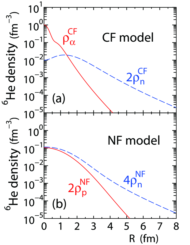
Figure 15: (Color online) The densities of $\alpha$, $p$, and $n$ in ⁶He used in folding models. The $\rho_{\alpha}^{\textrm{CF}}$ and $\rho_{n}^{\textrm{CF}}$ in panel (a) are used in the CF calculation. The $\rho_{p}^{\textrm{NF}}$ and $\rho_{n}^{\textrm{NF}}$ in panel (b) are used in the NF calculation. All densities are normalized as $4\pi\,\int\rho_{\textrm{x}}\,r^{2}\,dr=1$, where $\textrm{x}=\alpha$, $n$, and $p$.

The NF calculation depends on the assumptions made for the densities of the two protons and four neutrons in ⁶He as well as those made for the $p$-$p$ and $p$-$n$ interactions Uesaka10 . At present, to see the essential role of clustering the four nucleons into the $\alpha$-particle core, we use the densities of the proton and the neutron in the $\alpha$ obtained by decomposing the density of the point $\alpha$, $\rho_{\alpha}^{\textrm{CF}}$, to the densities of the constituent nucleons with a one-range Gaussian form factor with range 1.40 fm. The total nucleon densities of ⁶He, $\rho_{p}^{\textrm{NF}}$, and $\rho_{n}^{\textrm{NF}}$, where the latter includes the contribution of the valence neutrons, are displayed in Fig. 15(b). The neutron density $\rho_{n}^{\textrm{NF}}$ has a longer tail than the proton one $\rho_{p}^{\textrm{NF}}$ due to the presence of the valence neutrons. In Refs. ItagakiPrv ; Itagaki03 the nucleon densities of ⁶He were calculated in a more sophisticated way. They produced densities similar to the present ones for the protons and neutrons. These two kinds of nucleon densities provide similar results in the NF calculation of $d\sigma/d\Omega$ and $A_{y}$ of the $p+^{6}$He scattering. Thus, in the following, we will discuss $U_{\textrm{NF}}$ as formed using the densities shown in Fig. 15(b).

V.2.4 $p$-⁶He folding potentials

In Fig. 16, the resultant $p$-⁶He potentials, $U_{\textrm{CF}}$ and $U_{\textrm{NF}}$, are compared with each other as well as with the optical model potential $U_{\textrm{OM}}$. The CF potentials calculated by the two sets of $V_{p\alpha}$ in Table 6, say $U_{\textrm{CF-1}}$ and $U_{\textrm{CF-2}}$, are shown by long-dashed and solid lines in Fig. 16(a), respectively. The folding procedure gives similar results in both cases. The contribution of $V_{pn}$ is displayed by short-dashed lines in the figure, which is found to be mostly small. Especially, in the spin-orbit potential, the contribution from $V_{pn}$ is one order of magnitude smaller than that from $V_{p\alpha}$. The main contribution to $U_{\textrm{CF}}$ arises from the interaction $V_{p\alpha}$ except for the central real potential at $R\gtrsim$3 fm, which is dominated by the $V_{pn}$ contribution. This is supposed to be the reflection of the extended neutron density shown in Fig. 15 and produce significant contributions to the observables as discussed later.

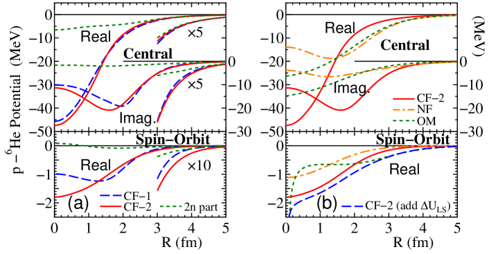
Figure 16: (Color online) Potentials between proton and ⁶He. (a): The long-dashed (solid) lines are the CF calculation with Set-1 (Set-2) parameters for $V_{p\alpha}$. The short-dashed lines show the contribution of the valence two neutrons to the CF potential. (b): The solid lines are the CF calculation with Set-2 parameters, the dot-dashed lines are the NF one and the short-dashed lines are the phenomenological optical potential. The CF spin-orbit potential corrected by $\Delta U_{\textrm{LS}}$ term is shown by the long-dashed line (see text for detail).

In Fig. 16(b), $U_{\textrm{CF}}$ due to Set-2 of $V_{p\alpha}$, $U_{\textrm{NF}}$, and $U_{\textrm{OM}}$ are shown by solid, dot-dashed, and short-dashed lines, respectively. First we consider the central part of the potentials. For small $R$, the real part of $U_{0}^{\textrm{CF}}$ is deeper than those of $U_{0}^{\textrm{NF}}$ and $U_{0}^{\textrm{OM}}$, while for large $R$, $U_{0}^{\textrm{CF}}$ is shallower than other two. In the imaginary part, the magnitude of $U_{0}^{\textrm{CF}}$ is much bigger than those of the other two potentials. This will compensate the deficiency of the real part of $U_{0}^{\textrm{CF}}$ at large $R$, for example in the calculation of the cross section. On the other hand, the spin-orbit part of $U_{\textrm{OM}}$ has larger magnitude for $R\gtrsim 2$ fm and thus has a longer range compared with those of other two potentials. Such long-range nature of the spin-orbit interaction is a characteristic feature of the spin-orbit part of $U_{\textrm{OM}}$ as described in Section IV. This is discussed later in more detail with relation to $A_{y}$.

V.3 Comparison between experiments and calculations in $\bm{p}$+⁶He scattering

In the following, the $d\sigma/d\Omega$ and $A_{y}$ for $p$-⁶He elastic scattering calculated using $U_{\textrm{CF}}$, $U_{\textrm{NF}}$, and $U_{\textrm{OM}}$ are compared with the data taken at 71 MeV/nucleon. In Fig. 17(a) the results obtained using the two CF potentials, $U_{\textrm{CF-1}}$ and $U_{\textrm{CF-2}}$, are shown by long-dashed and solid lines, respectively. Both results are very similar to each other and well describe the data of $d\sigma/d\Omega$, except for large angles where the calculations overestimates the data by small amounts. The calculations also describe the angular dependence of the measured $A_{y}$ up to $\theta\simeq 55^{\circ}$. These successes basically support the CF potential as a reasonable description of the scattering. The discrepancies at large angles, i.e. a large momentum transfer region, may be related to the limitation of the validity of $V_{p\alpha}$ used in the folding, as discussed in the subsection V.2.

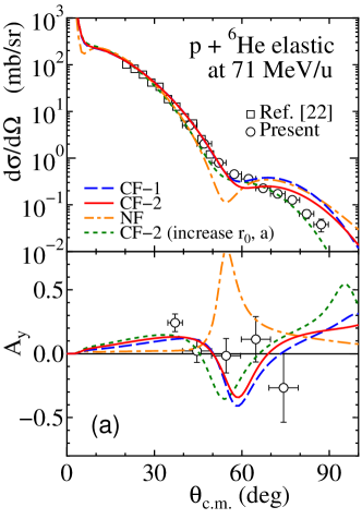
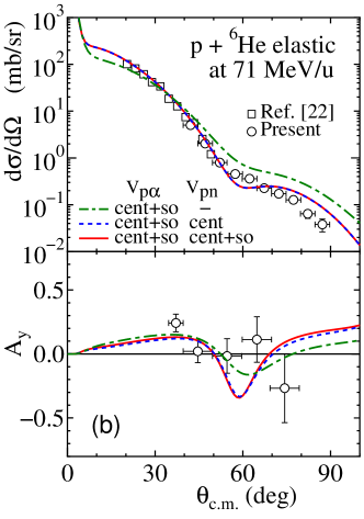
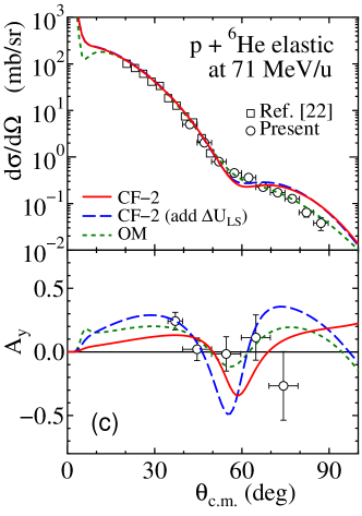
Figure 17: (Color online) Angular distribution of the cross section and $A_{y}$ for the $p$+⁶He elastic scattering at 71 MeV/nucleon. The experimental data are denoted by circles (present) and squares (Ref. Korsheninnikov97 ). (a): The long-dashed (solid) lines are the CF calculation in which Set-1 (Set-2) parameters are used for $V_{p\alpha}$. The dot-dashed lines are the NF calculation. (b): The dashed lines and the solid ones include the $V_{pn}$ interaction, where the formers neglect the spin-orbit part of $V_{pn}$. The dash-dotted lines include only $V_{p\alpha}$ interaction. (c): The solid lines are the CF calculation with Set-2 parameters for $V_{p\alpha}$ and the short-dashed lines are the OM calculation. The long-dashed lines are the CF calculation with Set-2 parameters for $V_{p\alpha}$ where $\Delta U_{\textrm{LS}}$ is added (see text for detail).

In Fig. 17(a), the results of the calculation made using the NF potential are shown by dot-dashed lines. They do not reproduce the data well. The calculation gives an deep valley around $\theta\simeq 53^{\circ}$ in the angular distribution of $d\sigma/d\Omega$ and a large positive peak at the corresponding angle of the $A_{y}$ angular distribution. These features do not exist in the data. Since the present nucleon densities originated from the CF model ones, the essential difference between the CF and NF potentials will be produced by the use of the different interactions. Thus, the CF calculation will owe its successes to the inclusion of the characteristics of the realistic $p$-$\alpha$ interaction into the $p$-⁶He potential.

It is interesting to examine if the $\alpha$ core in ⁶He is somewhat diffused compared with a free $\alpha$-particle, due to the interactions from the valence neutrons. For that purpose, we increased the radius and diffuseness parameters, $r_{0}$ and $a$, in $V_{p\alpha}$ potential as $r_{0}$ to $1.1\,r_{0}$ and $a$ to $a+0.1$ fm. The depth parameters were changed to keep constant the values of the corresponding volume integrals. The effect of this change is shown by the short-dashed lines in Fig. 17(a), where reproduction of the data is improved somewhat, especially in $d\sigma/d\Omega$ at large angles.

In Fig. 17(b), the contributions of the valence neutrons are demonstrated for the CF-2 calculation. As is speculated from the analyses of the form factors of the potential in Fig. 16(a), the dominant contribution to the observables in the CF calculation arises from $V_{p\alpha}$ displayed by the dot-dashed lines in Fig. 17(b). However, the valence neutrons produce indispensable corrections to the observables. That is, the $pn$ central interaction decreases $d\sigma/d\Omega$ at large angles, giving remarkable improvements of the agreement with the data as shown by the dashed lines. The $pn$ interaction also contributes to $A_{y}$ by a considerable amount through the central part. A detailed examination of the calculation revealed that such corrections were due to the $V_{pn}$ part of the folding central potential in a $R$ region between $R=$2 fm and 4 fm (see Fig. 16(a)). The spin-orbit part of $V_{pn}$ gives almost no effect to the observables as shown by the solid lines in Fig. 17(b). This is consistent with the result shown by Crespo et al. Crespo07 in a study at higher incident energy.

In Fig. 17(c), we compared the results of the CF-2 calculation (solid lines) with those of the OM calculation in the preceding section (long-dashed lines) as well as with the data. In the optical model analysis, the experimental data can be reproduced only with a shallow and long-ranged spin-orbit potential. Compared with this potential, the spin-orbit part of CF-2 potential has a shorter range as displayed by a solid line in the lower panel of Fig. 16(b). To investigate the role of the long tail in the spin-orbit potential, we calculated the observables by adding a weak but long-range spin-orbit interaction $\Delta U_{\textrm{LS}}$ to the CF interaction. This correction is assumed to be the Thomas type as

$$\Delta U_{\textrm{LS}}(R)=v_{\textrm{add}}\,\frac{2}{R}\,\frac{d}{dR}\,\left[1+\exp\left\{(R-6^{1/3}r_{\textrm{add}})/a_{\textrm{add}}\right\}\right]^{-1}\;.$$ (16)

For simplicity, we adopt $v_{\textrm{add}}=1$ MeV, $r_{\textrm{add}}=1.5$ fm, and $a_{\textrm{add}}=0.7$ fm where the large magnitudes of $r_{\textrm{add}}$ and $a_{\textrm{add}}$ are consistent with the characteristics of the magnitudes of $r_{0s}$ and $a_{s}$ of the OM potential discussed in Sec. IV. The calculated observables are displayed in Fig. 17(c) by short-dashed lines, where $d\sigma/d\Omega$ is little affected but $A_{y}$ receives a drastic change, i.e. the angular distribution of $A_{y}$ is now similar to that by the OM calculation in a global sense showing qualitative improvements in comparison with the data. To see the contribution of $\Delta U_{\textrm{LS}}$ to the potential, we plot $U_{\textrm{LS}}^{\textrm{CF}}+\Delta U_{\textrm{LS}}$ in Fig. 16(b) by long-dashed lines, where the new spin-orbit potential becomes very close to that of the OM potential at $R\gtrsim 2.5$ fm. It is indicated that the long tail of the spin-orbit potential is particularly important in reproducing the angular distribution of $A_{y}$, while its microscopic origin is still to be investigated. When some corrections which increase the range of the spin-orbit interaction are found, they will be effective for improving the CF calculation.

VI Microscopic Model Analyses

In this section, we will describe the theoretical analysis of the present data by a microscopic model developed in Ref. Amos00 . In this model, one can predict the scattering observables such as cross sections and analyzing powers with one run of the relevant code (DWBA98) with no adjustable parameter. Complete details as well as many examples of use of this coordinate space microscopic model approach are to be found in the review Amos00 . Use of the complex, non-local, nucleon-nucleus optical potentials defined in that way, without localization of the exchange amplitudes, has given predictions of differential cross sections and spin observables that are in good agreement with data from many nuclei (³He to ²³⁸U) and for a wide range of energies (40 to 300 MeV). Crucial to that success is the use of effective nucleon-nucleon ($NN$) interactions built upon $NN$ $g$-matrices. The effective $NN$ interactions are complex, energy and density dependent, admixtures of Yukawa functions. They have central, two-nucleon tensor and two-nucleon spin-orbit character. The $NA$ optical potentials result from folding those effective interactions with the one-body density matrix elements (OBDME) of the ground state in the target nucleus. Antisymmetrization of the projectile with all target nucleons leads to exchange amplitudes, making the microscopic optical potential non-local. For brevity, the optical potentials that result are called $g$-folding potentials. Another application has been in the prediction of integral observables of elastic scattering of both protons and neutrons, with equal success De01 . Thus, the method is known now to give good predictions of both angular-dependent and integral observables.

It is important to note that the level of agreement with data in the $g$-folding approach depends on the quality of the structure model that is used. Due to the character of the hadron force, proton scattering is preferentially sensitive to the neutron matter distributions of nuclei; a sensitivity seen in a recent assessment, using proton elastic scattering, of diverse Skyrme-Hartree-Fock model structures for ²⁰⁸Pb Ka02 .

VI.1 Structure of ⁶He used

⁶He is a two-neutron halo nucleus and has been described well by shell model calculations. In calculation of the $g$-folding potential for protons interacting with ⁶He, a complete $(0$+$2$+$4)\hbar\omega$ shell model calculation has been made to specify the ground state OBDME. Essentially they are the occupation numbers which define the matter densities of the nucleus.

In the present study, we assume three sets of the single-nucleon (SN) wave functions for ⁶He. One is the oscillator wave functions with an oscillator length of 2.0 fm (HO set). However, a neutron-halo character of ⁶He can not be given by the oscillator wave function whatever oscillator length is used as shown by the dashed curve in the lower panel of Fig. 18. Thus, we assume two sets of SN wave functions defined in Woods-Saxon (WS) potentials. One of them is obtained by taking the geometry of the potential from that found appropriate in Ref. Amos00 , where electron form factors and proton scattering from ^6,7Li are studied. That study provided a set of SN wave functions that we specify as WS nonhalo set since the $p$-shell nucleons were all reasonably bound. The extended neutron matter character of ⁶He is found by choosing the binding energy of the halo-neutron orbits to give the single-neutron separation energy (1.8 MeV) to the lowest energy resonance in ⁵He. The set of SN wave functions that result are specified as WS halo set. The associated density profile has the extensive neutron density coming from the halo. Density profiles given by the various sets of SN wave functions are shown in Fig. 18. The dashed, solid, and dot-dashed curves show the density distributions of HO, WS halo, and WS nonhalo sets, respectively. The difference between proton distributions of WS halo and WS nonhalo sets can not be seen.

Figure 18: The (model) proton and neutron densities are shown in the upper and lower panels, respectively. The solid, dot-dashed, and dashed curves represent those obtained with WS halo, WS nonhalo, and HO sets, repectively.

Use of WS halo set in analyses of 40.9 MeV/nucleon data Lagoyannis01 gave a value of 406 mb for the reaction cross section, which is in good agreement with the measured value. Additional evidence for WS halo set is given by the root mean square (r.m.s.) radius of the matter distribution, which is most sensitive to characteristics of the outer surface of a nucleus. Using WS nonhalo set of the SN wave functions gave an r.m.s. radius for ⁶He of 2.30 fm, which is much smaller than the expected value of 2.54 fm. On the other hand, using WS halo set gave an r.m.s. radius for ⁶He of 2.59 fm in good agreement with that expectation.

VI.2 Differential cross sections and analyzing powers

The cross sections and analyzing powers for the $p+^{6}$He elastic scattering at 71 MeV/nucleon are shown in the top and bottom panels of Fig. 19, respectively. The calculated results shown therein by the dashed lines were found using the $g$-folding potential obtained with HO set of SN wave functions. This calculation does not give a satisfactory result; especially in the case of the analyzing power. The solid curves show results found using WS halo set while those depicted by the dot-dashed curves are those found with WS nonhalo set. Of these the halo description gives the better match to data especially at the larger scattering angles. This result is consistent with the findings from analyses of lower energy scattering data at 40.9 MeV/nucleon Lagoyannis01 and at 24.5 MeV/nucleon Stepantsov02 .

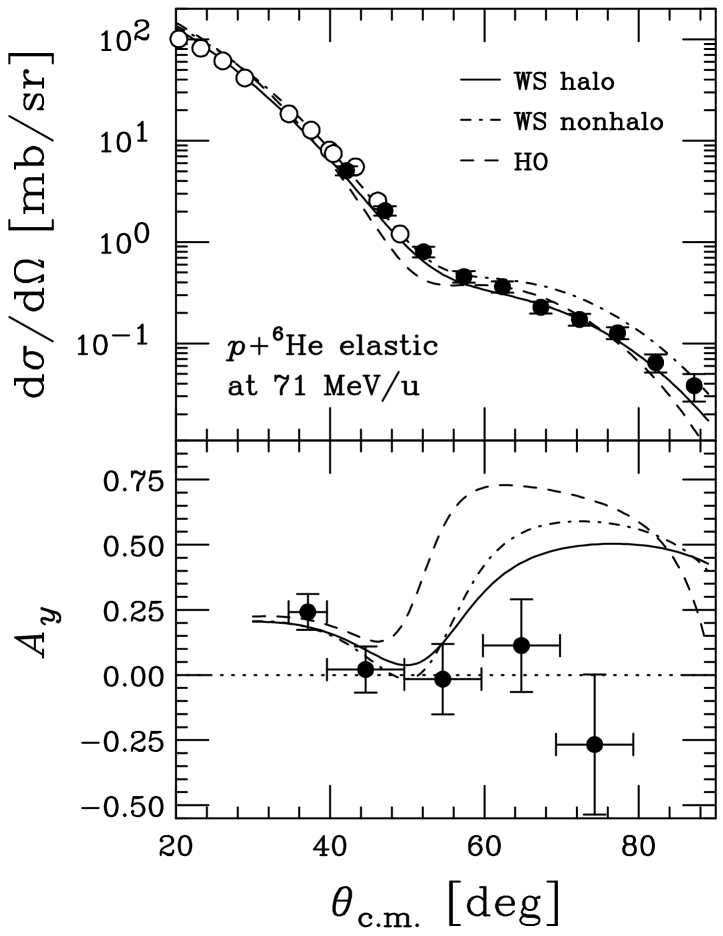
Figure 19: Differential cross sections and analyzing powers of the $p+^{6}$He elastic scattering at 71 MeV/nucleon (open circles: Ref. Korsheninnikov97 , closed circles: present work). Three curves are results of $g$-matrix folding calculation with ⁶He densities presented in Fig. 18.

In fact, the differential cross sections calculated with WS halo set match the data so well that one does not need to contemplate any adjustment. However, the story is not so simple when one also considers the analyzing power data. At forward scattering angles, both WS sets reasonably match the data. But neither WS result produces the distinctive trend of small values found at larger scattering angles. Nonetheless the best result is that found on using WS halo set of SN functions. Given that the cross section values in the region of 60^∘ to 90^∘ is of an order of 0.1 mb/sr, the limitations in the present microscopic model formulation of the reaction dynamics may be the problem.

VII Summary

The vector analyzing power has been measured for the elastic scattering of ⁶He from polarized protons at 71 MeV/nucleon to investigate the characteristics of the spin-orbit potential between the proton and the ⁶He nucleus. Measurement of the polarization observable was realized in the RI-beam experiment by using the newly constructed solid polarized proton target, which can be operated in a low magnetic field of 0.1 T and at high temperature of 100 K. The measured $d\sigma/d\Omega$ of the $p+^{6}$He elastic scattering were almost identical to those of the $p+^{6}$Li. On the other hand, the $A_{y}$ were found to be largely different from those of the $p+^{6}$Li and rather similar to those of the $p+^{4}$He elastic scattering.

To extract the gross feature of the spin-orbit interaction between a proton and ⁶He, an optical model potential was determined phenomenologically by fitting the experimental data of $d\sigma/d\Omega$ and $A_{y}$. Compared with the global systematics of the potentials for stable nuclei, it is indicated that the spin-orbit potential for ⁶He is characterized by a small value of $V_{s}$ and large values of $r_{0s}$ and $a_{s}$, namely by a shallow and long-ranged radial shape. Such characteristics might be the reflection of the diffused density of the neutron-rich ⁶He nucleus.

The cluster folding calculation was carried out to get a deeper insight into the optical potential, assuming the $\alpha$+$n$+$n$ cluster structure for ⁶He. In addition, nucleon folding calculations were also performed by decomposing the $\alpha$ core into four nucleons. The experimental data could not be reproduced by the nucleon folding calculation, whereas the $\alpha nn$ cluster folding calculation gives the reasonable agreements with the data. Thus, this indicates that it is important to take into account of the $\alpha$-clusterization in the description of $p+^{6}$He elastic scattering. The cluster folding calculation shows that the dominant contribution to the $p$-⁶He potential arises from the interaction between the proton and the $\alpha$ core. Especially, in the spin-orbit potential, the contribution of the interaction between the proton and valence neutrons was found to be much smaller than the $\alpha$ core contribution. However, the measured cross section at large angles can not be understood without the contribution from the scattering by the valence neutrons. Comparison of the phenomenological optical potential and the cluster folding one indicates that the long-range nature of the spin-orbit potential is important in reproducing the $A_{y}$ data at large angles. The microscopic origin of such a long tail is still to be investigated.

The data were also compared with the predictions obtained from a fully microscopic $g$-folding model. Three sets of single nucleon wave functions were tried since other details of the calculation were predetermined. The model, which has been successful in analyzing $p$+⁶He scattering cross sections in the past Ka02 , again gives good reproduction of the data in the present case when the bound state wave functions specify that ⁶He has a neutron halo. However, the match to the data, in particular the analyzing power, is not perfect. This may indicate limitation of the structure model used and/or of unaccounted reaction mechanisms that influence the larger momentum transfer results.

This work has demonstrated the capability of the solid polarized proton target in low magnetic field and high temperature to probe the new aspects of the reaction involving unstable nuclei. Future polarization studies of such kinds will provide us with valuable information on the reaction and structure of unstable nuclei.

Appendix A Absolute measurement of target polarization

In the case of conventional solid polarized targets, the NMR signal usually is related to the absolute magnitude of the polarization by measuring the target polarization under the state of thermal equilibrium (TE). However, measurement of the TE polarization is quite difficult in our target. The first reason for this is that the TE polarization is very small in a low magnetic field and at high temperature, since it is represented by $P_{\textrm{TE}}=\tanh\left(\frac{\mu B}{2kT}\right)$, where $\mu,B$, and $T$ are the magnetic moment of proton, the field strength, and the temperature, respectively. The second reason is that the sensitivity of the present NMR system is not sufficiently high since the target design is optimized for scattering experiments.

One of the simple methods to measure the absolute target polarization would be the measurement of the spin-dependent asymmetry $\epsilon=P_{y}A_{y}$ for the proton elastic scattering whose analyzing power $A_{y}$ are known. In the present study, we measured the spin-asymmetry for the $p+^{4}$He elastic scattering at 80 MeV/nucleon. The $A_{y}$ have already been measured by Togawa et al Togawa87 . The use of the $p+^{4}$He scattering is profitable since we can measure the $\epsilon$ with the same experimental setup as that for the $p+^{6}$He measurement only by changing settings of the fragment separator RIPS to produce a secondary ⁴He beam. The profile of the ⁴He beam on the target was tuned to be almost same as that of the ⁶He beam.

Figure 20 shows $A_{y}$ of the $p+^{4}$He elastic scattering at 80 MeV/nucleon. The open circles represent the previous data Togawa87 , while the closed ones show the present data whose magnitudes are scaled to the previous ones. From the scaling factor, the average polarization during the $p+^{4}$He measurement was determined to be $P_{y}=12.3\pm 2.4$%. The relative uncertainty of the polarization $\Delta P_{y}/P_{y}$, which was 19% in the present work, resulted from the statistics of the $p+^{4}$He scattering events. Future development of the NMR system would be required for determining the absolute polarization more precisely without losing beam time.

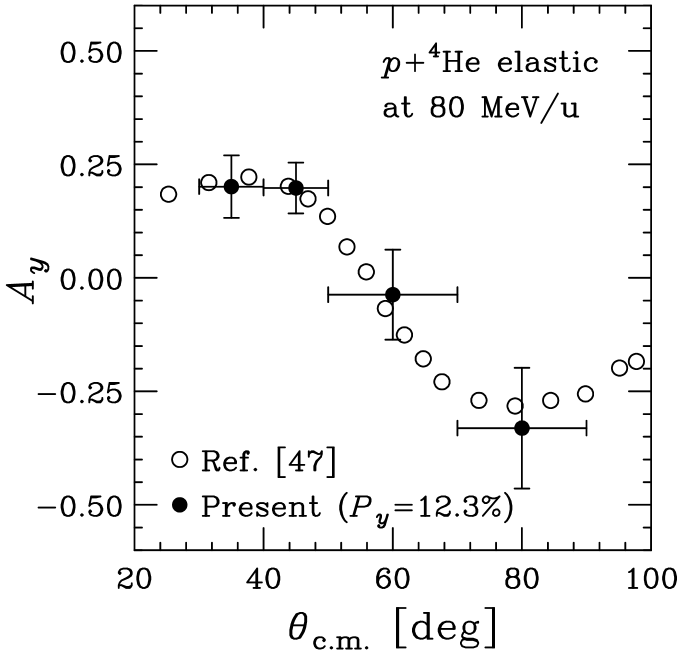
Figure 20: Analyzing powers of the $p+^{4}$He elastic scattering at 80 MeV/nucleon. Closed circles indicate the present data where $P_{y}=12.3\%$ is assumed. Open circles represent the reference data taken from Ref. Togawa87 .

References

- (1) C. L. Oxley et al., Physical Review 91, 419 (1953).
- (2) O. Chamberlain et al., Physical Review 102, 1659 (1956).
- (3) E. Fermi, Nuovo Cimento 10, 407 (1954).
- (4) R. L. Varner et al., Physics Reports (Review Section of Physics Letters) 201, 58 (1991).
- (5) A. Koning and J. Delaroche, Nuclear Physics A 713, 231 (2003).
- (6) F. Brieva and J. Rook, Nucl. Phys. A 297, 1978 (206).
- (7) K. Amos et al., Advances in Nuclear Physics A 25, 275 (2000).
- (8) I. Tanihata et al., Physics Letters B 160, 380 (1985).
- (9) D. Crabb and W. Meyer, Annu. Rev. Nucl. Part. Sci. 47, 1997 (67).
- (10) S. Goertz, W. Meyer, and G. Reicherz, Prog. Part. Nucl. Phys. 49, 403 (2002).
- (11) T. Wakui et al., Nuclear Instruments and Methods in Physics Research A 526, 182 (2004).
- (12) T. Uesaka et al., Nuclear Instruments and Methods in Physics Research A 526, 186 (2004).
- (13) T. Wakui et al., Nuclear Instruments and Methods in Physics Research A 550, 521 (2005).
- (14) M. Hatano et al., European Physical Journal A Supplement 25, 255 (2005); M. Hatano, Ph.D. thesis, University of Tokyo, 2003.
- (15) T. Wakui, Proc. XIth Int. Workshop on Polarized Ion Sources and Polarized Gas Targets 2005, edited by T. Uesaka, H. Sakai, A. Yoshimi, and K. Asahi (World Scientific, Singapore, 2007).
- (16) D. Sloop, T. Yu, T. Lin, and S. Weissman, Journal of Chemical Physics 75, 3746 (1981).
- (17) A. Henstra, P. Dirksen, and W. T. Wenckebach, Physics Letters A 134, 134 (1988).
- (18) T. Uesaka et al., Physical Review C 82, 021602(R) (2010).
- (19) A. Yoshida et al., Nuclear Instruments and Methods in Physics Research A 590, 204 (2008).
- (20) T. Kubo et al., Nuclear Instruments and Methods in Physics Research B 70, 309 (1992).
- (21) B. T. Ghim et al., Journal of Magnetic Resonance A 120, 72 (1996).
- (22) A. Korsheninnikov et al., Nuclear Physics A 617, 45 (1997).
- (23) S. Burzynski et al., Physical Review C 39, 56 (1989).
- (24) R. Henneck et al., Nuclear Physics A 571, 541 (1994).
- (25) H. Sakaguchi et al., Physical Review C 26, 944 (1982).
- (26) J. Raynal, ECIS code, CEA-R2511 Report, unpublished, 1965.
- (27) D. Gupta, C. Samanta, and R. Kanungo, Nuclear Physics A 674, 77 (2000).
- (28) M. Fricke, E. Gross, B. Morton, and A. Zucker, Physical Review 156, 1207 (1967).
- (29) E. Fabrici et al., Physical Review C 21, 830 (1980).
- (30) E. Hiyama et al., Physical Review C 53, 2075 (1996).
- (31) E. Hiyama, Y. Kino, and M. Kamimura, Progress in Particle and Nuclear Physics 51, 223 (2003).
- (32) L. Rikus and H. von Geramb, Nuclear Physics A 426, 496 (1984).
- (33) N. Yamaguchi, S. Nagata, and T. Matsuda, Progress of Theoretical Physics 70, 459 (1983).
- (34) S. Nagata, M. Kamimura, and N. Yamaguchi, Progress of Theoretical Physics 73, 512 (1985).
- (35) N. Yamaguchi, S. Nagata, and J. Michiyama, Progress of Theoretical Physics 76, 1289 (1986).
- (36) R. Tamagaki, Progress of Theoretical Physics 39, 91 (1968).
- (37) T. Hamada and I. Johnston, Nuclear Physics 34, 382 (1962).
- (38) R. Wiringa, R. Smith, and T. Ainsworth, Physical Review C 29, 1207 (1984).
- (39) H. Kanada, T. Kaneko, S. Nagata, and M. Nomoto, Progress of Theoretical Physics 61, 1327 (1979).
- (40) N. Itagaki, private communication.
- (41) N. Itagaki, K. Kobayakawa, and S. Aoyama, Physical Review C 68, 054302 (2003).
- (42) R. Crespo and A. M. Moro, Physical Review C 76, 054607 (2007).
- (43) P. K. Deb et al., Physical Review Letter 86, 3248 (2001).
- (44) S. Karataglidis et al., Physical Review C 65, 044306 (2002).
- (45) A. Lagoyannis et al., Physics Letters B 518, 27 (2001).
- (46) S. V. Stepantsov et al., Physics Letters B 542, 35 (2002).
- (47) H. Togawa and H. Sakaguchi, RCNP Annual Report 1 (1987).