Signal and noise simulation of CUORE bolometric detectors

Abstract

Bolometric detectors are used in particle physics experiments to search for rare processes, such as neutrinoless double beta decay and dark matter interactions. By operating at cryogenic temperatures, they are able to detect particle energies from a few keV up to several MeV, measuring the temperature rise produced by the energy released. This work focusses on the bolometers of the CUORE experiment, which are made of TeO₂ crystals. The response of these detectors is nonlinear with energy and changes with the operating temperature. The noise depends on the working conditions and significantly affects the energy resolution and the detection performances at low energies. We present a software tool to simulate signal and noise of CUORE-like bolometers, including effects generated by operating temperature drifts, nonlinearities and pileups. The simulations agree well with data.

1 Introduction

Bolometers are detectors in which the energy from particle interactions is converted to heat and measured via their rise in temperature. They provide excellent energy resolution, though their response is slow compared to electronic or photonic detectors. These features make them a suitable choice for experiments searching for rare processes, such as neutrinoless double beta decay (0$\nu$DBD) and dark matter (DM) interactions.

The CUORE experiment will search for 0$\nu$DBD of ${}^{130}\mathrm{Te}$ [1, 2] using an array of 988 $\mathrm{TeO}_{2}$ bolometers of 750$\mathrm{\,g}$ each. It may also be sensitive to DM interactions [3]. Operated at a temperature of about 10$\mathrm{\,mK}$, these detectors exhibit an energy resolution of a few keV over an energy range extending from a few keV up to several MeV. In this range the response function is found to be nonlinear [4]. The conversion from signal amplitude to energy is complicated and the shape of the signal depends on the energy itself. Moreover, the amplitude of the signal depends on the temperature of the detector, which is very difficult to keep stable with current cryostats within the few ppm level, the level that would not perturb the energy resolution. The noise of the detector is dominated by thermal fluctuations induced by vibrations, and significantly affects the energy resolution at low energies [5].

In this paper we present a method to simulate signal and noise of CUORE-like bolometers. The simulation should be able to reproduce all the features of the data and can be used, for example, to estimate detection efficiencies and to test analysis algorithms. The shape of the signal and the noise are estimated from the data. The nonlinearities of the signal are reproduced using a model of the thermal sensor of the bolometer [4].

2 Description of the detector

A CUORE bolometer is composed of two main parts, a $\mathrm{TeO}_{2}$ crystal and a neutron transmutation doped Germanium (NTD-Ge) thermistor [6, 7]. The crystal is cube-shaped (5x5x5$\mathrm{\,cm^{3}}$) and held by Teflon supports in copper frames. The frames are coupled to the mixing chamber of a dilution refrigerator, which keeps the system at a temperature of $\sim 10\mathrm{\,mK}$. The thermistor is glued to the crystal and acts as thermometer (Fig. 1). A Joule heater is also glued to most crystals. It is used to inject controlled amounts of energy into the crystal, to emulate signals produced by particles [8, 9]. When energy is released in the crystal, the crystal temperature increases and changes the thermistor’s resistance according to the relationship [10]:

$$R(T)=R_{0}\exp\left(T_{0}/T\right)^{\gamma}$$ (1)

where $R_{0}$ and $T_{0}$ are parameters that depend on the dimensions and on the material of the thermistor. For CUORE bolometers values are about $1.1\mathrm{\,\mathrm{\,\Omega}}$ and $3.4\mathrm{\,K}$, respectively. At 10$\mathrm{\,mK}$ the parameter $\gamma$ can be considered constant and equal to $1/2$  [11, 12].

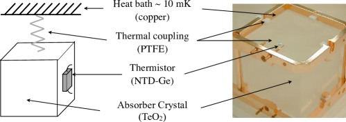
Figure 1: Sketch of a CUORE-like bolometer (left) and a photograph of a bolometer (right). The $\mathrm{TeO}_{2}$ crystal is held by Teflon supports, the thermistor is glued to the crystal and its wires are attached to the copper frame. The supports and the thermistor wires thermally couple the crystal to the copper frame, which act as heat bath.

To read out the signal, the thermistor is biased in differential configuration with a bipolar voltage generator $\pm V_{bias}$ connected to a pair of load resistors, $R_{L}$’s, finally connected to the thermistor’s terminals. The resistance of the thermistor varies in time with the temperature, $R(t)$, and the voltage across it, $V_{R}(t)$, is the bolometer signal. The value of $R_{L}$’s is chosen to be much higher than $R(t)$ so that $V_{R}(t)$ is proportional to $R(t)$. Since from Eq. (1) positive temperature variations induce negative resistance variations, the polarity of $V_{bias}$ is chosen to be negative in order to obtain positive signals. The connecting wires add in parallel to the thermistor a parasitic capacitance $c_{p}$. A schematic of the biasing circuit is shown in Fig. 2. In the figure, the series of the two load resistors is represented as a unique resistor $R_{L}$. The signal $V_{R}(t)$ is amplified, filtered with a 6-pole active Bessel filter, and then digitized with an 18-bit analog-to-digital converter (ADC). To fit the signal in the range of the ADC, which is [-10.5,10.5]$\mathrm{\,V}$, a programmable offset voltage $V_{h}$ is added to $V_{R}(t)$. The front-end electronics, which provide the bias voltage, the load resistors, the amplifier and the offset voltage, are placed outside of the cryostat, at ambient temperature [13].

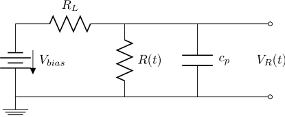
Figure 2: Biasing circuit of the thermistor. A voltage generator $V_{bias}$ biases the thermistor resistance $R(t)$ in series with a load resistance $R_{L}$. The bolometer signal is the voltage $V_{R}(t)$ across $R(t)$. The wires used to extract $V_{R}(t)$ from the cryostat have a non-negligible capacitance $c_{p}$.

At 10$\mathrm{\,mK}$ the value of $R(T)$ is of order $100\mathrm{\,M\mathrm{\,\Omega}}$, $R_{L}$ is chosen as $54\mathrm{\,G\mathrm{\,\Omega}}$ ($27+27\mathrm{\,G\mathrm{\,\Omega}}$) and $V_{bias}$ as $\sim 5$$\mathrm{\,V}$. The $c_{p}$ value depends on the length of the wires that carry the signal out of the cryostat, typically it is of order 400$\mathrm{\,pF}$. The amplifier gain, the Bessel filter frequency bandwidth, the duration of the acquisition window and the sampling frequency are set typically at 5000$\mathrm{\,V/V}$, 12$\mathrm{\,Hz}$, 5.008$\mathrm{\,s}$ and 125$\mathrm{\,Hz}$, respectively.

The data analyzed in this paper come from test bolometers operated by the CUORE collaboration at the Gran Sasso underground laboratory (LNGS) in Italy [14]. The bolometers were exposed to a ²³²Th calibration source which, together with an $\alpha$ line generated by ²¹⁰Po contamination in the crystal, allows the analysis of an energy range up to 5407$\mathrm{\,keV}$.

To simplify the description of this work we will focus our analysis on a single bolometer. The signal rate on that bolometer was 133 mHz, that has to be combined to the rate of heater pulses that were fired at an energy of 1885$\mathrm{\,keV}$ every 300 seconds (3.3 mHz). The energy spectrum acquired in about $3\mathrm{\,days}$ is shown in Fig. 3.

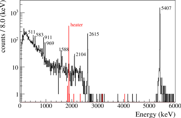
Figure 3: Energy spectrum. All lines are generated by the ${}^{232}\mathrm{Th}$ calibration source except for the line at 5407$\mathrm{\,keV}$, arising from ²¹⁰Po contamination in the $\mathrm{TeO}_{2}$ crystal. Heater pulses were fired at an energy of $1885\mathrm{\,keV}$.

3 Signal and noise features

Examples of signals generated by a 2615$\mathrm{\,keV}$ $\gamma$-ray and by the heater, as acquired by the ADC, are shown in Fig. 4. The baseline voltage of the pulses is related to the thermistor temperature in static conditions, and the amplitude is related to the energy released. The shape of heater pulses is found to be slightly different from that of particle pulses: the rise time of the particle (heater) pulse in the figure, computed as the time difference between the 10% and the 90% of the leading edge, is 55 (54) $\mathrm{\,ms}$ while the decay time, computed as the difference between the 90% and 30% of the trailing edge, is 220 (255) $\mathrm{\,ms}$.

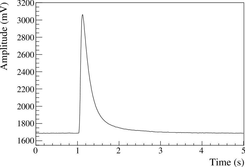
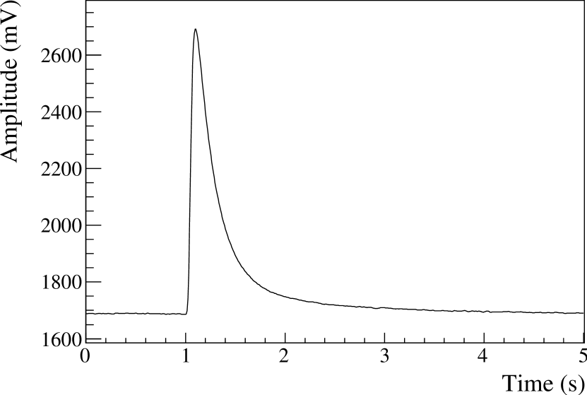
Figure 4: Pulse shapes of a 2615$\mathrm{\,keV}$ $\gamma$-ray (left) and heater (right). The baseline is related to the temperature of the thermistor before the particle interaction or the heater shot. The amplitude carries information on the amount of energy released.

As already observed in Ref. [4] several nonlinearities are present:

1. The rise and the decay times of a pulse depend on the energy (Fig. 5).

   \begin{overpic}[clip={true},width=433.62pt]{fig5a_risetime_std.eps} \put(34.0,20.0){\footnotesize heater} \end{overpic}

   \begin{overpic}[clip={true},width=433.62pt]{fig5b_decaytime_std.eps} \put(42.0,60.0){\footnotesize heater} \end{overpic}

   Figure 5: Pulse shape parameters versus energy. The correlation with energy is negative for the rise time (left) and positive for the decay time (right). Heater pulses are marked in red.

2. The amplitude of the pulse depends on the base temperature, which varies during the data acquisition (Fig. 6).

   

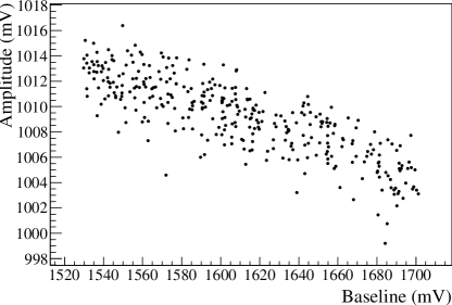
   Figure 6: Amplitude of heater pulses versus baseline. A change in the bolometer temperature also changes its response, degrading the energy resolution.

3. The amplitude dependence on energy is not linear. The deviation from linearity of the data is estimated by comparing the result of a linear calibration function,

   $$\rm{Energy}=\rm{constant}\cdot\rm{Amplitude}\;,$$ (2)

   to the true energy of the source peaks. The residuals evaluated on the peaks generated by the ²³²Th source (see Fig. 3) are shown in Fig. 7. The 5407$\mathrm{\,keV}$ line is not considered here because $\alpha$ particles have a quenching factor different from $\gamma$ and $\beta$ particles [5].

   

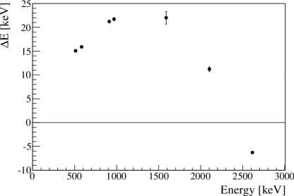
   Figure 7: Residuals obtained using a linear calibration function for the well-identified peaks in the ²³²Th source spectrum. Considering that the energy resolution is $\sim 5\mathrm{\,keV\,FWHM}$, the difference $\Delta E$ between the estimated energies and the true peak energies is not compatible with zero. The error bars refer to the uncertainty on the estimated peak position that depends on the FWHM and on the number of events $N$ in the peak as ${\rm FWHM}/(2.35\sqrt{N})$.

The noise of the bolometer in the signal frequency region (0-10$\mathrm{\,Hz}$) is a result of vibrations inside the cryostat, and depends on the mechanical setup of the experimental apparatus. The noise power spectrum was estimated as:

$$N(\omega_{k})\,=\;<|n(\omega_{k})|^{2}>$$ (3)

where $n(\omega_{k})$ is the k-th component of the discrete Fourier transform (DFT) of an acquired waveform not containing signals, and $<>$ denotes the average over a large number of waveforms. A typical noise waveform and the estimated power spectrum are shown in Fig. 8. The peaks in the power spectrum are due to the crystal friction against its frame, and the residual common mode contribution from the vibration of the connecting wires (readout by the differential preamplifier). Which of the two sources is dominant may depend on the set-up. The white noise contribution at high frequency is due to the ADC digitization.

In the next sections we will describe the procedure we developed to simulate the signal shape, the nonlinearities and the noise.

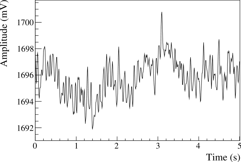
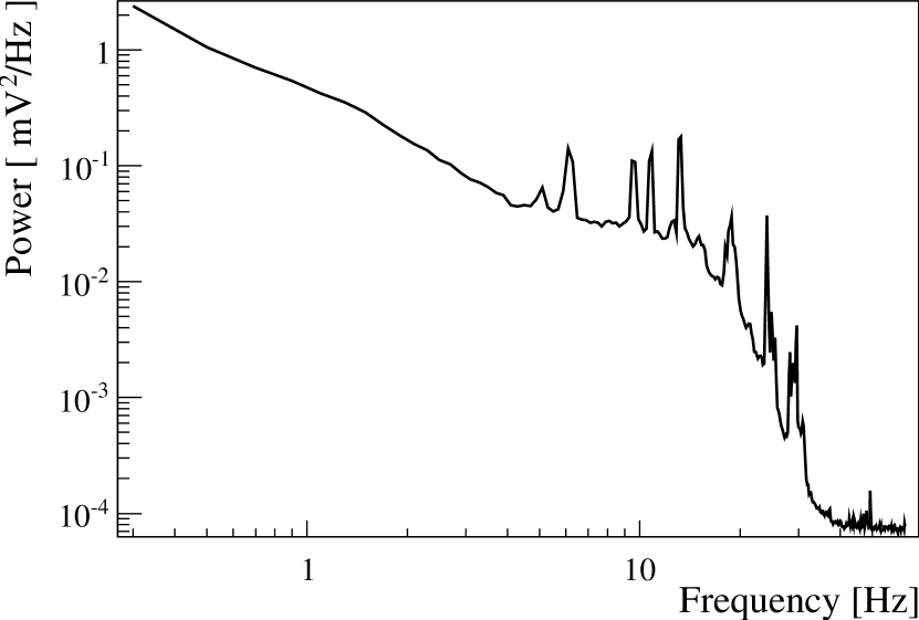
Figure 8: Noise of a bolometer at the output of the acquisition chain. A sample waveform (left) and the power spectrum estimated from a large number of waveforms (right).

4 Signal model

To simulate the data we developed a model of the bolometer signal that reproduces the pulse shape and the nonlinearities. Starting from the energy release in the crystal, the model is divided into three main stages: the thermal response of the bolometer, the response of the thermistor and of its biasing circuit, and the simulation of the electronics. All parameters are detector variables, except for the thermal model parameters, which we determine from fits to the data.

4.1 Thermal model

A bolometer is a thermal system composed of a crystal, crystal supports, thermistor, and their coupling elements [15] (Fig. 9). The crystal capacitance $C_{c}$ is connected to the thermistor through the glue spots with conductance $K_{g}$ and to the supports through a contact conductance $K_{cs}$. The thermistor can be represented as a two-stage system composed of a lattice and an electron gas, each with its capacitance and conductance, and inter-connected by a conductance $K_{ep}$. The lattice capacitance, not shown in the figure, is negligible and it discharges through the gold wires connected to the main heat bath $K_{Au}$. The electron gas capacitance and conductance are labeled as $C_{e}$ and $K_{e}$, respectively. The left side of the circuit shows the crystal supports with their capacitance $C_{s}$ and their conductance to the main bath $K_{s}$. The main bath acts as the reference ground.

Figure 9: Thermal circuit of a CUORE-like bolometer. Each of the elements is identified in the text.

We are interested in the expression of the temperature variation of the thermistor electron gas (node 4 in Fig. 9) as a function of the time $\Delta T(t)$ after that an amount of energy $E$ is released in the crystal. The energy release is effectively instantaneous, because the phonons produced by a particle thermalize in a time much shorter than the rise time of acquired pulses [16]. Under these conditions the analytical expression of $\Delta T(t)$ is found to be:

$$\Delta T(t)=A_{T}\left(-e^{-\frac{t}{\tau_{r}}}+\alpha e^{-\frac{t}{\tau_{d1}}}+(1-\alpha)e^{-\frac{t}{\tau_{d2}}}\right)\;,$$ (4)

where all the parameters are complicated functions of the elements of the thermal circuit. The formula indicates that the thermistor temperature increases with one rise time constant, $\tau_{r}$, and decreases with two decay constants, $\tau_{d1}$ and $\tau_{d2}$. The parameter $\alpha$ weighs the two exponential decays and satisfies the condition $0\leq\alpha\leq 1$. The amplitude of the thermal pulse, $A_{T}$, is also a function of the thermal elements and is directly proportional to $E$.

In principle the parameters in Eq. 4 could be known if one were able to measure the underlying thermal elements. Previous investigators have measured the thermal parameters [15], and obtained heat capacitances and heat conductances of order $10^{-a}\mathrm{\,J/K}$ and $10^{-b}\mathrm{\,W/K}$ with $a$ in the range 9 to 10 and $b$ in the range 9 to 11. Such measurements are of little utility for us for several reasons. First, the capacitances and conductances depend on the temperature and should be measured in the bolometer working temperatures, that depend on the setup. Second, several thermal elements vary from bolometer to bolometer. For example, the contact heat conductance between the crystal and its supports ($K_{cs}$) changes with the detector configuration, and the heat conductance of the glue ($K_{g}$) varies because of the weak reproducibility of the glue deposition. Third, we should know the parameters with a precision of the order of the present energy resolution ($0.1\%$), which is not feasible using ordinary measurements techniques. We choose instead to estimate the parameters in Eq. 4 from fits to the signal waveforms (see Sec. 5).

The solution of the circuit as expressed in Eq. 4 does not include the dependence of the thermal elements on the temperature. This potential source of nonlinearity, however, is not visible in the data [4]. We also neglected the electrothermal feedback effect: when temperature change induces resistance change in a biased thermistor, the resulting excursion in Joule heating induces further temperature change. It can be shown that the electrothermal feedback to the first order acts as a correction to the values of $K_{e}$ and $C_{e}$, and therefore does not affect the configuration of the thermal circuit and the form of Eq. 4.

4.2 Thermistor and biasing circuit models

When the thermistor temperature varies, its resistance varies according to Eq. 1:

$$\Delta R(\Delta T)=R_{0}\exp\left(\frac{T_{0}}{T^{B}+\Delta T}\right)^{\gamma}-R^{B}$$ (5)

where $T^{B}$ is the initial temperature of the bolometer and $R^{B}=R(T^{B})$. Because we do not know the parameters $R_{0}$, $T_{0}$ and $T^{B}$ with the desired accuracy, we adopt an approximation valid for the small $\Delta T$ that will occur [4]:

$$\Delta R(\Delta T)\simeq R^{B}\left[\exp(-\eta\Delta T/T^{B})-1\right]\;,$$ (6)

where

$$\eta=\left|\frac{d\log{R}}{d\log T}\right|={\gamma}\,\log\frac{R(T)}{R_{0}}\;.$$ (7)

$\eta$ is the sensitivity of the thermistor, which has value of order 10 but is not known with precision. The advantage of Eq. 6 is that the parameter $R^{B}$ can be measured with precision and that the unknown $\eta/T^{B}$ is just a scale factor applicable to the temperature variation. We obtain the expression for the resistance variation after an energy release by substituting Eq. 4 into Eq. 6 :

$$\Delta R(t)=R^{B}\;\left\{\exp\Big{[}{-A\left(-e^{-\frac{t}{\tau_{r}}}+\alpha e^{-\frac{t}{\tau_{d1}}}+(1-\alpha)e^{-\frac{t}{\tau_{d2}}}\right)}\Big{]}-1\right\}$$ (8)

where $A=\eta A_{T}/T^{B}$. This expression absorbs the unknown parameter $\eta/T^{B}$ with the unknown thermal amplitude $A_{T}$. The thermistor model therefore does not change the number of unknown parameters and adds the measurable parameter $R^{B}$.

The relationship between the voltage across the thermistor $V_{R}(t)$ and its resistance $R(t)$ can be obtained from the differential equation describing the thermistor’s biasing circuit (see Fig. 2):

$$\bigg{[}\frac{R_{L}+R(t)}{R(t)}\bigg{]}V_{R}(t)-V_{bias}+R_{L}c_{p}\frac{dV_{R}(t)}{dt}=0\;.$$ (9)

The model we are building is based on variations of the resistance from the measured value of $R^{B}$, which in turn generate voltage variations from the corresponding voltage $V_{R}^{B}$:

$$V_{R}^{B}=V_{bias}\frac{R^{B}}{R^{B}+R_{L}}\;.$$ (10)

By splitting $R(t)$ and $V_{R}(t)$ into time-independent and time-dependent contributions,

$$R(t)=R^{B}+\Delta R(t)\quad V_{R}(t)=V^{B}_{R}+\Delta V_{R}(t)\;,$$ (11)

we obtain the differential equation relating resistance and voltage variations:

$$\Bigg{[}\frac{R_{L}+R^{B}+\Delta R(t)}{R^{B}+\Delta R(t)}\Bigg{]}\Bigg{[}V_{bias}\frac{R^{B}}{R^{B}+R_{L}}+\Delta V_{R}(t)\Bigg{]}-V_{bias}+R_{L}c_{p}\frac{d\Delta V_{R}(t)}{dt}=0\;.$$ (12)

Given the form of $\Delta R(t)$ in Eq. 8, $\Delta V_{R}(t)$ cannot be obtained in an closed form. In our bolometer model we solve Eq. 12 numerically using the Runge-Kutta method [17].

The thermistor and the biasing circuit are the only sources of nonlinearities of our model, and should be able to describe the nonlinearities observed in the data. If we assume that the thermal circuit responds linearly, the amplitude $A$ in Eq. 8 is directly proportional to the energy $E$ released in the bolometer,

$$A=c\cdot E\;.$$ (13)

The corresponding resistance variation, however, is not proportional to $A$, because the exponential dependency in Eq. 8 does not transform linearly the shape and the amplitude of the pulse. Moreover the voltage variation is not strictly proportional to the resistance variation. This model description should be sufficient to generate the shape dependence on energy and the nonlinear calibration function (Figs. 5 and 7). The amplitude dependence on the baseline in Fig. 6 can be generated from Eq. 8 by varying the baseline voltage of the pulse and hence the thermistor resistance $R^{B}$.

4.3 Electronics

The front-end electronics amplifies the bolometer signal $\Delta V_{R}(t)$ by $G$, a parameter that is measured with a precision better than $0.2\%$. The deviation from linearity of the amplifier, in the voltage range we are considering, is less than $0.01\%$. The output voltage of the amplifier

$$\Delta V_{G}(t)=\Delta V_{R}(t)\cdot G\;,$$ (14)

is fed into a six-pole Bessel filter, whose transfer function is

$$B(\sigma)=\frac{10395}{\sigma^{6}+21\sigma^{5}+210\sigma^{4}+1260\sigma^{3}+4725\sigma^{2}+10395\sigma+10395}\;.$$ (15)

In the above equation $\sigma$ is the normalized Laplace variable which can be expressed in terms of the frequency $\omega$ as:

$$\sigma=\jmath\omega\frac{2.703395061}{f_{b}}\,,$$ (16)

where $f_{b}$ is the filter cutoff (12$\mathrm{\,Hz}$ in our case).

The signal is filtered by multiplying its DFT, $\Delta V_{G}(\omega)$, by $B(\omega)$, removing the “DFT wraparound problem” with the method described in Ref. [18]. The output of the filter is then obtained as:

$$\Delta V(t)={\cal F}^{-1}[\Delta V_{G}(\omega)\cdot B(\omega)]\;,$$ (17)

where ${\cal F}^{-1}$ denotes the inverse DFT.

In summary , the model of the signal, from the energy release in the crystal $E$ to the signal acquired by the ADC $\Delta V(t)$, is obtained using the thermal model in Eq. 4, the thermistor model in Eq. 8, the voltage across the thermistor from Eq. 12, the amplifier and Bessel filter effects in Eqns. 14 and 17:

$$\Delta V(t)=\left\{\left[E\xrightarrow[\begin{subarray}{c}Eq:~{}\ref{eq:thermal_pulse}\\ {\rm analytic}\\ {\rm solution}\end{subarray}]{}\Delta T(t)\xrightarrow[\begin{subarray}{c}Eq.~{}\ref{eq:thermistor_pulse}\\ {\rm analytic}\\ {\rm solution}\end{subarray}]{}\Delta R(t)\xrightarrow[\begin{subarray}{c}Eq.~{}\ref{eq:voltage_pulse}\\ {\rm numerical\phantom{y}}\\ {\rm solution}\end{subarray}]{}\Delta V_{R}(t)\right]\underset{Eq.~{}\ref{eq:amplifier}}{\cdot}G\right\}\underset{\begin{subarray}{c}{Eq.~{}\ref{eq:bessel_conv}}\\ {\rm DFT}\\ {\rm convolution}\end{subarray}}{\otimes}B(t)\;.$$ (18)

The baseline voltage of the signal, $V^{B}$, is the sum of two components, the thermistor voltage $V^{B}_{R}$ in Eq. 10 scaled by the electronics gain $G$, and the offset voltage $V_{h}$ added by the electronics itself:

$$V^{B}=V_{R}^{B}\cdot G+V_{h}=V_{bias}G\frac{R^{B}}{R^{B}+R_{L}}+V_{h}\;.$$ (19)

To reproduce a real waveform, $V(t)$, we add the baseline voltage to the pulse in Eq. 18 and we also account for the onset time $t_{0}$ of the pulse, which starts about $1\mathrm{\,s}$ after the beginning of the waveform:

$$V(t)=V^{B}+\Theta(t-t_{0})\Delta V(t-t_{0})\;,$$ (20)

where $\Theta(t)$ is the Heaviside step function. Since the thermistor temperature is not stable, the resistance $R^{B}$ and the baseline voltage $V^{B}$ are not fixed parameters of the model. $V^{B}$ is measured on data by averaging the first 0.8$\mathrm{\,s}$ of the waveform. The corresponding value of $R^{B}$ is then computed from Eq. 19 and used in the signal model. In Tab. 1 we list the parameters of the model and indicate whether they are measured, or determined from fits to signal waveforms.

Table 1: Parameters of the signal model in Eqns. 18, 19 and 20.

Parameter	Name	Equation	Estimation
$\tau_{r}$	Thermal rise time	4	Fit
$\alpha$	Weight of the two thermal decay constants	4	Fit
$\tau_{d1}$	Fast thermal decay constant	4	Fit
$\tau_{d2}$	Slow thermal decay constant	4	Fit
$c$	Energy to thermal amplitude conversion	13	Fit
$R^{B}$	Thermistor resistance at the pulse baseline	8	Measured
$V_{bias}$	Bias voltage	12	Measured
$R_{L}$	Load resistor	12	Measured
$c_{p}$	Parasitic capacitance	12	Measured
$G$	Electronics gain	14	Measured
$f_{b}$	Bessel filter cutoff frequency	17	Measured
$V_{h}$	Electronics offset voltage	19	Measured
$V^{B}$	Baseline voltage	20	Measured
$t_{0}$	Onset time of the pulse	20	Fit

5 Estimation of the signal model

We intend that the model we developed accounts for all the nonlinearities of the signal. The unknown thermal parameters in Tab. 1 are expected to be independent of the energy, except for the amplitude $A$, which should be proportional to the energy (Eq. 13). The energy independence allows us to determine unmeasured parameters from fits to pulses at a single energy, and apply the resulting model over the entire range of energies. We performed fits on particle pulses occurring in an energy window of 30$\mathrm{\,keV}$ around the 2615$\mathrm{\,keV}$ $\gamma$ peak. We performed a separate set of fits on heater pulses, because their shape differs from the shape of particle pulses.

Figure 10 shows a typical fit to a 2615$\mathrm{\,keV}$$\gamma$-ray pulse, Tab. 2 reports the parameters averaged over 25 fits of particle and heater pulses.

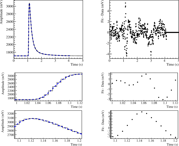
Figure 10: Fit of a 2615$\mathrm{\,keV}$ pulse. Data (black solid lines) with superimposed fit function (Eq. 20) (blue dashed lines) are shown in the left column, fit residuals are shown in the right column. The two bottom rows display a zoom of the rise and of the maximum of the pulse, respectively. The fit region ends when the pulse falls to within 3 standard deviations of the baseline level.

Table 2: Average parameters fitted on particle (2615$\mathrm{\,keV}$ $\gamma$) and heater pulses and the $\chi^{2}/{\rm ndf}$ of the fits.

Parameter	Particle	Heater
$\tau_{r}\;\mathrm{\,(ms)}$	$20.70\pm 0.05$	$18.8\pm 0.1$
$\alpha\;$	$0.916\pm 0.002$	$0.911\pm 0.002$
$\tau_{d1}\;\mathrm{\,(ms)}$	$158.1\pm 0.5$	$187.3\pm 0.6$
$\tau_{d2}\;\mathrm{\,(ms)}$	$770\pm 20$	$970\pm 20$
$c\;\mathrm{\,(1/MeV)}$	$0.04703\pm 0.00006$	$0.04356\pm 0.00009$
$t_{0}\;\mathrm{\,(s)}$	$1.0145\pm 0.0005$	$0.9944\pm 0.0005$
$\chi^{2}/{\rm ndf}\;$	$2.4\pm 0.3$	$2.0\pm 0.2$

The average $\chi^{2}$ is about twice the number of degrees of freedom, i.e. about twice the value one expects for a perfect model. Shortcomings of the model are also apparent in the fit residuals on the right of the figure, where mismatches are evident in the leading edge and in the vicinity of the maximum of the pulse. The voltage amplitude of the fit function is slightly biased, and found to be, on average, higher than the amplitude of the pulse by $0.17\pm 0.02\mathrm{\,\%}$ for particle pulses and $0.37\pm 0.02\mathrm{\,\%}$ for particle heater pulses.

The fit error can be ascribed to an incompleteness of the thermal model, that would probably benefit from the inclusion of second order effects like the nonlinearities of the thermal elements and the electrothermal feedback. For our purposes, however, the model performs well, reproducing the signal at the per mil level.

6 Noise generation

A complete and predictive model for the noise of CUORE bolometers is missing. The main sources of fluctuations that spoil the energy resolution have different origins and, to estimate the overall contribution, each of them should be propagated with the transfer function of each step of the acquisition chain. Examples of these sources are the Johnson noise of the load resistors, vibrations of the experimental apparatus that dissipate energy in the bolometer and instabilities of the cryostat temperature. All these effects contribute to the power spectrum shown in Fig. 8.

Although the noise from the load resistors and amplifiers is predictable, a model for the noise from vibrations is not in hand. Moreover, it varies from bolometer to bolometer, because of the weak reproducibility of the assembly. On this account we adopted a statistical model for the noise. We simply require that, on average, the simulated time series behave like the experimental one, namely that the average power spectrum of the simulated baselines is as close as possible to data.

We followed an approach [19] based on an application of the Carson’s theorem [20] to a discrete time series. A random waveform $n(t_{i})$ can be represented as a superposition of independent pulses of fixed shape $g(t_{i})$ and amplitude $A$, distributed in time according to a Poisson process of rate $\lambda$:

$$n(t_{i})=A\,\sum_{l}g(t_{i}-t_{l})\;,$$ (21)

where the differences between consecutive $t_{l}$’s follow an exponential distribution with mean $1/\lambda$. The theorem states that $N(\omega_{k})$ and $G(\omega_{k})$, the average power spectra of $n(t_{i})$ and $g(t_{i})$, respectively (see Eq. 3), satisfy the relationship:

$$N(\omega_{k})=\lambda TA^{2}G(\omega_{k})\;,$$ (22)

where $T$ is the length of the time series (5.008$\mathrm{\,s}$ in our case). To utilize the theorem one must find a shape $g(t_{i})$ for which the power spectrum is proportional to the average power spectrum of the noise time series to be simulated. $A^{2}$ and $\lambda$ are adjustable parameters with product fixed by Eq. 22. These parameters set the aspect of the noise in the time domain, i.e. the same power spectrum can be produced with a small rate of pulses with large amplitude and vice versa. Once $g(t_{i})$ and, say, $\lambda$ are determined the method is fully specified and $n(t_{i})$ is obtained from Eq. 21.

We built $g(t_{i})$ as the inverse DFT of

$$g(\omega_{k})=\sqrt{N(\omega_{k})}e^{\jmath\theta_{k}}\;,$$ (23)

where $\theta_{k}$ is a phase randomly sampled within $[0,2\pi]$. The reality of $g(t_{i})$ is guaranteed by imposing the constraint $g(\omega_{k})=g^{*}(-\omega_{k})$. $\lambda$ was chosen equal to the Nyquist frequency (62.5$\mathrm{\,Hz}$), i.e. the maximum rate producing distinguishable pulses.

The left panel of Fig. 11 shows a simulated and a measured noise waveform, and their appeareance is similar. The right panel of the figure shows the agreement between simulated and measured power spectra.

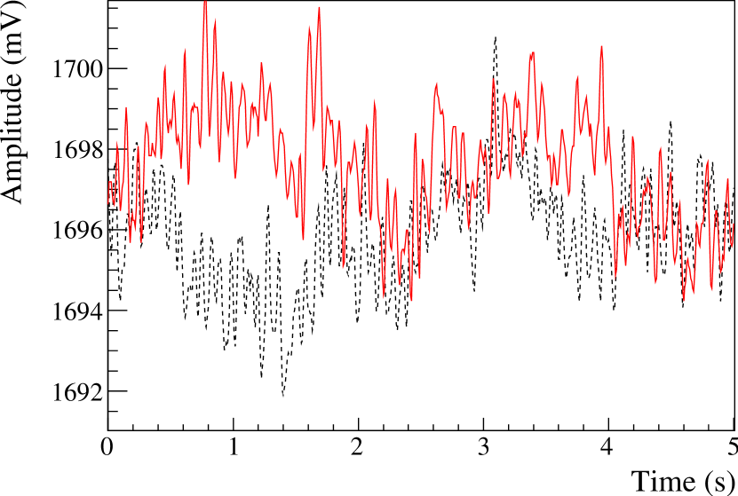
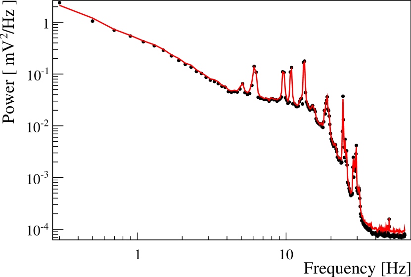
Figure 11: Comparison of noise simulation (solid red line) with data (dashed black line / dots). Sample waveforms (left) and the power spectrum estimated from a large number of waveforms (right).

7 Simulation and validation with data

We built a simulation engine that is able to generate particle, heater, and pure noise waveforms. It uses as input the parameters of the signal model in Tab. 1 and the measured noise power spectrum. To correct the small error of the model in reproducing the pulse shape (see Sec. 5), the engine scales the simulated signals by the estimated bias, so as to match the amplitude of measured signals. The simulated noise is summed to the signal assuming that it is purely additive. The additivity is supported by the fact that the absolute energy resolution for heater pulses is independent of the energy release, and by the residuals in Fig. 10 that do not seem correlated with the time evolution of the pulse.

The simulation can be highly customized. One can choose the energy distribution of the events to be generated, the baseline distribution, and the distribution of the time interval between events. The features of the signal described in Sec. 3 should be automatically reproduced by the model, and signals close in time are summed to reproduce pileups.

To validate the simulation engine, we show the results of a simulation configured to reproduce the data shown in Sec. 3. Signals were generated sampling their energy from the spectrum in Fig. 3, the baseline was generated in the range of Fig. 6, the time delay between particle pulses was generated following an exponential distribution with mean $1/(133\mathrm{\,mHz})$, and heater pulses were generated every 300$\mathrm{\,s}$. Particle and heater pulses were generated using the fitted parameters in Tab. 2, and the noise was generated from the power spectrum in Fig. 8.

The comparison of the simulation with the data shows good agreement. The shape of the pulses with noise added reproduces well the acquired waveforms (Fig. 12). The distributions of the rise and decay times shown in Fig. 13 also confirm the agreement. We attribute a small mismatch in the rise time of heater pulses to imperfections of the model (see Sec. 5). The correlation between pulse amplitude and baseline is very well reproduced (Fig. 14). The dependence of amplitude on energy follows the data well at high energies (Fig. 15). The mismatch of order 1% at zero energy is another manifestation of the imperfections of the model. In most applications this error is ignorable, nonetheless we incorporated an option to generate waveforms by sampling from the amplitude spectrum instead of the energy spectrum, in which case the mismatch is suppressed by fiat.

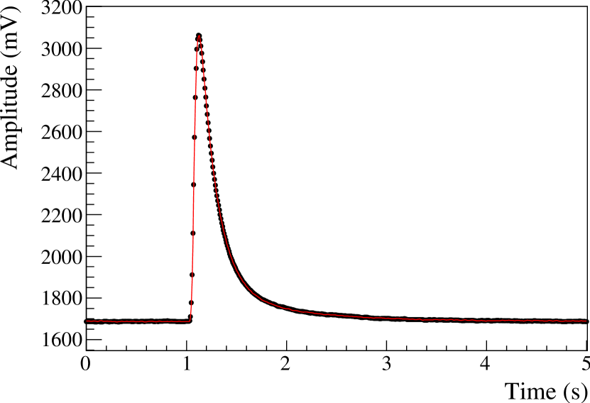
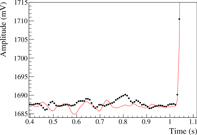
Figure 12: Comparison of the simulation (solid red line) of a 2615$\mathrm{\,keV}$ $\gamma$ pulse with data (black dots). Full waveform (left) and expansion of the leading edge of the signal (right).

\begin{overpic}[clip={true},width=433.62pt]{fig13a_risetime_std_mc.eps} \put(34.0,20.0){\footnotesize heater} \end{overpic}

\begin{overpic}[clip={true},width=433.62pt]{fig13b_decaytime_std_mc.eps} \put(42.0,60.0){\footnotesize heater} \end{overpic}

Figure 13: Comparison of the rise time (left) and decay time (right). The black, gray, red, and blue dots represent measured particle pulses, simulated particle pulses, measured heater pulses, and simulated heater pulses respectively.

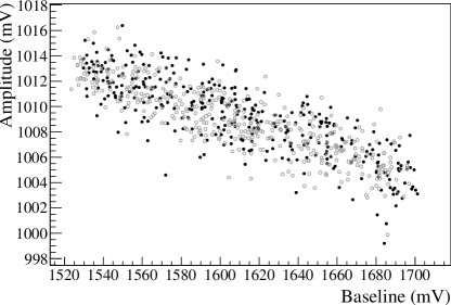
Figure 14: Comparison of the amplitude of heater pulses versus baseline from data (solid black) and simulation (open gray).

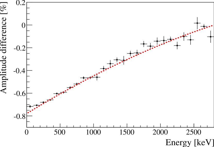
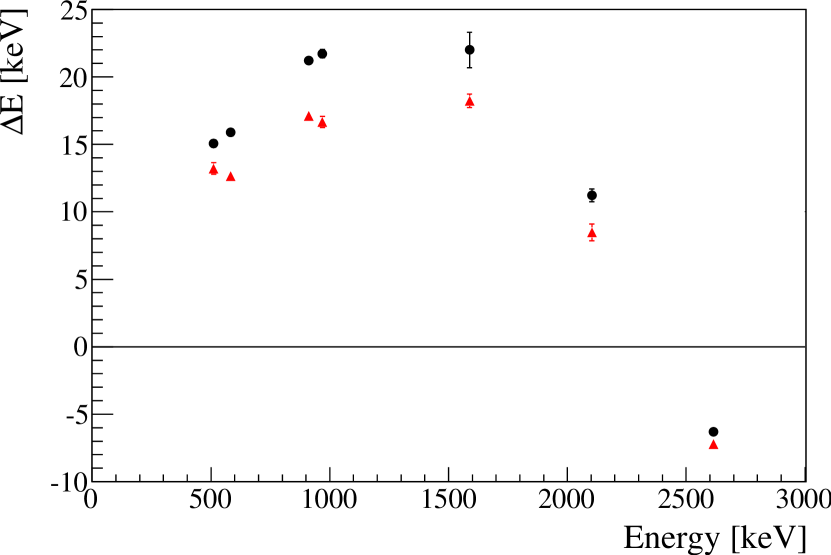
Figure 15: Difference between the amplitudes of simulated and real pulses as a function of the energy (left), and deviation from linearity of the calibration function (right) for data (black circles) and simulation (red triangles).

8 Applications

The simulation can be used to test and tune analysis algorithms, comparing the results with the so called “Monte Carlo truth”, i.e. the generated values of baseline, amplitude, energy and the time of each signal. In same cases, in fact, the signal identification is not straightforward and the energy could be wrongly estimated.

For example the data analysis can be complicated by pileups, that alter the baseline and the shape of the signals. A simulated sequence of close signals is shown in Fig. 16, where it can be seen how a signal can be modified by other signals, and how its identification is complicated. In this case the simulation can be used to improve the analysis algorithms and to estimate the error on the results.

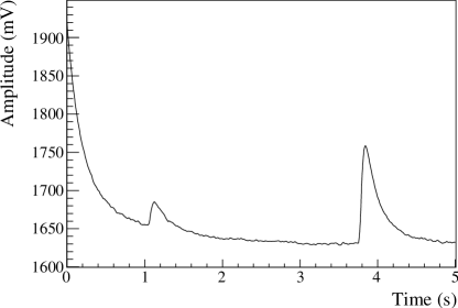
Figure 16: Simulated pileups. The pulse at $\sim 1\mathrm{\,s}$ was generated with an energy of 63$\mathrm{\,keV}$, lies on the tail of a previous pulse of 1899$\mathrm{\,keV}$ and is succeeded by a pulse of 263$\mathrm{\,keV}$.

A potential application is the estimation of detection efficiencies at low energy. Recently it has been demonstrated [3] that CUORE may have an energy threshold of only a few keV, thus being sensitive to Dark Matter interactions and rare nuclear decays. Figure 17 shows simulations of very small pulses. In this regime noise can both mask signal and mimic signal. Simulations produced by our engine may be used to test the immunity of analysis algorithms to both types of error. When a heater is available it is used to produce controlled pulses and estimate the detection efficiencies. The simulation can correct for the difference in pulse shape between particle and heater generated energy deposit. With no heater the simulation could serve on its own to estimate the detection efficiencies.

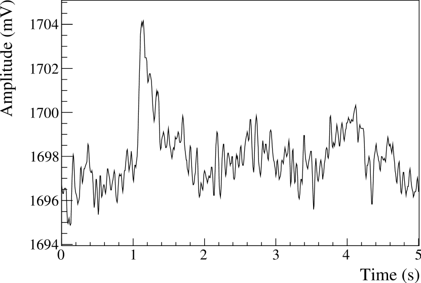
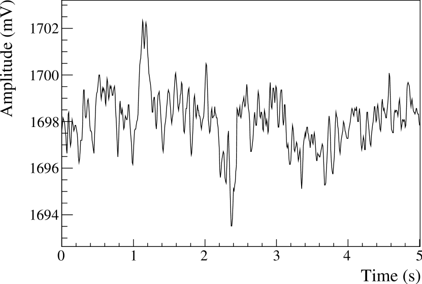
Figure 17: 12$\mathrm{\,keV}$ (left) and 6$\mathrm{\,keV}$ (right) simulated pulses.

- [1] R. Ardito et. al., CUORE: A cryogenic underground observatory for rare events, arXiv:hep-ex/0501010 (2005) [hep-ex/0501010].
- [2] C. Arnaboldi et. al., CUORE: A Cryogenic Underground Observatory for Rare Events, Nucl. Instr. Meth. in Phys. Res. A. 518 (2004) 775, [hep-ex/0212053v1].
- [3] S. Di Domizio, F. Orio, and M. Vignati, Lowering the energy threshold of large-mass bolometric detectors, JINST 6 (2011) P02007, [arXiv:1012.1263].
- [4] M. Vignati, Model of the Response Function of Large Mass Bolometric Detectors, J.Appl.Phys. 108 (2010) 084903, [arXiv:1006.4043].
- [5] F. Bellini et. al., Response of a bolometer to alpha particles, JINST 5 (2010) P12005, [arXiv:1010.2618].
- [6] N. Wang, F. C. Wellstood, B. Sadoulet, E. E. Haller, and J. Beeman, Electrical and thermal properties of neutron-transmutation-doped Ge at 20 mK, Phys. Rev. B 41 (1990), no. 6 3761.
- [7] K. M. Itoh et. al., Neutron transmutation doping of isotopically engineered Ge, Appl. Phys. Lett. 64 (1994) 2121.
- [8] A. Alessandrello et. al., Methods for response stabilization in bolometers for rare decays, Nucl. Instr. Meth. in Phys. Res. A. (1998), no. 412 454.
- [9] C. Arnaboldi, G. Pessina, and E. Previtali, A programmable calibrating pulse generator with multi- outputs and very high stability, IEEE Trans. Nucl. Sci. 50 (2003) 979.
- [10] N. F. Mott, Localized states in a pseudogap and near extremities of conduction and valence bands, Phil. Mag. 19 (1969) 835.
- [11] A. Efros and B. Shklovskii, Electronic properties of doped semiconductors, p. 202. Springer-Verlag, Berlin, 1984.
- [12] K. M. Itoh et. al., Hopping conduction and metal-insulator transition in isotopically enriched neutron-transmutation-doped 70Ge:Ga, Phys. Rev. Lett. 77 (1996), no. 19 4058.
- [13] C. Arnaboldi et. al., The programmable front-end system for CUORICINO, an array of large-mass bolometers, IEEE Trans. Nucl. Sci. 49 (2002) 2440.
- [14] C. Arnaboldi et. al., Production of high purity TeO2 single crystals for the study of neutrinoless double beta decay, J. Cryst. Growth 312 (2010), no. 20 2999.
- [15] A. Alessandrello et. al., An Electrothermal Model for Large Mass Bolometric Detectors, IEEE Trans. Nucl. Sci. 40 (1993), no. 4 649.
- [16] F. Pröbst et. al., Model for cryogenic particle detectors with superconducting phase transition thermometers, J. Low. Temp. Phys. 100 (1995) 69–104.
- [17] M. Abramowitz and I. A. Stegun, Handbook of Mathematical Functions with Formulas, Graphs, and Mathematical Tables. Dover, New York, ninth dover printing, tenth gpo printing ed., 1964.
- [18] W. H. Press, S. A. Teukolsky, W. T. Vetterling, and B. P. Flannery, Numerical recipes in C (2nd ed.): the art of scientific computing. Cambridge University Press, New York, NY, USA, 1992.
- [19] M. Carrettoni and O. Cremonesi, Generation of noise time series with arbitrary power spectrum, Comput. Phys. Commun. 181 (2010), no. 12 1982.
- [20] J. Carson, The Statistical Energy-Frequency Spectrum of Random Disturbances, Bell Syst. Techn. J. 10 (1931) 374.