The Tsallis Distribution and Transverse Momentum Distributions in High-Energy Physics.

Abstract

The Tsallis distribution has been used recently to fit the transverse momentum distributions of identified particles by the STAR collaboration Abelev:2006cs at the Relativistic Heavy Ion Collider and by the ALICE Aamodt:2011zj and CMS Khachatryan:2011tm collaborations at the Large Hadron Collider. Theoretical issues are clarified concerning the thermodynamic consistency of the Tsallis distribution in the particular case of relativistic high energy quantum distributions. An improved form is proposed for describing the transverse momentum distribution and fits are presented together with estimates of the parameter $q$ and the temperature $T$.

I Introduction

The Tsallis distribution has gained prominence recently in high energy physics with very high quality fits of the transverse momentum distributions made by the STAR collaboration Abelev:2006cs at the Relativistic Heavy Ion Collider and by the ALICE Aamodt:2011zj and CMS Khachatryan:2011tm collaborations at the Large Hadron Collider.

In the literature there exists more than one version of the Tsallis distribution Tsallis:1987eu ; Tsallis:1998ab and we would like to investigate in this paper one version which we consider suited for describing results in high energy particle physics. Our main guiding criterium will be thermodynamic consistency which has not always been implemented correctly (see e.g. Pereira:2007hp ; Pereira:2009ja ; Conroy:2010wt ). The explicit form which we use for the transverse momentum distribution in relativistic heavy ion collisions is:

$$\frac{dN}{dp_{T}~{}dy}=$$

$$gV\frac{p_{T}m_{T}\cosh y}{(2\pi)^{2}}\left[1+(q-1)\frac{m_{T}\cosh y-\mu}{T}\right]^{q/(1-q)},$$ (1)

where $p_{T}$ and $m_{T}$ are the transverse momentum and mass respectively, $y$ is the rapidity, $T$ and $\mu$ are the temperature and the chemical potential, the other variables are defined below. In the limit where the parameter $q$ goes to 1 this reproduces the standard Boltzmann distribution:

$$\lim_{q\rightarrow 1}\frac{dN}{dp_{T}~{}dy}=$$

$$gV\frac{p_{T}m_{T}\cosh y}{(2\pi)^{2}}\exp\left(-\frac{m_{T}\cosh y-\mu}{T}\right).$$ (2)

In order to distinguish Eq. (1) from the form used by the ALICE and CMS collaborations Aamodt:2011zj ; Khachatryan:2011tm we will refer to Eq. (1) as the Tsallis-B parameterization. Note in particular the extra power of $q$ on the right hand side. The motivation for preferring this form is presented in detail in the rest of this paper, see in particular section VII.

Thermal models have been successful in describing particle yields at different beam energies Cleymans:2005xv ; Andronic:2005yp ; Becattini:2005xt , especially in heavy ion collisions. These models assume the formation of a system which is in thermal and chemical equilibrium in the hadronic phase and are characterized by a set of thermodynamic variables for the hadronic phase, most important among these are the chemical freeze-out temperature and baryon chemical potential. The deconfined period of the time evolution dominated by quarks and gluons remains hidden: full equilibration generally washes out and destroys large amounts of information about the early deconfined phase.

While the description of integrated particle yields is reasonably successful, more detailed descriptions, especially of the transverse and longitudinal momentum distributions call for additional dynamics. The transverse momentum distribution is often described by a combination of transverse flow and a thermodynamical statistical distribution. With the Tsallis distribution this superposition is not used and a very good fit can be obtained using the additional parameter $q$ which describes the deviation from a Boltzmann distribution. In the limit where $q\rightarrow 1$ one recovers the standard statistical Boltzmann distribution. Whether this is ultimately the correct description or not remains to be seen. This paper is a contribution to the understanding of the use of the Tsallis distribution in high energy collisions. It is not meant as giving a final answer to the correct dynamical theory of heavy ion collisions.
In the next section we review the derivation of the Tsallis distribution by emphasizing the quantum statistical form and the thermodynamic consistency.

II Tsallis Distribution for Particle Multiplicities.

Several generalizations of the standard Fermi-Dirac distribution

$$n^{FD}(E)\equiv\frac{1}{1+\exp\left(\frac{E-\mu}{T}\right)}.$$ (3)

to a Tsallis form have been proposed in the literature, some of these have been shown not to be thermodynamically consistent. In the following we use the Tsallis form of Fermi-Dirac distribution proposed in turkey1 ; Pennini1995309 ; Teweldeberhan:2005wq ; Conroy:2008uy ; Conroy:2010wt which uses

$$n^{FD}_{T}(E)\equiv\frac{1}{1+\exp_{q}\left(\frac{E-\mu}{T}\right)}.$$ (4)

where the function $\exp_{q}(x)$ is defined as

$$\exp_{q}(x)\equiv\left\{\begin{array}[]{l l}\left[1+(q-1)x\right]^{1/(q-1)}&~{}~{}\mathrm{if}~{}~{}~{}x>0\\ \left[1+(1-q)x\right]^{1/(1-q)}&~{}~{}\mathrm{if}~{}~{}~{}x\leq 0\\ \end{array}\right.$$ (5)

and, in the limit where $q\rightarrow 1$ reduces to the standard exponential:

$$\lim_{q\rightarrow 1}\exp_{q}(x)\rightarrow\exp(x)$$

The form given in Eqs. (4) and (5) will be referred to as the Tsallis-FD distribution. The Bose-Einstein version (given below) will be referred to as the Tsallis-BE distribution Chen200265 while the Boltzmann approximation will be referred to as Tsallis-B distribution. It should be noted that variations of the above have been presented previously in the literature. These will not be considered in this paper.

As is well-known, all forms of the Tsallis distribution introduce a new parameter $q$. In practice this parameter is always close to 1, e.g. in the results obtained by the ALICE and CMS collaborations typical values for the parameter $q$ can be obtained from fits to the transverse momentum distribution for identified charged particles  Aamodt:2011zj and are close to the value 1.1 (see below). The value of $q$ should thus be considered as never being far from 1, deviating from it by 20% at most. An analysis of the composition of final state particles leads to a similar result Cleymans:2008mt for the parameter $q$.

In the limit where $q\rightarrow 1$ the two forms coincide. Numerically the difference is small, as shown in Fig. (1) for a value of $q=1.1$.

The Boltzmann approximation leads to the result Tsallis:1987eu ; Tsallis:1998ab

$$n_{T}^{B}(E)=\left[1+(q-1)\frac{E-\mu}{T}\right]^{-\frac{1}{q-1}}.$$ (6)

Note that we do not use the normalized $q$-probabilities which have been proposed in Ref. Tsallis:1998ab since we use here mean occupation numbers which do not need to be normalized. In the limit where $q\rightarrow 1$ all distributions coincide with the standard statistical distributions:

$$\lim_{q\rightarrow 1}n_{T}^{B}(E) = n^{B}(E),$$ (7)

$$\lim_{q\rightarrow 1}n_{T}^{FD}(E) = n^{FD}(E),$$ (8)

$$\lim_{q\rightarrow 1}n_{T}^{BE}(E) = n^{BE}(E).$$ (9)

A derivation of the Tsallis distribution, based on the Boltzmann equation, has been given in Ref. Biro:2005uv . A comparison between the $n_{T}^{FD}$ and $n^{FD}$ distributions is shown in Fig. (1). For the Boltzmann approximation, the Tsallis distribution is always larger than the Boltzmann one if $q>1$. Taking into account the large $p_{T}$ results for particle production we will only consider this possibility in this paper. As a consequence, in order to keep the particle yields the same, the Tsallis distribution always leads to smaller values of the freeze-out temperature for the same set of particle yields Cleymans:2008mt .

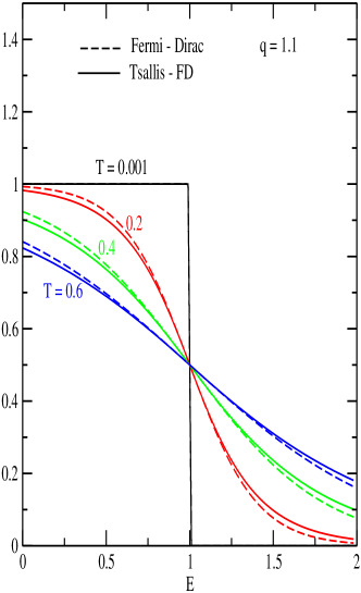
Figure 1: Comparison between the Fermi-Dirac and Tsallis-FD distributions as a function of the energy $E$, keeping the Tsallis parameter $q$ fixed, for various values of the temperature $T$. The chemical potential is kept equal to one in all curves, the units are arbitrary.

The Tsallis distribution for quantum statistics has been considered in Ref. Teweldeberhan:2002wv ; Plastino:2004ge ; turkey1 ; Pennini1995309 ; Chen200265 .

III Thermodynamic Consistency

The first and second laws of thermodynamics lead to the following two differential relations deGroot:1980aa

$$d\epsilon=Tds+\mu dn,$$ (10)

$$dP=sdT+nd\mu.$$ (11)

where $\epsilon=E/V$, $s=S/V$ and $n=N/V$. Since these are total differentials, thermodynamic consistency requires that the following relations be satisfied

$$T = \left.\frac{\partial\epsilon}{\partial s}\right|_{n},$$ (12)

$$\mu = \left.\frac{\partial\epsilon}{\partial n}\right|_{s},$$ (13)

$$n = \left.\frac{\partial P}{\partial\mu}\right|_{T},$$ (14)

$$s = \left.\frac{\partial P}{\partial T}\right|_{\mu}.$$ (15)

The pressure, energy density and entropy density are all given by corresponding integrals over Tsallis distributions and the derivatives have to reproduce the corresponding physical quantities. For completeness, in the next section, we derive Tsallis thermodynamics using the maximal entropy principle and discuss quantum $q$-statistics in particular Bose-Einstein and Fermi-Dirac distribution by maximizing the entropy of the system for quantum distributions. This follows partly the derivation of Ref. Conroy:2010wt . We will show that the consistency conditions given above are indeed obeyed by the Tsallis-FD distribution.

IV Quantum Statistics

The entropy in standard statistical mechanics for fermions is given in the large volume limit by:

$$S^{FD}=-gV \displaystyle\int\frac{d^{3}p}{(2\pi)^{3}}\left[n^{FD}\ln n^{FD}\right.$$ (16)

$$+\left.(1-n^{FD})\ln(1-n^{FD})\right],$$

where $g$ is the degeneracy factor and $V$ the volume of the system. For simplicity Eq. (16) refers to one particle species but can be easily generalized to many by summing over all of them. In the limit where momenta are quantized, which is given by:

$$S^{FD}=-g\displaystyle\sum_{i}\left[n_{i}\ln n_{i}+(1-n_{i})\ln(1-n_{i})\right],$$ (17)

For convenience we will work with the discrete form in the rest of this section. The large volume limit can be recovered with the standard replacement:

$$\sum_{i}\rightarrow V\displaystyle\int\frac{d^{3}p}{(2\pi)^{3}}$$ (18)

The generalization, using the Tsallis prescription, leads to turkey1 ; Pennini1995309 ; Teweldeberhan:2005wq

$$S^{FD}_{T}=-g\displaystyle\sum_{i}\left[n_{i}^{q}\ln_{q}n_{i}+(1-n_{i})^{q}\ln_{q}(1-n_{i})\right],$$ (19)

where use has been made of the function

$$\ln_{q}(x)\equiv\frac{x^{1-q}-1}{1-q},$$ (20)

often referred to as q-logarithm. It can be easily shown that in the limit where the Tsallis parameter $q$ tends to 1 one has:

$$\lim_{q\rightarrow 1}\ln_{q}(x)=\ln(x).$$ (21)

The maximization of the entropy (19) will give the $n_{i}$’s their Tsallis-type form. If we use the explicit form of the “q-logarithms” we obtain

$$S^{FD}_{T}=g\displaystyle\sum_{i}\left[\left(\frac{n_{i}-n_{i}^{q}}{q-1}\right)+\left(\frac{(1-n_{i})-(1-n_{i})^{q}}{q-1}\right)\right],$$ (22)

In a similar vein, the generalized form of the entropy for bosons is given by

$$S^{BE}_{T}=-g\displaystyle\sum_{i}\left[n_{i}^{q}\ln_{q}n_{i}-(1+n_{i})^{q}\ln_{q}(1+n_{i})\right],$$ (23)

by using a similar method, we can express equation (23) as

$$S^{BE}_{T}=g\displaystyle\sum_{i}\left[\left(\frac{n_{i}-n_{i}^{q}}{q-1}\right)-\left(\frac{(1+n_{i})-(1+n_{i})^{q}}{q-1}\right)\right],$$ (24)

In the limit $q\rightarrow 1$ equations (19) and (23) reduce to the standard Fermi-Dirac and Bose-Einstein distributions. Further, as we shall presently explain, the formulation of a variational principle in terms of equation (22) allows to prove the general relation of thermodynamics. One of the relevant constraints is given by the average number of particles,

$$\sum_{i}n_{i}^{q}=N.$$ (25)

Notice the unusual power of $q$ on the left-hand side. As it turns out, it is necessary to have this power of $q$ since otherwise there is no thermodynamic consistency.

Likewise, the energy of the system gives a constraint,

$$\sum_{i}n_{i}^{q}E_{i}=E.$$ (26)

again, it is necessary to have the power $q$ on the left-hand side as no thermodynamic consistency would be achieved without it. The maximization of the entropic measure equation (22) under the constraints equation (25) and (26) leads to the variational problem.

$$\frac{\delta}{\delta n_{i}}\left[S^{FD}_{T}+\alpha(N-\displaystyle\sum_{i}n_{i}^{q})+\beta(E-\displaystyle\sum_{i}n_{i}^{q}E_{i})\right]=0,$$ (27)

where $\alpha$ and $\beta$ are Lagrange multipliers associated, respectively, with the total number of particles and the total energy. Differentiating each expression in equation (27)

$$\frac{\delta}{\delta n_{i}}\left(S^{FD}_{T}\right)=\frac{q}{q-1}\left[\left(\frac{1-n_{i}}{n_{i}}\right)^{q-1}-1\right]n_{i}^{q-1},$$ (28)

$$\frac{\delta}{\delta n_{i}}\left(N-\displaystyle\sum_{i}n_{i}^{q}\right)=-qn_{i}^{q-1},$$ (29)

and

$$\frac{\delta}{\delta n_{i}}\left(E-\displaystyle\sum_{i}n_{i}^{q}E_{i}\right)=-qE_{i}n_{i}^{q-1},$$ (30)

then by substituting equation (28), (29) and (30) into (27), we obtain

$$qn_{i}^{q-1}\left\{\frac{1}{q-1}\left[-1+\left(\frac{1-n_{i}}{n_{i}}\right)^{q-1}\right]-\beta E_{i}-\alpha\right\}=0.$$ (31)

which can be rewritten as

$$\frac{1}{q-1}\left[-1+\left(\frac{1-n_{i}}{n_{i}}\right)^{q-1}\right]=\beta E_{i}+\alpha,$$ (32)

and, by rearranging equation (32), we get

$$\frac{1-n_{i}}{n_{i}}=\left[1+(q-1)(\beta E_{i}+\alpha)\right]^{\frac{1}{q-1}},$$

finally, we get the solution of generalized form of Fermi-Dirac distribution like this

$$n_{i} = \frac{1}{\left[1+(q-1)(\beta E_{i}+\alpha)\right]^{\frac{1}{q-1}}+1},$$ (33)

$$= \frac{1}{\left[\exp_{q}(\alpha+\beta E_{i})\right]+1},$$

Which is the expression for the Tsallis-FD distribution referred to earlier in this paper turkey1 ; Pennini1995309 ; Teweldeberhan:2005wq .

Using a similar approach one can also determine the Tsallis-BE distribution Chen200265 . Starting from the extremum of the entropy subject to two conditions one has:

$$\frac{\delta}{\delta n_{i}}\left[S^{BE}_{T}+\alpha(N-\displaystyle\sum_{i}n_{i}^{q})+\beta(E-\displaystyle\sum_{i}n_{i}^{q}E_{i})\right]=0,$$ (34)

which leads to

$$\frac{\delta}{\delta n_{i}}\left(S^{BE}_{T}\right)=\frac{q}{q-1}\left[\left(\frac{1+n_{i}}{n_{i}}\right)^{q-1}-1\right]n_{i}^{q-1},$$ (35)

and by using equations (35),(29) and (30) in (34), one gets

$$\sum_{i}qn_{i}^{q-1}\left\{\frac{1}{q-1}\left[-1+\left(\frac{1+n_{i}}{n_{i}}\right)^{q-1}\right]-\beta E_{i}-\alpha\right\}=0.$$ (36)

By rearranging equation (36), one obtains the expression for the Tsallis-BE distribution Chen200265 ,

$$n_{i} = \frac{1}{\left[1+(q-1)(\beta E_{i}+\alpha)\right]^{\frac{1}{q-1}}-1},$$ (37)

$$= \frac{1}{\left[\exp_{q}((E_{i}-\mu)/T)\right]-1}.$$

where the usual identifications $\alpha=-\mu/T$ and $\beta=1/T$ have been made.

V Proof of Thermodynamical Consistency

In order to use the above expressions it has to be shown that they satisfy the thermodynamic consistency conditions. To show this in detail we use the first law of thermodynamics deGroot:1980aa

$$P=\frac{-E+TS+\mu N}{V},$$ (38)

and take the partial derivative with respect to $\mu$ in order to check for thermodynamic consistency, it leads to

$$\left.\frac{\partial P}{\partial\mu}\right|_{T} = \frac{1}{V}\left[-\frac{\partial E}{\partial\mu}+T\frac{\partial S}{\partial\mu}+N+\mu\frac{\partial N}{\partial\mu}\right],$$ (39)

$$= \frac{1}{V}\left[N+\displaystyle\sum_{i}-\frac{T}{q-1}\left(1+(q-1)\frac{E_{i}-\mu}{T}\right)\frac{\partial n_{i}^{q}}{\partial\mu}\right.$$

$$\left.+\frac{Tq(1-n_{i})^{q-1}}{q-1}\frac{\partial n_{i}}{\partial\mu}\right],$$

then, by explicit calculation

$$\frac{\partial n_{i}^{q}}{\partial\mu}=\frac{qn_{i}^{q+1}}{T}\left[1+(q-1)\frac{E_{i}-\mu}{T}\right]^{-1+\frac{1}{1-q}},$$

$$\frac{\partial n_{i}}{\partial\mu}=\frac{n_{i}^{2}}{T}\left[1+(q-1)\frac{E_{i}-\mu}{T}\right]^{-1+\frac{1}{1-q}},$$

and

$$\left(1-n_{i}\right)^{q-1}=n_{i}^{q-1}\left[1+\frac{(q-1)(E_{i}-\mu)}{T}\right].$$

Introducing this into equation (39), yields

$$\left.\frac{\partial P}{\partial\mu}\right|_{T}=n,$$ (40)

which proves the thermodynamical consistency (14).

We also calculate explicitly the relation in equation (12) can be rewritten as

$$\left.\frac{\partial E}{\partial S}\right|_{n} =\frac{\frac{\partial E}{\partial T}dT+\frac{\partial E}{\partial\mu}d\mu}{\frac{\partial S}{\partial T}dT+\frac{\partial S}{\partial\mu}d\mu},$$

$$=\frac{\frac{\partial E}{\partial T}+\frac{\partial E}{\partial\mu}\frac{d\mu}{dT}}{\frac{\partial S}{\partial T}+\frac{\partial S}{\partial\mu}\frac{d\mu}{dT}},$$ (41)

since $n$ is kept fixed one has the additional constraint

$$dn=\frac{\partial n}{\partial T}dT+\frac{\partial n}{\partial\mu}d\mu=0,$$

leading to

$$\frac{d\mu}{dT}=-\frac{\frac{\partial n}{\partial T}}{\frac{\partial n}{\partial\mu}}.$$ (42)

Now, we rewrite (V) and (42) in terms of the following expressions

$$\frac{\partial E}{\partial T}=\displaystyle\sum_{i}qE_{i}n_{i}^{q-1}\frac{\partial n_{i}}{\partial T},$$

$$\frac{\partial E}{\partial\mu}=\displaystyle\sum_{i}qE_{i}n_{i}^{q-1}\frac{\partial n_{i}}{\partial\mu},$$

$$\frac{\partial S}{\partial T}=\displaystyle\sum_{i}q\left[\frac{-n_{i}^{q-1}+(1-n_{i})^{q-1}}{q-1}\right]\frac{\partial n_{i}}{\partial T},$$

$$\frac{\partial S}{\partial\mu}=\displaystyle\sum_{i}q\left[\frac{-n_{i}^{q-1}+(1-n_{i})^{q-1}}{q-1}\right]\frac{\partial n_{i}}{\partial\mu},$$

$$\frac{\partial n}{\partial T}=\frac{1}{V}\left[\displaystyle\sum_{i}qn_{i}^{q-1}\frac{\partial n_{i}}{\partial T}\right],$$

and

$$\frac{\partial n}{\partial\mu}=\frac{1}{V}\left[\displaystyle\sum_{i}qn_{i}^{q-1}\frac{\partial n_{i}}{\partial\mu}\right].$$

By introducing the above relations into equation (V), the numerator of equation (V) becomes

$$\frac{\partial E}{\partial T} + \frac{\partial E}{\partial\mu}\frac{d\mu}{dT}=\displaystyle\sum_{i}qE_{i}n_{i}^{q-1}\frac{\partial n_{i}}{\partial T}$$ (43)

$$-\frac{\displaystyle\sum_{i,j}q^{2}E_{j}\left(n_{i}n_{j}\right)^{q-1}\frac{\partial n_{j}}{\partial\mu}\frac{\partial n_{i}}{\partial T}}{\displaystyle\sum_{j}qn_{j}^{q-1}\frac{\partial n_{j}}{\partial\mu}},$$

$$= \frac{\displaystyle\sum_{i,j}qE_{i}\left(n_{i}n_{j}\right)^{q-1}C_{ij}}{\displaystyle\sum_{j}n_{j}^{q-1}\frac{\partial n_{j}}{\partial\mu}}.$$

Where the abbreviation

$$C_{ij}\equiv\left(n_{i}n_{j}\right)^{q-1}\left[\frac{\partial n_{i}}{\partial T}\frac{\partial n_{j}}{\partial\mu}-\frac{\partial n_{j}}{\partial T}\frac{\partial n_{i}}{\partial\mu}\right],$$ (44)

has been introduced. One can rewrite the denominator part of equation (V) as

$$\frac{\partial S}{\partial T}+\frac{\partial S}{\partial\mu}\frac{d\mu}{dT} =\frac{\displaystyle q\sum_{i,j}\left[{-n_{i}^{q-1}+(1-n_{i})^{q-1}}\right]n_{j}^{q-1}C_{i,j}}{(q-1)\displaystyle\sum_{j}n_{j}^{q-1}\frac{\partial n_{j}}{\partial\mu}},$$

$$=\frac{\displaystyle q\sum_{i,j}(E_{i}-\mu)\left(n_{i}n_{j}\right)^{q-1}C_{i,j}}{T\displaystyle\sum_{j}n_{j}^{q-1}\frac{\partial n_{j}}{\partial\mu}},$$ (45)

where

$$\frac{-n_{i}^{q-1}+(1-n_{i})^{q-1}}{q-1}=\frac{(E_{i}-\mu)}{T}n_{i}^{q-1},$$

hence, by substituting equation (43) and (V) in to (V), we find

$$\left.\frac{\partial E}{\partial S}\right|_{n}=T\frac{\displaystyle\sum_{i,j}E_{i}C_{ij}}{\displaystyle\sum_{i,j}(E_{i}-\mu)C_{ij}},$$ (46)

since $\displaystyle\sum_{i,j}C_{ij}=0$, this finally leads to the desired result

$$\left.\frac{\partial E}{\partial S}\right|_{n}=T.$$ (47)

Hence thermodynamic consistency is satisfied.

VI Boltzmann Approximation

Due to its practical relevance and importance we devote a section to the Tsallis-B distribution. In this case the entropy is obtained from equation (15) by assuming the $n_{i}\ll 1$, this leads to

$$S_{T}^{B}\equiv g\displaystyle\sum_{i=1}^{W}\frac{(n_{i}-n_{i}^{q})}{q-1}+n_{i},$$ (48)

The $n_{i}$ are given explicitly as

$${n}_{i}=\left[1+(q-1)\frac{E_{i}-\mu}{T}\right]^{\frac{1}{1-q}},$$ (49)

where $n_{i}$ denotes the number of particles in the $i$th energy level with energy $E_{i}$. The maximum of the above entropy is looked for under the constraints imposed by fixing the total number of particles $N$ and the total energy of the system $E$, as given in equation (25) and (26). As in the previous section, it should satisfy thermodynamic consistency which is given in equation (12). The derivative of pressure w.r.t. $\mu$ becomes

$$\left.\frac{\partial P}{\partial\mu}\right|_{T} =\frac{1}{V}\left[-\frac{\partial E}{\partial\mu}+T\frac{\partial S}{\partial\mu}+N+\mu\frac{\partial N}{\partial\mu}\right],$$

$$=\frac{1}{V}\left[N+\displaystyle\sum_{i}-\frac{Tn_{i}^{1-q}}{q-1}\frac{\partial n_{i}^{q}}{\partial\mu}+\frac{Tq}{q-1}\frac{\partial n_{i}}{\partial\mu},\right],$$ (50)

now, by using

$$\frac{\partial n_{i}^{q}}{\partial\mu}=qn_{i}^{q-1}\frac{\partial n_{i}}{\partial\mu},$$

and

$$\frac{\partial n_{i}}{\partial\mu}=\frac{n_{i}^{q}}{T}.$$

By the above relations in equation (VI), we recover equation (14).

We now calculate the expressions needed in equations (V) and (42) in terms of

$$\frac{\partial S}{\partial T}=\displaystyle\sum_{i}\left[1+\frac{1-qn_{i}^{q-1}}{q-1}\right]\frac{\partial n_{i}}{\partial T},$$

$$\frac{\partial S}{\partial\mu}=\displaystyle\sum_{i}\left[1+\frac{1-qn_{i}^{q-1}}{q-1}\right]\frac{\partial n_{i}}{\partial\mu},$$

while the other partial derivatives are the same as previously. by plugging the above relations into equation (V), then the numerator part of equation (V) become

$$\frac{\partial E}{\partial T}+\frac{\partial E}{\partial\mu}\frac{d\mu}{dT} = \displaystyle\sum_{i}qE_{i}n_{i}^{q-1}\frac{\partial n_{i}}{\partial T}$$ (51)

$$-\frac{\displaystyle\sum_{i,j}q^{2}E_{j}\left(n_{i}n_{j}\right)^{q-1}\frac{\partial n_{j}}{\partial\mu}\frac{\partial n_{i}}{\partial T}}{\displaystyle\sum_{j}qn_{j}^{q-1}\frac{\partial n_{j}}{\partial\mu}},$$

$$= \frac{\displaystyle\sum_{i,j}qE_{i}\left(n_{i}n_{j}\right)^{q-1}C_{i,j}}{\displaystyle\sum_{j}n_{j}^{q-1}\frac{\partial n_{j}}{\partial\mu}}.$$

Similarly, the denominator part of equation (V) can be written as

$$\frac{\partial S}{\partial T} + \frac{\partial S}{\partial\mu}\frac{d\mu}{dT}=\displaystyle\sum_{i}\left[1+\frac{1-qn_{i}^{q-1}}{q-1}\right]\frac{\partial n_{i}}{\partial T}$$ (52)

$$-\frac{\displaystyle\sum_{i,j}n_{i}^{q-1}\left[1+\frac{1-qn_{j}^{q-1}}{q-1}\right]\frac{\partial n_{j}}{\partial\mu}\frac{\partial n_{i}}{\partial T}}{\displaystyle\sum_{j}n_{j}^{q-1}\frac{\partial n_{j}}{\partial\mu}},$$

$$= \frac{\displaystyle\sum_{i,j}\left[1+\frac{1-qn_{i}^{q-1}}{q-1}\right]n_{j}^{q-1}C_{i,j}}{\displaystyle\sum_{j}n_{j}^{q-1}\frac{\partial n_{j}}{\partial\mu}},$$

$$= \frac{\displaystyle\sum_{i,j}\frac{q(E_{i}-\mu)}{T}\left(n_{i}n_{j}\right)^{q-1}C_{i,j}}{\displaystyle\sum_{j}n_{j}^{q-1}\frac{\partial n_{j}}{\partial\mu}},$$

where

$$1+\frac{1-qn_{i}^{q-1}}{q-1}=\frac{q(E_{i}-\mu)}{T}n_{i}^{q-1},$$

by combining the expressions in equation (51) and (52) into (V), we find as before

$$\left.\frac{\partial E}{\partial S}\right|_{n}=T.$$ (53)

It has thus been shown that the definitions of temperature and pressure within the Tsallis formalism for non-extensive thermostatistics lead to expressions which satisfy consistency with the first law of thermodynamics.

VII Thermal Fit Details

The total number of particles is given by the integral version of (25),

$$N=gV\displaystyle\int\frac{d^{3}p}{(2\pi)^{3}}\left[1+(q-1)\frac{E-\mu}{T}\right]^{q/(1-q)},$$ (54)

The extra power of $q$ is necessary for thermodynamic consistency. The corresponding (invariant) momentum distribution is given by

$$E\frac{dN}{d^{3}p}=gVE\frac{1}{(2\pi)^{3}}\left[1+(q-1)\frac{E-\mu}{T}\right]^{q/(1-q)},$$ (55)

which, in terms of the rapidity and transverse mass variables, becomes

$$\frac{dN}{dy\,m_{T}dm_{T}} = gV\frac{m_{T}\cosh y}{(2\pi)^{2}}$$ (56)

$$\times\left[1+(q-1)\frac{m_{T}\cosh y-\mu}{T}\right]^{q/(1-q)},$$

At mid-rapidity $y=0$ and for zero chemical potential this reduces to the following expression

$$\left.\frac{dN}{m_{T}dm_{T}~{}dy}\right|_{y=0}=gV\frac{m_{T}}{(2\pi)^{2}}\left[1+(q-1)\frac{m_{T}}{T}\right]^{q/(1-q)},$$ (57)

or, introducing the transverse momentum:

$$\left.\frac{dN}{dp_{T}~{}dy}\right|_{y=0}=gV\frac{p_{T}m_{T}}{(2\pi)^{2}}\left[1+(q-1)\frac{m_{T}}{T}\right]^{q/(1-q)}.$$ (58)

Fits using the above expressions based on the Tsallis-B distribution to experimental measurements published by the CMS collaboration Khachatryan:2011tm are shown in Figs. 2, 3 and 4 and are comparable with those shown by the CMS collaboration but the resulting parameters are considerably different and are collected in Table I. The most striking feature is that the values of the parameter $q$ are fairly stable around the value $q\approx 1.11$ for all cases considered, whether 7 Tev or 0.9 TeV. The same cannot be said about the temperature $T$ which is around 100 MeV with considerable deviations, it is however well below the values quoted by the CMS collaboration Khachatryan:2011tm . The analytic expression used in Refs. Aamodt:2011zj ; Khachatryan:2011tm corresponds to identifying

$$n\rightarrow\frac{q}{q-1}$$ (59)

an additional factor of the transverse mass on the right-hand side and a shift in the mass.

Particle	$T$ (MeV)	$q$
$K^{0}_{S}$ (0.9 TeV)	92	1.13
$K^{0}_{S}$ (7 TeV)	105	1.15
$\Lambda$ (0.9 TeV)	70	1.11
$\Lambda$ (7 TeV)	117	1.12
$\Xi^{-}$ (0.9 TeV)	44	1.11
$\Xi^{-}$ (7 TeV)	126	1.11

Table 1: Fitted values of the $T$ and $q$ parameters for strange particles measured by the CMS collaboration Khachatryan:2011tm using the Tsallis-B form for the momentum distribution. The normalization has been adjusted.

VIII Conclusions

In this paper we have presented a detailed derivation of the quantum form of the Tsallis distribution and considered in detail the thermodynamic consistency of the resulting distribution. It was emphasized that an additional power of $q$ is needed to achieve consistency with the laws of thermodynamics Conroy:2010wt . The resulting distribution, called Tsallis-B, was compared with recent measurements from the CMS collaboration Khachatryan:2011tm and good agreement was obtained. The resulting parameter $q$ which is a measure for the deviation from a standard Boltzmann distribution was found to be around 1.11. The resulting values of the temperature show a wider spread around 100 MeV.

Whether or not the Tsallis distribution provides a valid interpretation of high energy collision data will need further theoretical work.

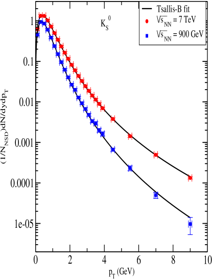
Figure 2: Comparison between the measured transverse momentum distribution for $K^{0}_{S}$ as measured by the CMS collaboration Khachatryan:2011tm and the Tsallis-B distribution as given by Eq. (57) using the parameters listed in Table I.

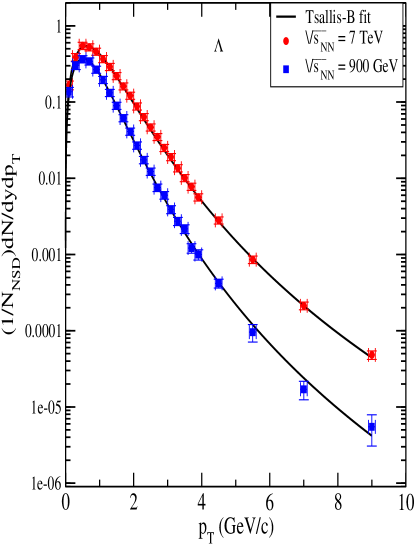
Figure 3: Comparison between the measured transverse momentum distribution for $\Lambda$ as measured by the CMS collaboration Khachatryan:2011tm and the Tsallis-B distribution as given by Eq. (57) using the parameters listed in Table I.

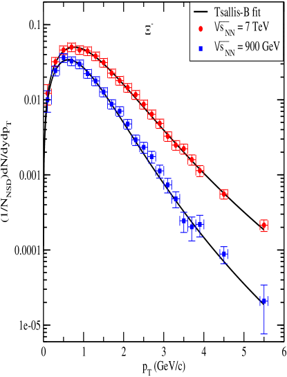
Figure 4: Comparison between the measured transverse momentum distribution for $\Lambda$ as measured by the CMS collaboration Khachatryan:2011tm and the Tsallis-B distribution as given by Eq. (57) using the parameters listed in Table I.

References

- (1) B. I. Abelev et al. (STAR), Phys. Rev. C75, 064901 (2007), arXiv:nucl-ex/0607033
- (2) K. Aamodt et al. (ALICE Collaboration)(2011), arXiv:1101.4110 [hep-ex]
- (3) V. Khachatryan et al. (CMS), JHEP 05, 064 (2011), arXiv:1102.4282 [hep-ex]
- (4) C. Tsallis, J.Statist.Phys. 52, 479 (1988)
- (5) C. Tsallis, R. S. Mendes, and A. R. Plastino, Physica A261, 534 (1998)
- (6) F. Pereira, R. Silva, and J. Alcaniz, Phys.Rev. C76, 015201 (2007), arXiv:0705.0300 [nucl-th]
- (7) F. Pereira, R. Silva, and J. Alcaniz, Phys.Lett. A373, 4214 (2009), arXiv:0906.2422 [nucl-th]
- (8) J. M. Conroy, H. G. Miller, and A. R. Plastino, Phys.Lett. A374, 4581 (2010), arXiv:1006.3963 [cond-mat.stat-mech]
- (9) J. Cleymans, H. Oeschler, K. Redlich, and S. Wheaton, Phys. Rev. C73, 034905 (2006), arXiv:hep-ph/0511094
- (10) A. Andronic, P. Braun-Munzinger, and J. Stachel, Nucl. Phys. A772, 167 (2006), arXiv:nucl-th/0511071
- (11) F. Becattini, J. Manninen, and M. Gazdzicki, Phys.Rev. C73, 044905 (2006), arXiv:0511092 [hep-ph]
- (12) F. Buyukkilic and D. Demirhan, Phys.Lett. A181, 24 (1993)
- (13) F. Pennini, A. Plastino, and A. R. Plastino, Physics Letters A 208, 309 (1995)
- (14) A. M. Teweldeberhan, A. R. Plastino, and H. G. Miller, Phys.Lett. A343, 71 (2004)
- (15) J. M. Conroy and H. Miller, Phys.Rev. D78, 054010 (2008), arXiv:0801.0360 [hep-ph]
- (16) J. Chen, Z. Zhang, G. Su, L. Chen, and Y. Shu, Physics Letters A 300, 65 (2002)
- (17) J. Cleymans, G. Hamar, P. Levai, and S. Wheaton, J.Phys. G36, 064018 (2009), arXiv:0812.1471 [hep-ph]
- (18) T. Biro and G. Purcsel, Phys.Rev.Lett. 95, 162302 (2005), arXiv:hep-ph/0503204 [hep-ph]
- (19) A. Teweldeberhan, H. Miller, and R. Tegen, Int.J.Mod.Phys. E12, 395 (2003), arXiv:0210011 [hep-ph]
- (20) A. Plastino, A. Plastino, H. Miller, and H. Uys, Astrophys.Space Sci. 290, 275 (2004)
- (21) S. R. de Groot, W. A. van Leeuwen, and C. G. van Weert, Relativistic Kinetic Theory (North Holland, 1980)