HANDLING UNCERTAINTIES IN SVM CLASSIFICATION

Abstract

This paper addresses the pattern classification problem arising when available target data include some uncertainty information. Target data considered here is either qualitative (a class label) or quantitative (an estimation of the posterior probability). Our main contribution is a SVM inspired formulation of this problem allowing to take into account class label through a hinge loss as well as probability estimates using $\varepsilon$-insensitive cost function together with a minimum norm (maximum margin) objective. This formulation shows a dual form leading to a quadratic problem and allows the use of a representer theorem and associated kernel. The solution provided can be used for both decision and posterior probability estimation. Based on empirical evidence our method outperforms regular SVM in terms of probability predictions and classification performances.

Index Terms—  support vector machines, maximal margin algorithm, uncertain labels.

1 Introduction

In the mainstream supervised classification scheme, an expert is required for labelling a set of data used then as inputs for training the classifier. However, even for an expert, this labeling task is likely to be difficult in many applications. In the end the training data set may contain inaccurate classes for some examples, which leads to non robust classifiers[1]. For instance, this is often the case in medical imaging where radiologists have to outline what they think are malignant tissues over medical images without access to the reference histopatologic information. We propose to deal with these uncertainties by introducing probabilistic labels in the learning stage so as to: 1. stick to the real life annotation problem, 2. avoid discarding uncertain data, 3. balance the influence of uncertain data in the classification process.
Our study focuses on the widely used Support Vector Machines (SVM) two-class classification problem [2]. This method aims a finding the separating hyperplane maximizing the margin between the examples of both classes. Several mappings from SVM scores to class membership probabilities have been proposed in the literature [3, 4]. In our approach, we propose to use both labels and probabilities as input thus learning simultaneously a classifier and a probabilistic output. Note that the output of our classifier may be transformed to probability estimations without using any mapping algorithm.
In section 2 we define our new SVM problem formulation (referred to as P-SVM) to deal with certain and probabilistic labels simultaneously. Section 3 describes the whole framework of P-SVM and presents the associated quadratic problem. Finally, in section 5 we compare its performances to the classical SVM formulation (C-SVM) over different data sets to demonstrate its potential.

2 Problem formulation

We present below a new formulation for the two-class classification problem dealing with uncertain labels. Let $X$ be a feature space. We define $(x_{i},l_{i})_{i=1\dots m}$ the learning dataset of input vectors $(x_{i})_{i=1\dots m}\in X$ along with their corresponding labels $(l_{i})_{i=1\dots m}$, the latter of which being

• class labels: $l_{i}$ = $y_{i}\in\{-1,+1\}$ for $i=1\dots n$ (in classification),

• real values: $l_{i}$ = $p_{i}\in[0,1]$ for $i=n+1\dots m$ (in regression).

$p_{i}$, associated to point $x_{i}$ allows to consider uncertainties about point $x_{i}$’s class. We define it as the posterior probability for class 1.

$p_{i}=p(x_{i})=\mathbb{P}(Y_{i}=1\mid X_{i}=x_{i})$.

We define the associated pattern recognition problem as

$$\vspace*{-0.2cm}\displaystyle\min_{w} \quad\frac{1}{2}\|w\|^{2}$$ (1)

subject to $$\begin{cases}y_{i}(w^{\top}x_{i}+b)\geq 1,&i=1...n\\ z_{i}^{-}\leq w^{\top}x_{i}+b\leq z_{i}^{+},&i=n+1...m\vspace*{-0.2cm}\end{cases}$$

Where boundaries $z_{i}^{-}$, $z_{i}^{+}$ directly depend on $p_{i}$. This formulation consists in minimizing the complexity of the model while forcing good classification and good probability estimation (close to $p_{i}$). Obviously, if $n=m$, we are brought back to the classical SVM problem formulation.

Following the idea of soft margin introduced in regular SVM to deal with the case of inseparable data, we introduce slack variables $\xi_{i}$. This measure the degree of misclassification of the datum $x_{i}$ thus relaxing hard constraints of the initial optimization problem which becomes

$$\vspace*{-0.2cm}\displaystyle\min_{w,\xi,\xi^{-},\xi^{+}}\frac{1}{2}\|w\|^{2}+C\displaystyle\sum\limits_{i=1}^{n}\xi_{i}+\tilde{C}\displaystyle\sum\limits_{i=n+1}^{m}(\xi^{-}_{i}+\xi^{+}_{i})$$ (2)

subject to

$$\begin{cases}y_{i}(w^{\top}x_{i}+b)\geq 1-\xi_{i},&i=1...n\\ z_{i}^{-}-\xi^{-}_{i}\leq w^{\top}x_{i}+b\leq z_{i}^{+}+\xi^{+}_{i},&i=n+1...m\\ 0\leq\xi_{i},&i=1...n\\ 0\leq\xi_{i}^{-}\mbox{ and }0\leq\xi_{i}^{+},&i=n+1...m\\ \end{cases}$$

Parameters $C$ and $\tilde{C}$ are predefined positive real numbers controlling the relative weighting of classification and regression performances.
Let $\varepsilon$ be the labelling precision and $\delta$ the confidence we have in the labelling. Let’s define $\eta$ = $\varepsilon$ + $\delta$. Then, the regression problem consists in finding optimal parameters $w$ and $b$ such that

$\mid\frac{1}{\displaystyle 1+e^{-a(w^{\top}x_{i}+b)}}-p_{i}\mid<\eta$ ,

Thus constraining the probability prediction for point $x_{i}$ to remain around to $\frac{1}{1+e^{-a(w^{\top}x_{i}+b)}}$ within distance $\eta$ [5, 6, 7]. The boundaries (where $w^{\top}x_{i}+b=\pm 1$), define parameter $a$ as:

$a=\ln(\frac{1}{\eta}-1)$

Finally: $\max(0,p_{i}-\eta)$ $\leq$ $\frac{1}{\displaystyle 1+e^{-a(w^{\top}x_{i}+b)}}$ $<$ $\min(p_{i}+\eta,1)$, $\Longleftrightarrow$ $z_{i}^{-}$ $\leq$ $w^{\top}x_{i}+b$ $<$ $z_{i}^{+}$,

where $z_{i}^{-}=-\frac{1}{a}\ln(\frac{1}{p_{i}-\eta}-1)$ and $z_{i}^{+}=-\frac{1}{a}\ln(\frac{1}{p_{i}+\eta}-1)$.

3 Dual formulation

We can rewrite the problem in its dual form, introducing Lagrange multipliers. We are looking for a stationary point for the Lagrange function $L$ defined as

$\textit{L}(w,b,\xi,\xi^{-},\xi^{+},\alpha,\beta,\mu^{+},\mu^{-},\gamma^{+},\gamma^{-})=$

$$\begin{array}[]{ll}&\frac{1}{2}\|w\|^{2}+C\displaystyle\sum\limits_{i=1}^{n}\xi_{i}+\tilde{C}\displaystyle\sum\limits_{i=n+1}^{m}(\xi^{-}_{i}+\xi^{+}_{i})\\ &-\displaystyle\sum\limits_{i=1}^{n}\alpha_{i}(y_{i}(w^{\top}x_{i}+b)-(1-\xi_{i}))-\displaystyle\sum\limits_{i=1}^{n}\beta_{i}\xi_{i}\\ &-\displaystyle\sum\limits_{i=n+1}^{m}\mu_{i}^{-}((w^{\top}x_{i}+b)-(z_{i}^{-}-\xi_{i}^{-}))-\displaystyle\sum\limits_{i=n+1}^{m}\gamma_{i}^{-}\xi_{i}^{-}\\ &-\displaystyle\sum\limits_{i=n+1}^{m}\mu_{i}^{+}((z_{i}^{+}+\xi_{i}^{+})-(w^{\top}x_{i}+b))-\displaystyle\sum\limits_{i=n+1}^{m}\gamma^{+}_{i}\xi_{i}^{+}\\ \end{array}$$

with $\alpha\geq 0$, $\beta\geq 0$, $\mu^{+}\geq 0$, $\mu^{-}\geq 0$,$\gamma^{+}\geq 0$ and $\gamma^{-}\geq 0$
Computing the derivatives of $L$ with respect to $w,b,\xi,\xi^{-}$ and $\xi^{+}$ leads to the following optimality conditions:

$$\left\{\begin{array}[]{rll}0&\leq\alpha_{i}\leq C,&i=1...n\\ 0&\leq\mu^{+}_{i}\leq\tilde{C},&i=n+1...m\\ 0&\leq\mu^{-}_{i}\leq\tilde{C},&i=n+1...m\\ w&=\displaystyle\sum\limits_{i=1}^{n}\alpha_{i}y_{i}x_{i}-\displaystyle\sum\limits_{i=n+1}^{m}(\mu_{i}^{+}-\mu_{i}^{-})x_{i}&\\ y^{\top}\alpha&=\sum\limits_{i=n+1}^{m}(\mu_{i}^{+}-\mu_{i}^{-})&\end{array}\right.$$

where $e_{1}=[\underbrace{1\dots 1}_{\mbox{\footnotesize{n times }}}\underbrace{0\dots 0}_{\mbox{\footnotesize{(m-n) times }}}]^{\top}$ and $e_{2}=[\underbrace{0\dots 0}_{\mbox{\footnotesize{n times }}}\underbrace{1\dots 1}_{\mbox{\footnotesize{(m-n) times }}}]^{\top}$.
Calculations simplifications then lead to
$\textit{L}(w,b,\xi,\xi^{-},\xi^{+},\alpha,\beta,\mu,\gamma^{+},\gamma^{-})=$

$$-\frac{1}{2}w^{\top}w+\displaystyle\sum\limits_{i=1}^{n}\alpha_{i}+\displaystyle\sum\limits_{i=n+1}^{m}\mu_{i}^{-}z_{i}^{-}-\displaystyle\sum\limits_{i=n+1}^{m}\mu_{i}^{+}z_{i}^{+}$$

Finally, let $\Gamma$ = $[\alpha_{1}\dots\alpha_{n}$ $\mu^{+}_{n+1}\dots\mu^{+}_{m}$ $\mu^{-}_{n+1}\dots\mu^{-}_{m}]^{\top}$ be a vector of dimension $2m-n$. Then

$w^{\top}w$ = $\Gamma^{\top}$ G $\Gamma$

where

G = $\left(\begin{array}[]{lllcrr}&K_{1}&-&K_{2}&&K_{2}\\ -&K_{2}^{\top}&&K_{3}&-&K_{3}\\ &K_{2}^{\top}&-&K_{3}&&K_{3}\end{array}\right)$

with

$$\begin{array}[]{lll}K_{1}&=&(y_{i}y_{j}x_{i}^{\top}x_{j})_{i,j=1\dots n},\\ K_{2}&=&(x_{i}^{\top}x_{j}y_{i})_{i=1\dots n,j=n+1\dots m},\\ K_{3}&=&(x_{i}^{\top}x_{j})_{i,j=n+1\dots m},\\ \end{array}$$

The dual formulation becomes

$$\left\{\begin{array}[]{lll}\displaystyle\min_{\Gamma}&\frac{1}{2}\Gamma^{\top}G\Gamma-\tilde{e}^{\top}\Gamma,\\ &f^{\top}\Gamma=0\\ \mbox{ with }&\tilde{e}=[\underbrace{1\dots 1}_{\mbox{n times}}\underbrace{-z_{n+1}^{+}\dots-z_{m}^{+}}_{\mbox{n-m times}}\underbrace{z_{n+1}^{-}\dots z_{m}^{-}}_{\mbox{n-m times}}]\\ \mbox{ with }&f^{\top}=[y^{\top},\underbrace{-1\dots-1}_{\mbox{n-m times}},\underbrace{1\dots 1}_{\mbox{n-m times}}]\\ \mbox{ and }&0\leq\Gamma\leq[\underbrace{C\dots C}_{\mbox{n times}}\underbrace{\tilde{C}\dots\tilde{C}}_{\mbox{n-m times}}\underbrace{\tilde{C}\dots\tilde{C}}_{\mbox{n-m times}}]^{\top}\end{array}\right.$$ (3)

4 Kernelization

Formulations (2) and (3) can be easily generalized by introducing kernel functions. Let $k$ be a positive kernel satisfying Mercer’s condition and H the associated Reproducing Kernel Hilbert Space (RKHS). Within this framework equation (2) becomes

$$\min_{f,b,\xi,\xi^{-},\xi^{+}}\frac{1}{2}\|f\|^{2}_{H}+C\displaystyle\sum\limits_{i=1}^{n}\xi_{i}+\tilde{C}\displaystyle\sum\limits_{i=n+1}^{m}(\xi^{-}_{i}+\xi^{+}_{i})\\$$ (4)

subject to

$$\begin{cases}y_{i}(f(x_{i})+b)\geq 1-\xi_{i},&i=1...n\\ z_{i}^{-}-\xi^{-}_{i}\leq f(x_{i})+b\leq z_{i}^{+}+\xi^{+}_{i},&i=n+1...m\\ 0\leq\xi_{i},&i=1...n\\ 0\leq\xi_{i}^{-}\mbox{ and }0\leq\xi_{i}^{+}&i=n+1...m\\ \end{cases}$$

Formulation (3) remains identical, with
$\begin{array}[]{lll}K_{1}&=&(y_{i}y_{j}k(x_{i},x_{j}))_{i,j=1\dots n},\\ K_{2}&=&(k(x_{i},x_{j})y_{i})_{i=1\dots n,j=n+1\dots m},\\ K_{3}&=&(k(x_{i},x_{j}))_{i,j=n+1\dots m},\\ \end{array}$

5 Examples

In order to experimentally evaluate the proposed method for handling uncertain labels in SVM classification, we have simulated different data sets described below. In these numerical examples, a RBF kernel $k(u,v)=e^{-\|u-v\|^{2}/2\sigma^{2}}$ is used and $C=\tilde{C}=100$. We implemented our method using the SVM-KM Toolbox [8]. We compare the classification performances and probabilistic predictions of the C-SVM and P-SVM approaches. In the first case, probabilities are estimated by using Platt’s scaling algorithm [3] while in the second case, probabilities are directly estimated via the formula defined in (2): $P(y=1|x)=\frac{1}{1+e^{-a(w^{\top}x+b)}}$. Performances are evaluated by computing

• Accuracy (Acc)
  Proportion of well predicted examples in the test set (for evaluating classification).

• Kullback Leibler distance (KL)
  $D_{KL}(P||Q)=\displaystyle\sum\limits_{i=1}^{n}P(y_{i}=1|x_{i})\log(\dfrac{P(y_{i}=1|x_{i})}{Q(y_{i}=1|x_{i})})$ for probability distributions P and Q (for evaluating probability estimation).
  

5.1 Probability estimation

We generate two unidimensional datasets, labelled ’+1’ and ’-1’, from normal distributions of variances $\sigma_{-1}^{2}$= $\sigma_{1}^{2}$=0.3 and means $\mu_{-1}$=-0.5 and $\mu_{1}$=+0.5. Let’s $(x^{l}_{i})_{i=1\dots n^{l}}$ denote the learning data set ($n^{l}$=200) and $(x^{t}_{i})_{i=1\dots n^{t}}$ the test set ($n^{t}$=1000). We compute, for each point $x_{i}$, its true probability $P(y_{i}=+1|x_{i})$ to belong to class ’+1’. From here on, learning data are labelled in two ways, as follows

1. For $i=1\dots n^{l}$, we get the regular SVM dataset by simply using a probability of 0.5 as the threshold for assigning class labels $y_{i}$ associated to point $x_{i}$. This is what would be done in practical cases when the data contains class membership probabilities and a SVM classifier is used.

   $$\begin{array}[]{llllll}\mbox{if }&P(y^{l}_{i}=1|x^{l}_{i})&>&0.5,&\mbox{then }&y^{l}_{i}=1,\\ \mbox{if }&P(y^{l}_{i}=1|x^{l}_{i})&\leq&0.5,&\mbox{then }&y^{l}_{i}=-1\end{array}$$ (5)

   This dataset $(x^{l}_{i},y^{l}_{i})_{i=1\dots n^{l}}$ is used to train the C-SVM classifier.

2. We define another data set $(x^{l}_{i},{\hat{y}}^{l}_{i})_{i=1\dots n^{l}}$ such that, for $i=1\dots n$,

   $$\begin{array}[]{lrlll}\mbox{if }&P(y^{l}_{i}=1|x^{l}_{i})&>&1-\eta,&\mbox{then }{\hat{y}}^{l}_{i}=1,\\ \mbox{if }&P(y^{l}_{i}=1|x^{l}_{i})&<&\eta,&\mbox{then }{\hat{y}}^{l}_{i}=-1,\\ &{\hat{y}}^{l}_{i}&=&P(y^{l}_{i}=1|x^{l}_{i})&\mbox{otherwise}.\end{array}$$ (6)

   If the probability values are sufficiently close to 0 or 1 (closeness being defined by the precision and confidence), we admit that they belong respectively to class -1 or 1. This probabilistic dataset $(x^{l}_{i},{\hat{y}}^{l}_{i})_{i=1\dots n^{l}}$ is used to train the P-SVM algorithm.
   

We compare our two approaches using the test set $(x^{t}_{i})_{i=1\dots n^{t}}$. As we know the true probabilities $(P(y^{t}_{i}=1|x^{t}_{i}))_{i=1\dots n^{t}}$, we can estimate the probability prediction error (KL). Figure  1 shows the probability predictions performances improvement shown by the P-SVM: the true probabilities (black) and P-SVM estimations (red) are quasi-superimposed (KL=0.2) whereas Platt’s estimations are less accurate (KL=11.3).

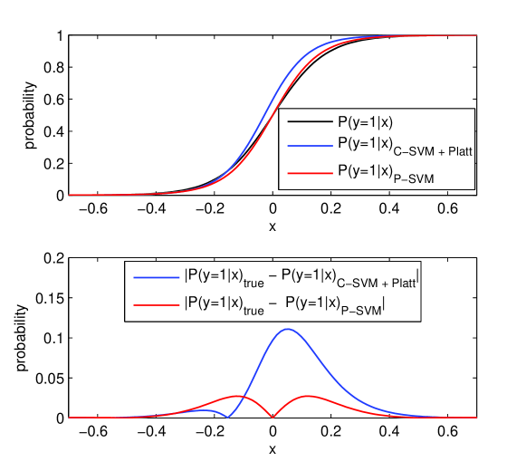
Fig. 1: Probability estimations comparison. Top plot shows the true posterior probabilities with C-SVM and P-SVM estimations overlaying. Lower plot shows the distance between true probabilities and estimations.

5.2 Noise robustness

We generate two 2D datasets, labelled ’+1’ and ’-1’, from normal distributions of variances $\sigma_{-1}^{2}$=$\sigma_{1}^{2}$=0.7 and means $\mu_{-1}$ = (-0.3, -0.5) and $\mu_{1}$=(+0.3, +0.5). As in the previous experiment, we compute class ’1’ membership probability for each point $x^{l}$ of the learning data set. We simulate classification error by artificially adding a centered uniform noise ($\delta$ of amplitude 0.1), to the probabilities, such that for $i=1\dots n$,

$\hat{P}(y_{i}=1|x_{i})=P(y_{i}=1|x_{i})+\delta_{i}$.

We then label learning data following the same scheme as described in (5) and (6). Figure 2 shows the margin location and probabilities estimations using the two methods over a grid of values. Far from learning data points, both probability estimations are less accurate, this being directly linked to the choice of a gaussian kernel. However, P-SVM classification and probability estimations obtained for 1000 test points, are clearly more alike the ground truth (Acc${}_{\textrm{P-SVM}}$ = 99% , KL${}_{\textrm{P-SVM}}$ = 3.6) than C-SVM (Acc${}_{\textrm{C-SVM}}$ = 95%, KL${}_{\textrm{C-SVM}}$ = 95). Contrary to P-SVM which, by combining both classification and regression, predicts good probabilities, C-SVM is sensitive to classification noise and is no more converging to the Bayes rule as seen in [1].

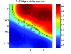
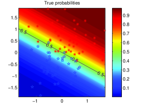
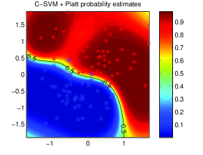
Fig. 2: Probability estimations of C-SVM and P-SVM over a grid using noisy learning data (uniform noise, amplitude 0.1). Noisy learning data are plotted in blue (class ’-1’) and red (class ’1’) stars.

Figure 3 shows the impact of noise amplitude on classifiers performances (values are averaged over 30 random simulations). Even if noise increases, classifications and probability predictions performances of the P-SVM remain significantly higher than those of C-SVM.

Fig. 3: Noise impact on P-SVM and C-SVM classification performances

6 CONCLUSION

This paper has presented a new way to take into account both qualitative and quantitative target data by shrewdly combining both SVM classification and regression loss. Experimental results show that our formulation can perform very well on simulated data for discrimination as well as posterior probability estimation. This approach will soon be applied on clinical data thus allowing to assess its usefulness in computer assisted diagnosis for prostate cancer. Note that this framework initially designed for probabilistic labels can also be generalized to other dataset involving quantitative data as it can be used for instance to estimate a conditional cumulative distribution function.

References

- [1] G. Stempfel and L. Ralaivola, “Learning SVMs from Sloppily Labeled Data,” Artificial Neural Networks–ICANN 2009, pp. 884–893, 2009.
- [2] Bernhard Schölkopf and Alexander J. Smola, Learning with Kernels: Support Vector Machines, Regularization, Optimization, and Beyond (Adaptive Computation and Machine Learning), The MIT Press, 1st edition, December 2001.
- [3] John C. Platt, “Probabilistic outputs for support vector machines and comparisons to regularized likelihood methods,” in Advances in large margin classifiers. 1999, pp. 61–74, MIT Press.
- [4] Peter Sollich, “Probabilistic methods for support vector machines,” in Advances in Neural Information Processing Systems 12. 2000, pp. 349–355, MIT Press.
- [5] S. Rüping, “A Simple Method For Estimating Conditional Probabilities For SVMs,” in LWA 2004, Bickel S. Brefeld U. Drost I. Henze N. Herden O. Minor M. Scheffer T. Stojanovic L. Abecker, A. and S. Weibelza hl, Eds., 2004.
- [6] Y. Grandvalet, J. Mariéthoz, and S. Bengio, “A probabilistic interpretation of SVMs with an application to unbalanced classification,” Advances in Neural Information Processing Systems, vol. 18, pp. 467, 2006.
- [7] S. Rueping, “SVM Classifier Estimation from Group Probabilities,” in ICML 2010.
- [8] S. Canu, Y. Grandvalet, V. Guigue, and A. Rakotomamonjy, “Svm and kernel methods matlab toolbox,” Perception Systèmes et Information, INSA de Rouen, Rouen, France, 2005.