LARGE MARGIN FILTERING FOR SIGNAL Sequence Labeling

Abstract

Signal Sequence Labeling consists in predicting a sequence of labels given an observed sequence of samples. A naive way is to filter the signal in order to reduce the noise and to apply a classification algorithm on the filtered samples. We propose in this paper to jointly learn the filter with the classifier leading to a large margin filtering for classification. This method allows to learn the optimal cutoff frequency and phase of the filter that may be different from zero. Two methods are proposed and tested on a toy dataset and on a real life BCI dataset from BCI Competition III.

Index Terms—  Filtering, SVM ,BCI , Sequence Labeling

1 Introduction

The aim of signal sequence labeling is to assign a label to each sample of a multichannel signal while taking into account the sequentiality of the samples. This problem typically arises in speech signal segmentation or in Brain Computer Interfaces (BCI). Indeed, in real-time BCI applications, each sample of an electro-encephalography signal has to be interpreted as a specific command for a virtual keyboard or a robot hence the need for sample labeling [1, 2].

Many methods and algorithms have already been proposed for signal sequence labeling. For instance, Hidden Markov Models (HMM) [3] are statistical models that are able to learn a joint probability distribution of samples in a sequence and their labels. In some cases, Conditional Random Fields (CRF) [4] have been shown to outperform the HMM approach as they do not suppose the observation are independent. Structural Support Vector Machines (Struct-SVM), which are SVMs that learn a mapping from structured input to structured output, have also been considered for signal segmentation [5]. Signal sequence labeling can also be viewed from a very different perspective by considering a change detection method coupled with a supervised classifier. For instance, a Kernel Change Detection algorithm [6] can be used for detecting abrupt changes in a signal and afterwards a classifier applied for labeling the segmented regions.

In order to preprocess the signal, a filtering is often applied and the resulting filtered samples are used as training examples for learning. Such an approach poses the issue of the filter choice, which is oftenly based on prior knowledge on the information brought by the signals. Moreover, measured signals and extracted features may not be in phase with the labels and a time-lag due to the acquisition process appears in the signals. For example, in the problem of decoding arm movements from brain signals, there exists a natural time shift between these two entries, hence in their works, Pistohl et al. [7] had to select by a validation method a delay in their signal processing method.

In this work, we address the problem of automated tuning of the filtering stage including its time-lag. Indeed, our objective is to adapt the preprocessing filter and all its properties by including its setting into the learning process. Our hypothesis is that by fitting properly the filter to the classification problem at hand, without relying on ad-hoc prior-knowledge, we should be able to considerably improve the sequence labeling performance. So we propose to take into account the temporal neighborhood of the current sample directly into the decision function and the learning process, leading to an automatic setting of the signal filtering.

For this purpose, we first propose a naive approach based on SVMs which consists in considering, instead of a given time sample, a time-window around the sample. This method named as Window-SVM, allows us to learn a spatio-temporal classifier that will adapt itself to the signal time-lag. Then, we introduce another approach denoted as Filter-SVM which dissociates the filter and the classifier. This novel method jointly learns a SVM classifier and FIR filters coefficients. By doing so, we can interpret our filter as a large-margin filter for the problem at hand. These two methods are tested on a toy dataset and on a real life BCI signal sequence labeling problem from BCI Competition III [1].

2 Large margin filter

2.1 Problem definition

Our concern is a signal sequence labeling problem : we want to obtain a sequence of labels from a multichannel time-sample of a signal or from multi-channel features extracted from that signal. We suppose that the training samples are gathered in a matrix $X\in\mathbb{R}^{N\times d}$ containing $d$ channels and $N$ samples. $X_{i,j}$ is the value of channel $j$ for the $i^{th}$ sample. The vector $\mathbf{y}\in\{-1,1\}^{N}$ contains the class of each sample.

In order to reduce noise in the samples or variability in the features, an usual approach is to filter $X$ before the classifier learning stage. In literature, all channels are usually filtered with the same filter (Savisky-Golay for instance in [7]) although there is no reason for a single filter to be optimal for all channels. Let us define the filters applied to $X$ by the matrix $F\in\mathbb{R}^{f\times d}$. Each column of $F$ is a filter for the corresponding channel in $X$ and $f$ is the size of the FIR filters.

We define the filtered data matrix $\widetilde{X}$ by:

$$\widetilde{X}_{i,j}=\sum_{m=1}^{f}~{}F_{m,j}~{}X_{i+1-m+n_{0},j}$$ (1)

where the sum is a unidimensional convolution of each channel by the filter in the appropriate column of $F$. $n_{0}$ is the delay of the filter, for instance $n_{0}=0$ corresponds to a causal filter and $n_{0}=f/2$ corresponds to a filter centered on the current sample.

2.2 Windowed-SVM (W-SVM)

As highlighted by Equation (1), a filtering stage essentially consists in taking into account for a given time $i$, instead of the sample $X_{i,\cdot}$, a linear combination of its temporal neighborhood. However, instead of introducing a filter $F$, it is possible to consider for classification a temporal window around the current sample. Such an approach would lead to this decision function for the $i^{th}$ sample of $X$:

$$f_{W}(i,X)=\sum_{m=1}^{f}\sum_{j=1}^{d}W_{m,j}X_{i+1-m+n_{0},j}+w_{0}$$ (2)

where $W\in\mathbb{R}^{f\times d}$ and $w_{0}\in\mathbb{R}$ are the classification parameters and $f$ is the size of the time-window. Note that $W$ plays the role of the filter and the weights of a linear classifier. In a large-margin framework, $W$ and $w_{0}$ may be learned by minimizing this functional:

$$J_{WSVM}(W)=\frac{1}{2}||W||_{F}^{2}+\frac{C}{2}\sum_{i=1}^{N}H(\mathbf{y},X,f_{W},i)^{2}\\$$ (3)

where ${||W||}_{F}^{2}=\sum_{i,j}W_{i,j}^{2}$ is the squared Frobenius norm of $W$, $C$ is a regularization term to be tuned and $H(\mathbf{y},X,f,i)=\max(0,1-\mathbf{y}_{i}f(i,X))$ is the SVM hinge loss. By vectorizing appropriately $X$ and $W$, problem (3) may be transformed into a linear SVM. Hence, we can take advantage of many linear SVM solvers existing in the literature such as the one proposed by Chapelle [8]. By using that solver, Window-SVM complexity is about $\mathcal{O}(N.(f.d)^{2})$ which scales quadratically with the filter dimension.

The matrix $W$ weights the importance of each sample value $X_{i,j}$ into the decision function. Hence, channels may have different weights and time-lag. Indeed, $W$ will automatically adapt to a phase difference between the sample labels and the channel signals. However, in this method since space and time are treated independently, $W$ does not take into account the multi-channel structure and the sequentiality of the samples. Since the samples of a given channel are known to be time-dependent due to the underlying physical process, it seems preferable to process them with a filter and to classify the filtered samples. So we propose in the sequel another method that jointly learns the time-filtering and a linear classifier on the filtered sample defined by Eq. (1).

2.3 Large margin filtering (Filter-SVM)

We propose to find the filter $F$ that maximizes the margin of the linear classifier for the filtered samples. In this case, the decision function is:

$$f_{F}(i,X)=\sum_{m=1}^{f}\sum_{j=1}^{d}\mathbf{w}_{j}F_{m,j}X_{i+1-m+n_{0},j}+w_{0}$$ (4)

where $\mathbf{w}$ and $w_{0}$ are the parameters of the linear SVM classifier corresponding to a weighting of the channels. By dissociating the filter and the decision function weights, we expect that some useless channels (non-informative or too noisy) for the decision function get small weights. Indeed, due to the double weighting $\mathbf{w}_{j}$ and $F_{.,j}$, and the specific channel weighting role played by $\mathbf{w}_{j}$, this approach, as shown in the experimental section is able to perform channel selection.

The decision function given in Equation (4) can be obtained by minimizing:

$$J_{FSVM}=\frac{1}{2}||\mathbf{w}||^{2}+\frac{C}{2}\sum_{i=1}^{n}H(\mathbf{y},X,f_{F},i)^{2}+\frac{\lambda}{2}{||F||}^{2}_{F}$$ (5)

w.r.t. $(F,\mathbf{w},w_{0})$ where ${||F||}_{F}$ is the Frobenius norm, and $\lambda$ is a regularization term to be tuned. Note that without the regularization term ${||F||}^{2}_{F}$, the problem is ill-posed. Indeed, in such a case, one can always decrease $||\mathbf{w}||^{2}$ while keeping the empirical hinge loss constant by multiplying $w$ by $\alpha<1$ and $F$ by $\frac{1}{\alpha}$ .

The cost defined in Equation (5) is differentiable and provably non-convex when jointly optimized with respect to all parameters. However, $J_{FSVM}$ is differentiable and convex with respect to $\mathbf{w}$ and $w_{0}$ when $F$ is fixed as it corresponds to a linear SVM with squared hinge loss. Hence, for a given value of $F$, we can define

$$J(F)=\min_{\mathbf{w},w_{0}}\frac{1}{2}||\mathbf{w}||^{2}+\frac{C}{2}\sum_{i=1}^{n}H(\mathbf{y},X,f_{F},i)^{2}$$

which according to Bonnans et al. [9] is differentiable. Then if $\mathbf{w}^{*}\text{ and }w_{0}^{*}$ are the optimal values for a given $F^{*}$, the gradient of the second term of $J(\cdot)$ with respect to $F$ at the point $F^{*}$ is:

$$\nabla_{F_{m,j}}J(F^{*})=-\sum_{i=1}^{N}\mathbf{y}_{i}(\mathbf{w}^{*}_{j}X_{i-m+1+n_{0},j})\times H(\mathbf{y},X,f_{F^{*}},i)$$

Now, since $J(F)$ is differentiable and since its value can be easily computed by a linear SVM, we choose for learning the decision function to minimize $J(F)+\frac{\lambda}{2}\|F\|_{F}^{2}$ with respects to $F$ instead of minimizing problem (5). Note that due to the objective function non-convexity in problem (5), these two minimization problems are not strictly equivalent, but our approach has the advantage of taking into account the intrinsic large-margin structure of the problem.

Algorithm 1 Filter-SVM solver

  Set $F_{l,k}=1/f$ for $k=1\cdots d$ and $l=1\cdots f$

  repeat

     $D_{F}\leftarrow$ gradient of $J_{FSVM}$ with respect to $F$

     $(F,w^{*},w_{0}^{*})\leftarrow$ Line-Search along $D_{F}$

  until  Stopping criterion is reached

For solving the optimization problem, we propose a gradient descent algorithm along $F$ with a line search method for finding the optimal step. The method is detailed in algorithm 1. Note that at each computation of $J(F)$ in the line search, the optimal $\mathbf{w}^{*}\text{ and }w_{0}^{*}$ are found by solving a linear SVM. The iterations in the algorithm may be stopped by two stopping criteria: a threshold on the relative variation of $J(F)$ or a threshold on variations of $F$ norm.

Due to the non-convexity of the objective function, it is difficult to provide an exact evaluation of the solution complexity. However, we know that the gradient computation has order of $\mathcal{O}(N.f.d)$ and that when $J(F)$ is computed at each step of the line search, a $\mathcal{O}(N.d^{2})$ linear SVM is solved and a $\mathcal{O}(N.f.d)$ filtering is applied.

3 Results

3.1 Toy Example

We use a toy example that consists of $nbtot$ channels, only $nbrel$ of them being discriminative. Discriminative channels have a switching mean $\{-1,1\}$ controlled by the label and corrupted by a gaussian noise of deviation $\sigma$. The length of the regions with constant label follows a uniform distribution law between $[30,40]$ samples and different time-lags are applied to the channels. We selected $f=21$ and $n_{0}=11$ corresponding to a good average filtering centered on the current sample.

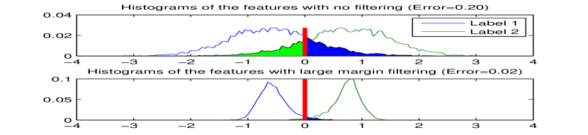
Fig. 1: Histograms of both labels with and without filtering (vertical axis are different) for a 1 channel signal with $\sigma=1$

Figure 1 shows how the samples are transformed thanks to the filter $F$ for a unidimensional signal. In this case, the mean test error due to the noise is 16% for the unfiltered signal, while only 2% for the optimally filtered signal.

Window-SVM and Filter-SVM are compared to SVM without filtering, SVM with an average filter of size $f$ (Avg-SVM) and HMM with a Viterbi decoding. The regularization parameters are selected by a validation method. The size of the signals is of $1000$ samples for the learning and the validation sets and of $5000$ samples for the test set. All the processes are run ten times, the test error is the the average over the runs.

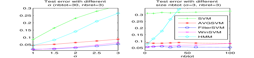
Fig. 2: Test error for different $\sigma$ values ($nbtot=~{}30$, $nbrel=~{}3$, on the left) and for different number of channels $nbtot$ ($\sigma=~{}3$, $nbrel=~{}3$, on the right)

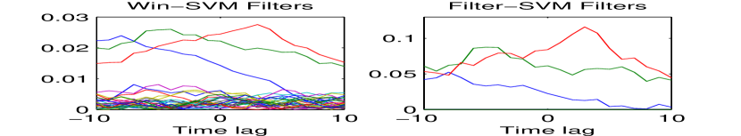
Fig. 3: Coefficients of $W$ (left) and coefficients $F$ weighted by $w$ (right) for $nbrel=3$, $nbtot=30$, $\sigma=3$

The methods are compared for different $\sigma$ values with ($nbtot=30$, $nbrel=3$). The test error is plotted on the left of Figure 2. We can see that only Avg-SVM, Window-SVM and Filter-SVM adapt to time-lags between the channels and the labels. Both Window-SVM and Filter-SVM outperform the other methods, even if for a heavy noise, the last one seems to be slightly better. Then we test our methods for a varying number of channels in order to see how dimension is handled ($nbrel=3$, $\sigma=3$). Figure 2 (right) shows the interest of Filter-SVM over Window-SVM in hight dimension as we can see that the last one tends to lose his efficiency, and even to be similar to Avg-SVM. This comes from the fact that Filter-SVM can more efficiently perform a channel selection thanks to the weighting of $\mathbf{w}$. Figure 3 shows the filters returned by both methods. We observe that only the coefficients of the relevant signals are important and that the other signals tend to be eliminated by small weights for Filter-SVM, explaining the better results in high dimension.

3.2 BCI Dataset

We test our method on the BCI Dataset from BCI Competition III [1]. The problem is to obtain a sequence of labels out of brain activity signals for 3 human subjects. The data consists in 96 channels containing PSD features (3 training sessions, 1 test session, $N\approx{3000}$ per session) and the problem has 3 labels (left arm, right arm or feet).

We use Filter-SVM that showed better result in hight dimension for the toy example. The multi-class aspect of the problem is handled by using a One-Against-All strategy. The regularization parameters are tuned using a grid search validation method on the third training set. We compare our method to the best BCI competition results (using only 8 samples) and to the SVM without filtering. Test error for different filter size $f$ and delay $n_{0}$ may be seen on Table 1.

Method	Sub 1	Sub 2	Sub3	Avg
BCI Comp.	0.2040	0.2969	0.4398	0.3135
SVM	0.2877	0.4283	0.5209	0.4123
Filter-SVM
$f=8,n_{0}=0$	0.2337	0.3589	0.4937	0.3621
$f=20,n_{0}=0$	0.2021	0.2693	0.4381	0.3032
$f=50,n_{0}=0$	0.1321	0.2382	0.4395	0.2699
Avg-SVM
$f=100,n_{0}=50$	0.1544	0.2235	0.3870	0.2550
Filter-SVM
$f=100,n_{0}=50$	0.0537	0.1659	0.3859	0.2018

Table 1: Test Error for BCI Dataset

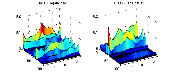
Fig. 4: $F$ filters (subject 1) for label 1 against all (left) and label 2 against all (right).

Results show that one can improve drastically the result by using longer filtering with causal filters ($n_{0}=0$). Note that Filter-SVM outperform Avg-SVM with a centered filter.

Another advantage of this method is that one can visualize a discriminative space-time map (channel selection, shape of the filter and delays). We show for instance in Figure 4 the discriminative filters $F$ obtained for subject 1, and we can see that the filtering is extremely different depending on the task.

The Matlab code corresponding to these results will be provided on our website for reproducibility.

4 Conclusions

We have proposed two methods for automatically learning a spatio-temporal filter used for multi-channel signal classification. Both methods have been tested on a toy example and on a real life dataset from BCI Competition III.

Empirical results clearly show the benefits of adapting the signal filter to the large-margin classification problem despite the non-convexity of the criterion.

In future work, we plan to extend our approach to non-linear case, we believe that a differentiable kernel can be used instead of inner products at the cost of solving the SVM in the dual space. Another perspective would be to adapt our methods to the multi-task situation, where one wants to jointly learn one matrix $F$ and several classifiers (one per task).

References

- [1] B. Blankertz et al., “The BCI competition 2003: progress and perspectives in detection and discrimination of EEG single trials,” IEEE Transactions on Biomedical Engineering, vol. 51, no. 6, pp. 1044–1051, 2004.
- [2] J. del R Millán, “On the need for on-line learning in brain-computer interfaces,” in Proc. Int. Joint Conf. on Neural Networks, 2004.
- [3] O. Cappé, E. Moulines, and T. Rydèn, Inference in Hidden Markov Models, Springer, 2005.
- [4] J. Lafferty, A.McCallum, and F. Pereira, “Conditional random fields: Probabilistic models for segmenting and labeling sequence data,” in Proc. 18th International Conf. on Machine Learning, 2001, pp. 282–289.
- [5] I. Tsochantaridis, T. Joachims, T. Hofmann, and Y. Altun, “Large margin methods for structured and interdependent output variables,” in Journal Of Machine Learning Research. 2005, vol. 6, pp. 1453–1484, MIT Press.
- [6] F. Desobry, M. Davy, and C. Doncarli, “An online kernel change detection algorithm,” IEEE Transactions on Signal Processing, vol. 53, pp. 2961–2974, 2005.
- [7] T. Pistohl, T. Ball, A. Schulze-Bonhage, A. Aertsen, and C. Mehring, “Prediction of arm movement trajectories from ecog-recordings in humans,” Journal of Neuroscience Methods, vol. 167, no. 1, pp. 105–114, Jan. 2008.
- [8] O. Chapelle, “Training a support vector machine in the primal,” Neural Comput., vol. 19, no. 5, pp. 1155–1178, 2007.
- [9] J.F. Bonnans and A. Shapiro, “Optimization problems with pertubation : A guided tour,” SIAM Review, vol. 40, no. 2, pp. 202–227, 1998.