Controlling Excitations Inversion of a Cooper Pair Box Interacting with a Nanomechanical Resonator

Abstract

We investigate the action of time dependent detunings upon the excitation inversion of a Cooper pair box interacting with a nanomechanical resonator. The method employs the Jaynes-Cummings model with damping, assuming different decay rates of the Cooper pair box and various fixed and t-dependent detunings. It is shown that while the presence of damping plus constant detunings destroy the collapse/revival effects, convenient choices of time dependent detunings allow one to reconstruct such events in a perfect way. It is also shown that the mean excitation of the nanomechanical resonator is more robust against damping of the Cooper pair box for convenient values of t-dependent detunings.

1 Introduction

A popular and exactly soluble model in quantum optics is the Jaynes-Cumming model (JCM). It describes the interaction of a two-level atom with a single-mode of the electromagnetic field [1, 2, 3, 4, 5, 6, 7]. Over the last two decades various extensions of the ordinary JCM have been used in various directions, e.g., as adapted to: (i) the study of interaction of a three-level atom with a two-mode squeezed vacuum [8]; (ii) the study of atom-field interaction in the presence of a cavity damping [9]; (iii) the same as in (i), including an additional (nonlinear) Kerr medium [10]; (iv) the two-level atoms inside a cavity acted upon by an external field control [11]; (v) study of the nonlinear dynamical evolution of a driven two-photon Jaynes-Cummings model [13]; (vi) the study of a generalized Jaynes-Cummings models, including dissipation [14, 15, 16] and multiphoton interactions [17, 18]; etc. In all these cases, with interest either on the field or on atomic properties, the theoretical approach traditionally assumes the atom-field coupling as a constant parameter. Comparatively, the number of works in the literature is very small when one considers such coupling and the atomic frequency as time dependent parameters [19, 20, 21, 22, 23, 12], including time dependent amplitudes [24]. However, this scenario is also relevant;  for example, the state of two qubits (qubits stand for quantum bits) with a desired degree of entanglement can be generated via a time dependent atom-field coupling [25]. Actually, such coupling can modify the dynamical properties of the atom and the field, with transitions that involve a large number of photons [26]. In general, these studies are simplified by neglecting the atomic decay from an excited level. Theoretical treatments taking into account this complication of the real world may employ a modified JCM. In these case, as expected, the state describing the system decoheres, since the presence of dissipation destroys the state of a system as time flows.

In the present work we extend what we have learned from the JCM applied to the atom-field interaction to investigate a more advantageous system, from the experimental viewpoint (faster response, better controllability, and useful scalability for quantum computation [27] ) by considering a nanomechanical resonator (NR) interacting with a Cooper pair box (CPB) [17, 15, 28]. Such nanodevice has been explored extensively in the literature, e.g., to investigate: (i) quantum nondemolition measurements [29, 30], (ii) decoherence of nonclassical states, as Fock states and superposition states describing mesoscopic systems [31, 32], etc. The fast advance in the technique of fabrication in nanotechnology has implied great interest in the study of the NR system in view of its potential applications, as a sensor - to be used in biology, astronomy, quantum computation, and in quantum information [33, 34, 35], to implement the quantum qubit [36] and in the production of nonclassical states, as Fock state [37, 38], Schrödinger’s cat state [39], squeezed states [40], clusters states [41], etc. In particular, when accompanied by superconducting charge qubits, the NR has been used to prepare entangled states [42]. Zhou et al.[40] have proposed a scheme to prepare squeezed states using a NR coupled to a CPB qubit; in this proposal the NR-CPB coupling is under an external control while the connection between these two subsystems plays an important role in quantum computation. Such a control is achieved via convenient change of the system parameters, which can set “on” and “off” the interaction between the NR and the CPB, on demand.

In this report we will investigate the CPB excitation inversion, its control, and the average photon number in the NR. We will consider dissipation in the CPB due to a decay rate from excited to ground states. We will also verify in which way the time dependence of the CPB-NR coupling modifies these two properties. To this end we must solve the time evolution of the whole CPB-NR system, via the approach presented in the following Section.

2 Model Hamiltonian for the CPB-NR system

A Josephson charge qubit system has been used to couple with a NR. Here we study a modified model where a CPB is coupled to a NR, as shown in Fig. 1 below. The scheme is inspired by the works of Jie-Qiao Liao et al. [36] and Zhou et al. [40] where we have substituted each Josephson junction by two of them. This creates a new configuration that includes a third loop. A superconducting CPB charge qubit is adjusted via a voltage $V_{1}$ at the system input and a capacitance $C_{g}$. We want that the scheme attains an efficient tunneling effect for the Josephson energy. In Fig. 1 we observe three loops: one great loop between two small ones. This makes it easier controlling the external parameters of the system since the control mechanism includes the input voltage $V_{1}$ plus three external fluxes $\Phi_{L},$ $\Phi_{r}$ and $\Phi_{e}(t)$. In this way one can induce small neighboring loops. The great loop contains a NR which is modeled as a harmonic oscillator with a high-Q mode of frequency $\Omega$ and its effective area in the center of the apparatus changes as the NR oscillates, which creates an external flux $\Phi_{e}(t)$ that provides the CPB-NR coupling.

In pursuing the quantum behavior of a macro scale object the nano scale mechanical resonator plays an important role. At sufficiently low temperature the zero-point fluctuation of the NR will be comparable to its thermal Brownian motion. The detection of zero-point fluctuations of the NR can give a direct test of Heisenberg’s uncertainty principle. With a sensitivity up to 10 times the amplitude of the zero-point fluctuation, LaHaye et al [43] have experimentally detected the vibrations of a 20 MHz mechanical beam of tens of micrometres size. For a 20MHz mechanical resonator its temperature must be cooled below 1mK to suppress the thermal fluctuation. For a GHz mechanical resonator a temperature of 50mK is sufficient to effectively freeze out its thermal fluctuation and let it enter the quantum regime. This temperature is already attainable in dilution refrigerators.

Figure 1: Model for the CPB-NMR coupling.

In this work we will assume the four Josephson junctions being identical, with the same Josephson energy $E_{J}^{0}$, the same being assumed for the external fluxes $\Phi_{L}$ and $\Phi_{r}$, i.e., with same magnitude but opposite sign: $\Phi_{L}=-\Phi_{r}=\Phi_{x}$. This interaction actually couples the two subsystems. Together with the free Hamiltonian of flux qubit and NR, the Hamiltonian of the whole system reads

$$\hat{H}=\Omega\hat{a}^{\dagger}\hat{a}+4E_{c}\left(N_{g}-\frac{1}{2}\right)\hat{\sigma}_{z}-4E_{J}^{0}\cos\left(\frac{\pi\Phi_{x}}{\Phi_{0}}\right)\cos\left(\frac{\pi\Phi_{e}}{\Phi_{0}}\right)\hat{\sigma}_{x},$$ (1)

where $\hat{a}^{\dagger}(\hat{a})$ is the creation (annihilation) operator for the NR excitation, with frequency $\Omega$  and mass $m$; $E_{J}^{0}$ and $E_{c}$ are respectively the energy of each Josephson junction and the charge energy of a single electron; $C_{g}$ and $C_{J}^{0}$ are the input capacitance and the capacitance of each Josephson tunnel, respectively. $\Phi_{0}=h/2e$ is the quantum flux and $N_{g}=C_{g}V_{1}/2e$ is the charge number in the input with the input voltage $V_{1}$. We have used the Pauli matrices to describe our system operators, where the states $\left|0\right\rangle$ and $\left|1\right\rangle$ represent the number of extra Cooper pairs in the superconducting island. We have: $\hat{\sigma}_{z}=\left|0\right\rangle\left\langle 0\right|-\left|1\right\rangle\left\langle 1\right|$, $\hat{\sigma}_{x}=\left|0\right\rangle\left\langle 1\right|-\left|1\right\rangle\left\langle 0\right|$ and $E_{C}=e^{2}/\left(C_{g}+4C_{J}^{0}\right).$

The magnetic flux can be written as the sum of two terms,

$$\Phi_{e}=\Phi_{1}+B\ell\hat{x},$$ (2)

where the first term $\Phi_{1}$ is the induced flux, corresponding to the equilibrium position of the NR and the second term describes the contribution due to the vibration of the NR; $B$ represents the magnetic field created in the loop. We have assumed the displacement $\hat{x}$ described as $\hat{x}=x_{0}(\hat{a}^{\dagger}+\hat{a})$, where $x_{0}=\sqrt{m\Omega/2}$ is the amplitude of the oscillation. Substituting the Eq.(2) in Eq.(1) and controlling the flux $\Phi_{1}$ we can adjust $\cos\left(\frac{\pi\Phi_{1}}{\Phi_{0}}\right)=0$, and making the approximation $\pi B\ell x/\Phi_{0}<<1$ the above Hamiltonian results as (in rotating wave approximation),

$$\hat{H}=\Omega\hat{a}^{\dagger}\hat{a}+\frac{1}{2}\omega_{0}\hat{\sigma}_{z}+\lambda_{0}(\hat{\sigma}_{+}\hat{a}+\hat{a}^{\dagger}\hat{\sigma}_{-}),$$ (3)

where the constant coupling $\lambda_{0}=-4E_{J}^{0}\cos\left(\frac{\pi\Phi_{x}}{\Phi_{0}}\right)\left(\frac{\pi B\ell x_{0}}{\Phi_{0}}\right)$ and the effective energy $\omega_{0}=8E_{c}\left(N_{g}-\frac{1}{2}\right).$ An important advantage of this coupling mechanism is its easy and convenient controllability.

Next, we will extend the previous approach to a more general scenario by substituting $\Omega\rightarrow\omega(t)=\Omega+f\left(t\right)$ and $\lambda_{0}\rightarrow\lambda(t)=\lambda_{0}\left[1+f\left(t\right)/\Omega\right]$ [26, 44, 45]; in addition we assume the presence of a constant decay rate $\gamma$ in the CPB; $\omega_{0}$ is the transition frequency of the CPB and $\lambda_{0}$ stands for the CPB-NR coupling. $\hat{\sigma}_{\pm}$ and $\hat{\sigma}_{z}$ are the CPB transition and excitation inversion operators, respectively; they act on the Hilbert space of atomic states and satisfy the commutation relations $\left[\hat{\sigma}_{+},\hat{\sigma}_{-}\right]=\hat{\sigma}_{z}$ and $\left[\hat{\sigma}_{z},\hat{\sigma}_{\pm}\right]=\pm\hat{\sigma}_{\pm}$. As well known, the coupling parameter $\lambda(t)$ is proportional to $\sqrt{\omega(t)/V\left(t\right)}$, where the time dependent quantization volume $V\left(t\right)$ takes the form $V\left(t\right)=V_{0}/\left[1+f\left(t\right)/\Omega\right]$ [46, 22, 45]. Accordingly, we obtain the new (non hermitian) Hamiltonian

$$\hat{H}=\omega(t)\hat{a}^{\dagger}\hat{a}+\frac{1}{2}\omega_{0}\hat{\sigma}_{z}+\lambda(t)(\hat{\sigma}_{+}\hat{a}+\hat{a}^{\dagger}\hat{\sigma}_{-})-i\frac{\gamma}{2}\left|1\right\rangle\left\langle 1\right|.$$ (4)

It is worth remembering that non Hermitian Hamiltonians (NHH) are largely used in the literature. To give some few examples we mention: Ref. [47], where the authors use a NHH and an algorithm to generalize the conventional theory; Ref. [48], using a NHH to get information about entrance and exit channels; Ref. [49], using non Hermitian techniques to study canonical transformations in quantum mechanics; Ref. [50], solving quantum master equations in terms of NHH; Ref. [51], using a new approach for NHH to study the spectral density of weak H-bonds involving damping; Ref. [52], studying NHH with real eigenvalues; Ref. [53], using a canonical formulation to study dissipative mechanics exhibing complex eigenvalues; Ref. [54], studying NHH in non commutative space, and more recently: Ref. [55], studying the optical realization of relativistic NHH; Ref. [22], studying the evolution of entropy of atom-field interaction; Ref. [21], using a damping JC-Model to study entanglement between two atoms, each of them lying inside different cavities

3 Solving the CPB-NR system

The state that describes this time dependent system can be written in the form

$$\left|\Psi\left(t\right)\right\rangle=\sum\nolimits_{n=0}^{\infty}(C_{0,n}\left(t\right)\left|0,n\right\rangle+C_{1,n}\left(t\right)\left|1,n\right\rangle),$$ (5)

where $\left|0,n\right\rangle$ $\left(\left|1,n\right\rangle\right)$ represents the CPB in its excited state $\left|1\right\rangle$ (ground state $\left|0\right\rangle$). Taking the CPB initially prepared in its excited state $\left|1\right\rangle$ and the NR in a coherent states $\left|\alpha\right\rangle$, and expanding coherent state component in the Fock’s basis, i.e., $\left|\alpha\right\rangle=exp(-|\alpha|^{2}/2)\sum_{n=o}^{\infty}(\alpha^{n}/\sqrt{n!})|n\rangle$, we have $\left|\alpha\right\rangle=\sum\nolimits_{n=0}^{\infty}F_{n}\left|n\right\rangle$. Assuming the NR and CPB decoupled at $t=0$ and the initial conditions $C_{0,n}\left(0\right)=0$ and $\sum\nolimits_{n=0}^{\infty}\left|C_{1,n}\left(0\right)\right|^{2}=1$ we may write the Eq. (5) as $\left|\Psi\left(0\right)\right\rangle=\sum\nolimits_{n=0}^{\infty}F_{n}\left|1,n\right\rangle.$

The time dependent Schrödinger equation for this system is

$$i\frac{d\left|\Psi\left(t\right)\right\rangle}{dt}=\hat{H}\left|\Psi\left(t\right)\right\rangle,$$ (6)

with the Hamiltonian $\hat{H}$ given in Eq. (4). Substituting Eq.(4) in Eq.(6) we get the (coupled) equations of motion for the probabilitity amplitudes $C_{1,n}(t)$ and $C_{0,n+1}(t)$:

$$\frac{\partial C_{1,n}(t)}{\partial t} = -in\omega(t)C_{1,n}(t)-\frac{i}{2}\omega_{0}C_{1,n}(t)-i\lambda(t)\sqrt{n+1}C_{0,n+1}(t)-\frac{\gamma}{2}C_{1,n}(t),\phantom{aaaaaa}$$ (7)

$$\frac{\partial C_{0,n+1}(t)}{\partial t} = -i(n+1)\omega(t)C_{0,n+1}(t)+\frac{i}{2}\omega_{0}C_{0,n+1}(t)-i\lambda(t)\sqrt{n+1}C_{1,n}(t).$$ (8)

The numerical solutions of the coefficients $C_{1,n}(t)$, $C_{0,n+1}(t)$ furnish the quantum dynamical properties of the system, including the CPB-NR entanglement.

As well known, in the presence of decay rate $\gamma$ in the CPB the state of the whole CPB-NR system becomes mixed. In this case its description requires the use of the density operator $\hat{\rho}_{CN}$, which describes the entire system. To obtain the reduced  density matrix describing the CPB (NR) subsystem we must trace over variables of the NR (CPB) subsystem. For example, $\hat{\rho}_{NR}=Tr_{CPB}(\hat{\rho}_{CN})$:

$$\hat{\rho}_{NR}=\sum\nolimits_{n,n^{\prime}=o}^{\infty}\left[C_{1,n}(t)C_{1,n^{\prime}}^{\ast}(t)+C_{0,n}(t)C_{0,n^{\prime}}^{\ast}(t)\right]\left|n\right\rangle\left\langle n\prime\right|.$$ (9)

4 Excitation Inversion of the CPB

The CPB excitation inversion, here denoted as $I(t)_{CPB}$, is an important observable of two level systems. It is defined as the difference of probabilities of finding the system in the excited and ground state, as follows

$$I(t)_{{CPB}}=\sum\nolimits_{n=0}^{\infty}\left[\left|C_{1,n}(t)\right|^{2}-\left|C_{0,n+1}(t)\right|^{2}\right].$$ (10)

The Eq. (10) allows one to look at the time evolution of the CPB excitation inversion. First, we assume the resonant case $(f(t)=0)$ for different values of the decay rate $\gamma$, with $\alpha=5$ and $\Omega=\omega_{0}=2000\lambda_{0}$ and assuming the NR initially in a coherent state with the average number of excitations $\left\langle n\right\rangle=25$ as shown in Fig. 2. With the exceptions of amplitudes, the plots (a), (b) and (c) of Fig. 2 show identical for collapse-revival effects: the higher the decay rate the lower is the amplitude of oscillation. In presence of detuning, where $f(t)=\Delta=const$, where $\Delta\ll\omega_{0}$, $\Omega$, we see that the excitation inversion in Fig. 3(a) occurs within the interval $30<\lambda_{0}t<50$, whereas in Fig. 3(b) it occurs in the range $60<\lambda_{0}t<75$ and in Fig. 3(c) the excitation inversion goes to zero rapidly. Considering the case of variable detuning, $f(t)=\eta\sin(\omega\prime t)$, we see in the plots (a), (b) and (c) of Fig. 4 that the excitation inversion occurs frequently in Fig. 4(a) and desapears when the parameter $\eta$ increases, as shown in the plots (b) and (c). Now, even considering the worst results obtained in the off-resonant cases, with detuning $\Delta=\eta=60\lambda_{0}$, as shown in Fig. 3(c) and Fig. 4(c) we see that we can recover the collapse-revival effects via the increase of the parameter $\omega\prime,$ as shown in the plots (a), (b) and (c) of Fig. 5. So, the parameter $\omega\prime$ plays a fundamental role in the control of collapse and revival effect.

Fig. 6 shows plots of the mean value of the NR excitations in the presence of CPB decay rate for various values of amplitude of oscillations (parameter $\eta$). Plots (d) and (h) are for the resonant case: in (d) the decay rate is greater than in (h). Plots (a), (b), and (c) are for constant decay rates, with (time independent) detuning that increases from (c) $\rightarrow$ (b) $\rightarrow$ (a). Finally, plots (e), (f) and (g) are for time dependent detuning, with the parameter $\eta$ increasing from (e) $\rightarrow$ (f) $\rightarrow$ (g).  We note that the three plots for time dependent detunings (e), (f) and (g) are better than those for constant detunings (a), (b) and (c): despite all plots are concerned with the same decay rate, the first group is more robust against decay. For example, comparing the plots (a) and (g): although in (a) the fixed detuning is $\Delta=60\lambda_{0}$ and in (g) maximum detuning is $\Delta_{\max}=\eta=60\lambda_{0}$ we see that in the last case the average value of the NR decays more slowly. One observes in the plot (c) of Fig. 5 that the interval $\lambda_{0}t$, where the presence of the time dependent detuning recovers the collapse-revival effect, coincides with that in the plot (g) of Fig. 6 where the mean value of excitation is around 5 times greater than in the case of constant detuning (plot (a) of same figure).

Figure 2: Time evolution of the Excitation Inversion in the CPB with $\left\langle n\right\rangle=25$, $\Omega=\omega_{0}=2000\lambda_{0}$, for $f(t)=0$ (resonance) and different values of decay rates $\gamma$: (a) $\gamma=0.01\lambda_{0}$, (b) $\gamma=0.05\lambda_{0}$ and (c) $\gamma=0.5\lambda_{0}$.

Figure 3: Same as in Fig. 2 for $\gamma=0.05\lambda_{0}$ and different values of detunings $($cf. $f(t)=\Delta=const.)$: (a) $\Delta=10\lambda_{0}$ , (b) $\Delta=20\lambda_{0}$, (c) $\Delta=60\lambda_{0}$.

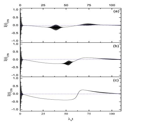
Figure 4: Same as in Fig. 2 for $\gamma=0.05\lambda_{0}$ and different time-dependent detunings (cf. $f(t)=\eta\sin(\omega\prime t)$): (a) $\eta=10\lambda_{0}$ and $\omega\prime=0.05\lambda_{0}$, (b) $\eta=20\lambda_{0}$ and $\omega\prime=0.05\lambda_{0},$ (c) $\eta=60\lambda_{0}$ and $\omega\prime=0.05\lambda_{0}.$

Figure 5: Same as in Fig. 2 for $\gamma=0.05\lambda_{0}$ and different time-dependent detunings (cf. $f(t)=\eta\sin(\omega\prime t)$): (a) $\eta=60\lambda_{0}$ and $\omega\prime=20\lambda_{0}$, (b) $\eta=60\lambda_{0}$ and $\omega\prime=40\lambda_{0},$ (c) $\eta=60\lambda_{0}$ and $\omega\prime=58\lambda_{0}$.

Figure 6: Average number of excitations of the NR, versus time, for $\left\langle n(0)\right\rangle=25$, $\Omega=\omega_{0}=2000\lambda_{0}$, for the following cases: (a) off-resonance $\gamma=0.05\lambda_{0}$, $\Delta=60\lambda_{0},$ (b) off-resonance $\gamma=0.05\lambda_{0}$, $\Delta=20\lambda_{0},$ (c) off-resonance $\gamma=0.05\lambda_{0}$, $\Delta=10\lambda_{0},$  (d) on resonance $\gamma=0.5\lambda_{0},$ (e) off-resonance $\gamma=0.05\lambda_{0},$ $\eta=10\lambda_{0}$ and $\omega\prime=0.05\lambda_{0},$ (f) off-resonance $\gamma=0.05\lambda_{0},$ $\eta=20\lambda_{0}$ and $\omega\prime=0.05\lambda_{0},$(g) off-resonance $\gamma=0.05\lambda_{0},$ $\eta=60\lambda_{0}$ and $\omega\prime=0.05\lambda_{0},$ (h) on resonance $\gamma=0.05\lambda_{0}$.

5 Conclusion

We have considered a Hamiltonian model that describes a CPB-NR interacting system to study the CPB excitation inversion, $I(t)_{{CPB}},$ and the average excitation number of the NR, $\left\langle n(t)\right\rangle_{NR}$. We have also considered the off-resonant case, with various values of the detuning parameter $f\$($f=0;f=\Delta;$ and $f=\eta\sin(\omega\prime t)$) and in the presence of CPB decay (about 10 times greater than the (neglected) NR decay). These properties are characteristics of the entangled state that describes this coupled system for various values of the parameters involved. We have assumed the CPB initially in its excited state and the NR initially in a coherent state (see preparation in [17]). So, the following three scenarios were treated: (i) both subsystems in resonance (detuning $f=0$); (ii) off-resonance, with a constant detuning $(f=\Delta\neq 0)$, and (iii) with a time dependent detuning $(f(t)=\eta\sin(\omega\prime t))$. The results were discussed in the previous Section: in resume, concerning the CPB excitation inversion, an interesting result emerged: although the presence of a constant detuning destroys the collapse and revivals of the excitation inversion, these effects are restituted by the action of convenient time dependent detunings - even in the presence of damping in the CPB; concerning the NR average excitation number, another interesting result appeared: convenient choices of the time dependent detuning $f(t)$ makes the NR subsystem more robust against the decay affecting the CPB subsystem. For constant values of detuning, our numerical results are similar to others in the literature using a master equation (see, e.g., Ref. [15]).

Finally we emphasize that the change in magnetic flux $\Phi_{e}$ (cf. Fig. 1), due to the presence of an external force upon the NR, is the responsible for controlling the parameters $\omega(t)$ and $\lambda(t)$.

6 Acknowledgements

The authors thank the FAPEG (CV) and CNPq (ATA, BB), Brasilian Agencies, for partially supporting this paper.

References

References

- [1] Jaynes E T and Cummings F W 1963 Proc. IEEE 51 89
- [2] Joshi A and Puri R R 1987 J. Mod. Opt. 34 1421
- [3] Joshi A and Puri R R 1989 J. Mod. Opt. 36 557
- [4] Joshi A and Puri R R 1990 Phys. Rev. A 42 4336
- [5] Joshi A and Puri R R 1990 Opt. Commun. 75 189
- [6] Joshi A and Lawande S V 1989 Opt. Commun. 70 21
- [7] Puri R R and Agarwal G S 1987 Phys. Rev. A 35 3433
- [8] Lai W K, Buzek V and Knight P L 1991 Phys. Rev. A 44 6043
- [9] Quang T, Knight P L and Buzek V 1991 Phys. Rev. A 44 6092
- [10] Joshi A and Puri R R 1992 Phys. Rev. A 45 5056
- [11] Alsing P, Gao D -S and Carmichael H J 1992 Phys. Rev. A 45 5135
- [12] Li F L and Gao S -Y 2000 Phys. Rev. A 62 043809
- [13] Joshi A 2000 Phys. Rev. A 62 043812
- [14] Budini A A, de Matos Filho R L and Zagury N 2003 Phys. Rev. A 67 033815
- [15] Tiwari R P and Stroud D 2008 Phys. Rev. B 77 214520
- [16] Hoehne F, Pashkin Yu A, Astafiev O, Faoro L, Ioffe L B, Nakamura Y and Tsai J S 2010 Phys. Rev. B 81 184112
- [17] LaHaye M D, Suh J, Echternach P M, Schwab K C and Roukes M L 2009 Nature 459 960
- [18] Chaba A N, Baseia B,Wang C and Vyas R 1996 Phisica A 232 273
- [19] Law C K, Zhu S Y and Zubairy M S 1995 Phys. Rev. A 52 4095
- [20] Janowicz M 1998 Phys. Rev. A 57 4784
- [21] Zhang G F and Xie X C 2010 Eur. Phys. J. D 60 423
- [22] Fei J, Xie S Y and Yang Y P 2010 Chin. Phys. Lett. 27 014212
- [23] Ateto M S 2010 Int. J. Theor. Phys. 49 276
- [24] Abdalla M S,Abdel-Aty M and Obada A S F 2003 Physica A 326 203
- [25] Olaya-Castro A, Johnson N F and Quiroga L 2004 Phys. Rev. A 70 020301
- [26] Yang Y P, Xu J P, Li G X and Chen H 2004 Phys. Rev. A 69 053406
- [27] Astafiev O, Pashkin Y A, Nakamura Y, Yamamoto T and Tsai J S 2004 Phys. Rev. Lett. 93 267007
- [28] Xue F, Wang Y D, Sun C P, Okamoto H, Yamaguchi H and Semba K 2007 New J. Phys. 9 35
- [29] Ruskov R, Schwab K and Korotkov A N 2005 Phys. Rev. B 71 235407
- [30] Irish E K and Schwab K 2003 Phys. Rev. B 68 155311
- [31] Siewert J, Brandes T and Falci G 2009 Phys. Rev. B 79 024504
- [32] Valverde C and Baseia B 2004 Int. J. Quantum Inf. 2 421
- [33] Sun C P, Wei L F, Liu Y and Nori F 2006 Phys. Rev. A 73 022318
- [34] Escher B M, Avelar A T, da Rocha T M and Baseia B 2004 Phys. Rev. A 70 025801
- [35] Valverde C, Avelar A T, Baseia B and Malbouisson J M C 2003 Phys. lett. A 315 213
- [36] Liao J, Wu Q and Kuang L 2008 arXiv:quant-ph/0803.4317v1
- [37] Brattke S, Varcoe B T H and Walther H 2001 Phys. Rev. Lett. 86 3534
- [38] Maia L P A, Baseia B, Avelar A T and Malbouisson J M C 2004 J. Opt. B: Quantum Semiclass. opt 6 1
- [39] Liu Y, Wei L F and Nori F 2005 Phys. Rev. A 71 063820
- [40] Zhou X X and Mizel A 2006 Phys. Rev. Lett. 97 267201
- [41] Chen G, Chen Z, Yu L and Liang J 2007 Phys. Rev. A 76 024301
- [42] Wei L F, Liu Y and Nori F 2006 Phys. Rev. Lett. 96 246803
- [43] LaHaye M D, Buu O, Camarota B and Schwab K C 2004 Science 304 74
- [44] Valverde C, Avelar A T and Baseia B 2011 arXiv:1104.2106v1
- [45] Fei J, Yuan X S and Ping Y Y 2009 Chin. Phys. Soc. 18 3193
- [46] Scully M O and Zubairy M S 1997 Quantum Optics (Cambridge: Cambridge University) pp 136-195
- [47] Baker H G and Singleton R L 1990 Phys. Rev. A 42 10
- [48] Lemm J C, Giraud B G and Weiguny A 1994 Phys. Rev. Lett. 73 420
- [49] Lee H and I’yi W S 1995 Phys. Rev. A 51 982
- [50] Visser P M and Nienhuis G 1995 Phys. Rev. A 52 4727
- [51] Belharaya K, Blaise P and Rousseau O H 2003 Chem. Phys. 293 9
- [52] Faria C F M and Fring A 2007 Laser Phys. 17 424
- [53] Rajeev S G 2007 Annals of Physics 322 1541
- [54] Giri P R and Roy P 2009 Eur. Phys. J. C 60 157
- [55] Longhi S 2010 Phys. Rev. Lett. 105 013903