Using the X-ray Dust Scattering Halo of Cygnus X-1
to determine distance and dust distributions

Abstract

We present a detailed study of the X-ray dust scattering halo of the black hole candidate Cygnus X-1  based on two Chandra  HETGS observations. Using 18 different dust models, including one modified by us (dubbed XLNW), we probe the interstellar medium between us and this source. A consistent description of the cloud properties along the line of sight that describes at the same time the halo radial profile, the halo lightcurves, and the column density from source spectroscopy is best achieved with a small subset of these models. Combining the studies of the halo radial profile and the halo lightcurves, we favor a geometric distance to Cygnus X-1  of $d=1.81\pm{0.09}$ kpc. Our study also shows that there is a dense cloud, which contributes $\sim$50% of the dust grains along the line of sight to Cygnus X-1 , located at $\sim 1.6$ kpc from us. The remainder of the dust along the line of sight is close to the black hole binary.

1. Introduction

It has long been known that X-ray sources with high column densities are associated with dust “scattering halos”, which are formed by the scattering of the sources’s X-rays from a foreground dust containing cloud in the interstellar medium (ISM). First predicted by Overbeck (1965) and then expanded upon by Trümper & Schönfelder (1973), scattering halos were first observationally confirmed by Rolf (1983) using an Einstein X-ray Observatory observation of the X-ray binary GX 339$-$4. Such halos were later studied with virtually all imaging X-ray instruments (Predehl & Schmitt, 1995; Predehl & Klose, 1996; Predehl et al., 2000; Costantini et al., 2005).

The properties of a dust scattering halo, i.e., the halo radial profile and the delay between source lightcurves and halo lightcurves, depend upon the composition, size distribution, and spatial distribution of the intervening, scattering dust grains. Therefore scattering halos have been widely used to probe the porosity of grains (Mathis et al., 1995; Smith & Dwek, 1998; Smith et al., 2002), grain composition (Costantini et al., 2005), and the spatial distribution of the dust along the line-of-sight (LOS; Xiang et al., 2005, 2007; Ling et al., 2009). Comprehensive studies of dust halos include the systematic ROSAT studies of Predehl & Schmitt (1995) — yielding relationships between the equivalent hydrogen column, $N_{\rm H}$, and the dust grain size distribution in the interstellar medium (ISM) — and the Chandra  ACIS-S/HETGS studies of Xiang et al. (2005), for the determination of dust spatial distributions. See also Xiang et al. (2007) where non-uniform distributions were explored in the context of the structure of the Milky Way.

We note, however, that many of these results also depend upon the properties of the dust assumed in the modeling. Comparing reddening-based hydrogen column densities $N_{\rm H}$ with dust models in the case of 4U 1724$-$307 and X Persei, Valencic & Smith (2008) and Valencic et al. (2009) showed that only some of the models summarized by Zubko et al. (2004, hereafter ZDA) are consistent with the measurements, while the commonly-used models of Mathis et al. (1977, hereafter MRN) and Weingartner & Draine (2001, hereafter WD01) significantly underestimated the measured $N_{\rm H}$.

The Chandra  Advanced CCD Imaging Spectrometer (ACIS; Garmire et al. 2003), with its high angular and energy resolution, is perhaps the best instrument to observe spatially resolved X-ray dust halos. Furthermore, via timing analysis of the halo these data can be used to determine the distance to a bright, variable source. One such distance measurement was presented by Predehl et al. (2000) for an observation of Cygnus X-3, using the method proposed by Trümper & Schönfelder (1973). Since then, this method has been used to determine the distances to several X-ray sources, including 4U 1624$-$490 (Xiang et al., 2007) and Cen X-3 (Thompson & Rothschild, 2009). In the case of 4U 1624$-$490, the distance estimate to the object was improved from about 30% uncertainty to 15%.

Cygnus X-1  is a well known high-mass X-ray binary (HMXB) that includes a blue supergiant star and a black hole candidate. Although it was discovered in 1964, its distance has been uncertain. Distance estimates ranged from 2.5$\pm$0.4 kpc (derived from optical extinction measurements; Margon et al., 1973) to $1.4_{-0.4}^{+0.9}$ kpc (based on multiple-epoch phase referenced VLBI observations; Lestrade et al., 1999). Most workers seem to have resorted to $2.0\pm 0.1$ kpc, which, e.g., has been used to estimate the position of the scattering dust (Ling et al., 2009). Very recent estimates, based upon parallax measurements of the radio jet, place Cygnus X-1  at $1.86\pm 0.12$ kpc (Reid et al., 2011, submitted). In Section 5 we present distance determinations independent of all of these estimates, and demonstrate that the halo method yields a distance estimate of comparable quality to the parallax method.

Figure 1.— Geometry of the X-ray-scattering process for single scattering.

In this paper, we first give a brief theoretical description of dust halos in Section 2. Then, using two Chandra  ACIS-S/High Energy Transmission Gratings Spectrometer (HETGS; Canizares et al. 2005) observations (Section 3, Section 4), we present a study of the composition, density, and spatial distribution of the dust grains along the line of sight (LOS) based upon the halo radial profile (Section 4). We then give a detailed study for the distance determination based on halo timing analysis and show that this method is very reliable (Section 5). We summarize our conclusions in Section 6.

2. Theoretical and Historical Background

The theory governing the observed halo surface brightness has been well explored by many authors (e.g., Overbeck, 1965; Mauche & Gorenstein, 1984; Mathis & Lee, 1991; Predehl & Klose, 1996; Smith et al., 2002, and references therein) and the calculation of the time delay of a scattered photon with respect to an unscattered one also has been discussed extensively (Trümper & Schönfelder, 1973). In the following, we give a brief summary of the main points of this theory required for our analyses. Readers desiring a more rigorous explanation are referred to the relevant papers cited above. See also Xiang et al. (2007) for details (including a flow chart) of the analysis sequence.

2.1. Halo Surface Brightness

X-ray scattering halos are formed when X-rays emitted by a background source are scattered by dust in the intervening ISM. As discussed by Mathis & Lee (1991) and Smith et al. (2002), for a single scattering (Fig. 1) at an observed angle $\theta$, the observed first-order scattering halo surface brightness for photons with energy $E$ can be described by

$$I_{\mathrm{sca}}^{(1)}(\theta,E)=F_{\mathrm{X}}(E)N_{\mathrm{H}}\int_{a_{\mathrm{min}}}^{a_{\mathrm{max}}}n(a)\,\int_{0}^{1}{f(x)(1-x)^{-2}}$$

$$\times S\left(a,E,{\theta_{\mathrm{sca}}}\right)\,da\,dx~{}~{},$$ (1)

where $F_{\mathrm{X}}(E)$ is the total observed X-ray photon flux (in units of $\rm photons\ cm^{-2}\ s^{-1}$) at energy $E$, the relative distance $x=d/D$ is the ratio of the distance from scattering grain to the observer ($d$) and the distance from the source to the observer ($D$), $N_{\rm H}$ is the equivalent hydrogen column density between the observer and the X-ray source, and $f(x)$ is the ratio of the local hydrogen density at $xD$ to the average hydrogen density along the LOS (Fig. 1). The grain properties are defined via the size distribution of the dust grains, $n(a)$, and the energy-dependent differential cross section at a scattering angle of $\theta_{\mathrm{sca}}$ for a spherical particle of radius $a$, $S(a,E,\theta_{\mathrm{sca}})$, which in the Rayleigh-Gans approximation is given by (Mathis & Lee, 1991)

$$S(a,E,\theta_{\mathrm{sca}})=\frac{d\sigma_{\mathrm{sca}}(a,E,\theta_{\mathrm{sca}})}{d\Omega}=c_{1}\left(\frac{2Z}{M}\right)^{2}$$

$$\left(\frac{\rho}{3\,\mathrm{g}\,\mathrm{cm}^{-3}}\right)^{2}\left(\frac{a}{\mu m}\right)^{6}\left[\frac{F(E)}{Z}\right]^{2}\exp({-K^{2}\theta_{\mathrm{sca}}^{2}}),$$ (2)

where $c_{1}=1.1\times 10^{-12}\,{\rm cm^{2}/sr}$, $K=0.4575(E/\mathrm{kev})^{2}(a/\mu\mathrm{m})^{2}$, $Z$ is the mean atomic charge, $M$ is the molecular weight (measured in atomic mass units), $\rho$ is the mass density and $F(E)$ is the atomic scattering factor (taken, e.g., from Henke, 1981). Thus a photon of wavelength $\lambda$ will be scattered into a typical angle

$$\theta=\frac{\lambda}{\pi\ a}\propto E^{-1}.$$ (3)

For small angles (several arcmin), $\theta\sim(1-x)\theta_{\mathrm{sca}}$.

Mathis & Lee (1991) have shown that for scattering optical depths greater than 1, doubly scattered radiation may dominate the multiple scattering at distances of several arcmin. For the scattering halo discussed here, however, even at energies as low as 1 keV the optical depth, $\tau<1$. Multiple scattering therefore can be neglected for the photon energies considered in this work.

Eq. 2.1 shows that the halo surface brightness, as well the time delay of the scattering photon (see §2.2 below), tightly depends upon the spatial distribution of the dust grains and on the size distribution of the grains. As an example, Fig. 2 shows halo radial profiles for different spatial distributions. Halos due to dust clouds close to a source are sharp and narrow, while halos due to clouds closer to the observer are flat and wide.

Figure 2.— Halo radial profiles for the different spatial distributions of the dust grains based on the dust model of ZDA BARE-GR-S. (See §2.3 for a discussion of this model.) The hydrogen column densities are based on the halo fits discussed in §5, and the indicated ranges are the relative distance between observer, at 0, and source, at 1. The specific model shown in fact corresponds to the first entry in Table 3.

2.2. Time Delay of the Scattering Photon

From the geometry shown in Fig. 1, the total distance traveled by a photon scattered at $xD$ is

$$D^{{}^{\prime}}=\frac{xD}{\sin(\theta)}+\sqrt{(D-xD)^{2}+(xD\ \tan\theta)^{2}}~{}~{}.$$ (4)

This photon will travel a longer distance than the unscattered one. For small angles, $\theta\ll 1$ and $\sin(\theta)\sim\tan(\theta)\sim\theta$. In this case, the delay time is

$$dt=\frac{D^{{}^{\prime}}-D}{c}=1.21\,\mathrm{sec}\left(\frac{D}{1\,\mathrm{kpc}}\right)\left(\frac{\theta}{1^{{}^{\prime\prime}}}\right)^{2}\frac{x}{1-x}$$ (5)

The delay time therefore increases dramatically at large angles and easily becomes greater than the time scales of the intrinsic intensity variations. For this reason, if one wants to determine the distance from time delay measurements by inverting Eq. 5, the variability of the halo at small scattering angles has to be used. In addition, as shown in Fig. 5 the delay time tightly depends on the position of the scattering medium. For this reason, the distance and the spatial distribution of the dust have to be determined together.

2.3. Dust Grain Models

As discussed above, dust composition and grain size distribution affect the overall determination of the halo properties. In this section, we will briefly describe the most commonly used models for dust in the ISM. These include the two most commonly used grain models of MRN and WD01, as well as a sequence of 15 different kinds of grain models recently constructed by Zubko et al. (2004).

The classical grain model is that of MRN, which assumes both graphite and silicate grains with a power law distribution. Based on the observed interstellar extinction over the wavelength range $0.11\,\mu\mathrm{m}<\lambda<1\,\mu\mathrm{m}$, the size distribution is described by $n(a)=K(a/1\,\mu\mathrm{m})^{-3.5}$, where $K=10^{-15.24}$ for graphite and $K=10^{-15.21}$ for silicate. Both size distributions are sharply cut off outside of $0.005\,\mu\mathrm{m}<a<0.25\,\mu\mathrm{m}$.

Weingartner & Draine (2001) constructed grain models for different regions of the Milky Way, LMC, and SMC. In contrast to the MRN model, the WD01 model includes sufficiently small carbonaceous grains (including polycyclic aromatic hydrocarbon molecules, PAHs) to account for the observed infrared and microwave emission from the diffuse ISM. The size distributions of both carbonaceous and silicate grains are not simple power laws (see Fig. 3).

Unlike MRN and WD01 models, which based elemental abundance constraints upon only one interstellar medium abundance, Zubko et al. (2004) include solar (S), F- and G-star (FG), and B-star (B) abundances when they derive their interstellar dust models. The ZDA model is derived from simultaneous fits to the far-ultraviolet to near-infrared extinction and assumes five different dust constituents: (1) PAHs; (2) graphite; (3) amorphous carbon; (4) silicates in the form of olivines ($\rm MgFeSiO_{4}$); and (5) composite particles containing different proportions of silicates, organic refractory material ($\rm C_{25}\rm H_{25}\rm O_{5}\rm N$), water ice ($\rm H_{2}O$), and voids. ZDA consider two groups of models, one group that include only PAHs and bare grains and another group containing further composite particles. These groups are called BARE and COMP, respectively. The BARE and COMP models are further subdivided according to the properties of carbon in the different models. ZDA distinguish between graphite (GR), amorphous carbon (AC), and no carbon (NC). Taking into account the different abundances (designated previously as -S, -FG and -B), a total of 15 different dust grain models are obtained. The designation of each model derives from the abbreviations listed above. For example, the model consisting of bare silicate, PAHs and graphite and derived by assuming F- and G-star abundances will be called BARE-GR-FG.

In order to compare these three kinds of models with each other, Fig. 3 shows their size distributions. In order to avoid unnecessary clutter in the figure, for the ZDA models we only plot the size distribution of BARE-GR-S. This latter model yields the proper reddenings along the LOS to the low-mass binary 4U 1724$-$307 (Valencic et al., 2009). We also list the key parameters, e.g., composition, size range and abundance of dust grain, in Table 1. The parameters of models 1 to 15 are taken from (Zubko et al., 2004), MRN from (Mathis et al., 1977), and WD01 from (Weingartner & Draine, 2001) respectively. The model of “XLNW” is a modified form of ZDA BARE-GR-S (listed as model 1 in the tables; see §4 for a detailed discussion).

Table 1Summary of dust models.

Modela	Modelb	PAHc	Graphited	ACH2e	Olivinef	Compositeg	Ironh	Referencei
No	Name	Size Range	Size Range	Size Range	Size Range	Size Range
		Abundance	Abundance	Abundance	Abundance	Abundance	Abundance
1	BARE-GR-S	0.35–5.0	0.35–330	$\cdots$	0.35–370	$\cdots$	$\cdots$	1
		33.0	212.9	$\cdots$	33.3	$\cdots$	33.3
2	BARE-GR-FG	0.35–5.0	0.35–300	$\cdots$	0.35–340	$\cdots$	$\cdots$	1
		35.2	212.3	$\cdots$	33.1	$\cdots$	33.1
3	BARE-GR-B	0.35–3.5	0.35–320	$\cdots$	0.35–320	$\cdots$	$\cdots$	1
		33.3	221.1	$\cdots$	28.5	$\cdots$	28.5
4	COMP-GR-S	0.35–5.5	0.35–500	$\cdots$	0.35–440	20–900	$\cdots$	1
		33.5	109.2	$\cdots$	25.0	8.0	33.0
5	COMP-GR-FG	0.35–5.5	0.35–390	$\cdots$	0.35–390	20–750	$\cdots$	1
		35.8	133.3	$\cdots$	26.1	6.3	32.4
6	COMP-GR-B	0.35–5.5	0.35–520	$\cdots$	0.35–330	20–450	$\cdots$	1
		33.7	133.0	$\cdots$	20.0	7.8	27.8
7	BARE-AC-S	0.35–3.7	$\cdots$	20–260	3.5–370	$\cdots$	$\cdots$	1
		51.4	$\cdots$	213.6	33.5	$\cdots$	33.5
8	BARE-AC-FG	0.35–3.6	$\cdots$	20–280	3.5–370	$\cdots$	$\cdots$	1
		52.4	$\cdots$	212.7	34.2	$\cdots$	34.2
9	BARE-AC-B	0.35–3.7	$\cdots$	20–250	3.5–330	$\cdots$	$\cdots$	1
		52.2	$\cdots$	223.1	28.7	$\cdots$	28.7
10	COMP-AC-S	0.35–3.8	$\cdots$	20–250	0.35–400	20–910	$\cdots$	1
		50.6	$\cdots$	75.2	23.7	9.6	33.5
11	COMP-AC-FG	0.35–3.5	$\cdots$	20–250	0.35–400	20–660	$\cdots$	1
		51.7	$\cdots$	81.2	24.5	9.2	33.7
12	COMP-AC-B	0.35–3.9	$\cdots$	22–210	0.35–250	20–700	$\cdots$	1
		51.5	$\cdots$	28.1	14.3	13.6	27.9
13	COMP-NC-S	0.35–3.6	$\cdots$	$\cdots$	0.35–340	20–800	$\cdots$	1
		50.0	$\cdots$	$\cdots$	18.7	14.7	33.4
14	COMP-NC-FG	0.35–3.5	$\cdots$	$\cdots$	0.35–360	19–850	$\cdots$	1
		51.0	$\cdots$	$\cdots$	19.1	14.8	33.9
15	COMP-NC-B	0.35–3.8	$\cdots$	$\cdots$	0.35–180	20–800	$\cdots$	1
		51.5	$\cdots$	$\cdots$	12.7	15.4	28.1
16	MRN	$\cdots$	5–250	$\cdots$	5–250	$\cdots$	$\cdots$	2
		$\cdots$	270.0	$\cdots$	33.0	$\cdots$	33.0
17	WD01	$\cdots$	0.35–1000	$\cdots$	0.35–400	$\cdots$	$\cdots$	3
		$\cdots$	231.0	$\cdots$	36.3	$\cdots$	36.3
		PAHs	Graphite	ACH2	Enstatite	Fe metal
18	XLNW	0.35–5.0	0.35–330	$\cdots$	0.35–370	0.35–370	$\cdots$	4
		33.0	212.3	$\cdots$	33.3	33.3	33.3

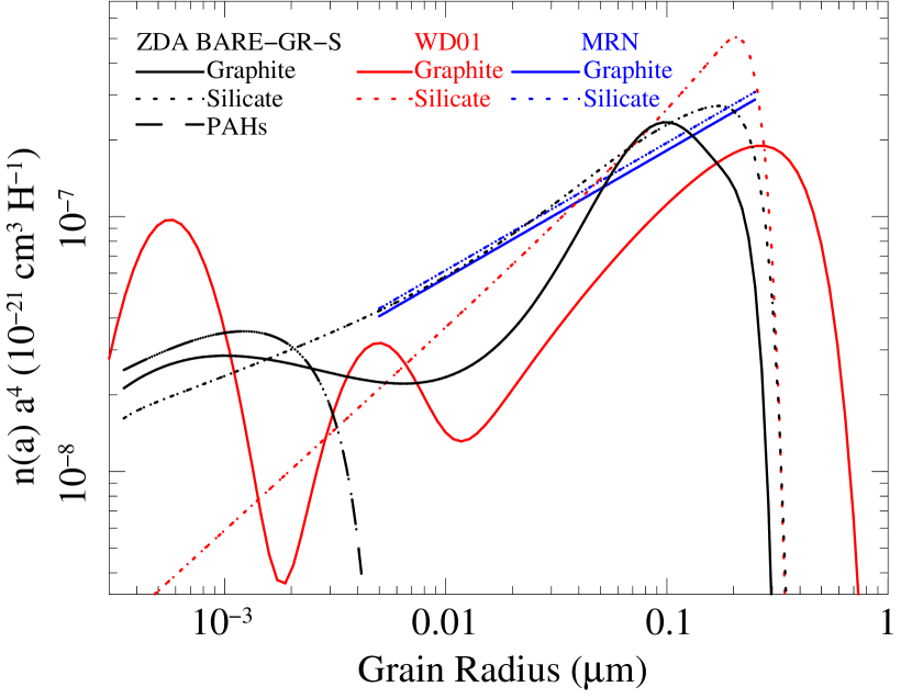
Figure 3.— Example grain-size distributions for the MRN, WD01, and the ZDA BARE-GR-S dust models.

Based on a detailed analysis of observed XAFS (X-ray Absorption Fine Structure) in Cygnus X-1 spectra of the Fe L band (Lee et al., 2009a, 2011) using the techniques described in Lee et al. (2009b, see also ), we introduce an additional model, which we dub XLNW, where the major Fe-containing grain compound olivine ($\rm FeMgSiO_{4}$) in the ZDA BARE-GR-S model is replaced with an iron grain consisting of a metallic iron core surrounded by troilite (FeS), and enstatite ($\rm MgSiO_{3}$). In generating this new model, for each compound, the normalization coefficient ($A$) is adjusted to meet the criteria of the following dust mass equations (in different representations on both the left and right side)

$$\frac{A_{Z}~{}M}{N_{\rm A}}={{{4}\over{3}}\pi\rho\int_{a_{\rm min}}^{a_{\rm max}}{\rm d}a\,n(a)a^{3}},$$ (6)

where for the grains replacing olivine, $A_{\rm Z}=A_{\rm Mg}=A_{\rm Si}=A_{\rm Fe}$ is the abundance of the dust compound, $M$ is the molecular weight in atomic mass units (AMU), and $N_{\rm A}=6.02\times 10^{23}$ is Avogadro’s constant. As described above, $\rho$, $a$, $a_{\rm min}$, $a_{\rm max}$ and $n(a)$ are, respectively, mass density, radius, minimal radius, maximal radius and size distribution of the dust grains. (The normalization coefficient, $A$, is a parameter contained within $n(a)$.) For the iron compound, i.e., iron metal + troilite ($\rm FeS_{0.6}$), $\rho=5.2~{}{\rm g\,cm^{-3}}$, $A_{Z}=33.3\times 10^{-6}$ and $M=75.2$ AMU while $\rho=3.2~{}{\rm g\,cm^{-3}}$, $A_{Z}=33.3\times 10^{-6}$ and $M=100$ AMU for enstatite ($\rm MgSiO_{3}$). Values for $\rho$ are taken from a mineralogy database; where the compound is an admixture, $\rho$ is taken to be the weighted average of the minerals which make up the compound.

As in the ADA and MRN models, all Fe and Si are assumed to reside in the dust, as borne out also by our XAFS fitting. The particle size distributions of iron dust and enstatite are the same as those of silicate in ZDA BARE-GR-S. The normalization of the size distribution, however, has been slightly changed by adjusting the amount of dust appropriate for the assumed depletion. The size distributions and the normalization coefficient ($A$) of the XLNW dust model are shown in Fig. 4.

3. Observation and Data Analysis

We now will use two Chandra -HETGS observations to study the X-ray halo of Cygnus X-1  using the methods discussed above. The first observation occurred on 1999 October 19 (ObsID 107) and lasted about 15 ks. During this time the source was transiting between its hard, power-law dominated state, and the more thermal soft state (see Schulz et al. 2002 for a study of the source behavior). As is characteristic for black holes in this transitional state, the overall source variability was low. This property allows us to use these data to measure a single non-variable radial halo profile which we use to determine the spatial distribution of the dust grains. The second observation was performed on 2004 April 19 (ObsID 3814). This later observation lasted about 50 ks and was designed by us to be performed during the upper conjunction of the black hole (Hanke et al., 2009). During this orbital phase the X-ray lightcurve is strongly variable due to frequent photoabsorption dips as the line of sight to the black hole crosses through the clumpy focused stellar wind of the companion. Due to dramatic variability, this observation is well-suited to determine the distance to Cygnus X-1 .

We create two datasets, as described below, to perform these analyses. One is a steady spatial/spectral halo radial profile that is used for determining the composition of the halo. This dataset is primarily comprised of ObsId 107, however, we describe a procedure to replace the inner ($<$20 arcsec) data in order to obtain a more accurate profile. The second dataset consists of variable halo lightcurves, as a function of radius, comprised solely of data from ObsID 3814. The latter dataset is used for the distance determination.

Figure 4.— The particle size distributions of our XLNW dust model, which is a modified form of the ZDA BARE-GR-S model.

In order to form the datasets, we follow the same procedure described in Xiang et al. (2007) to extract the HETGS spectra, halo radial profile, and halo lightcurve. (See that paper for a detailed analysis flow chart.) CIAO 4.2 with CALDB 4.2 was used. A theoretical point spread function (PSF) created with the Chandra Ray Tracer (ChaRT; Carter et al. 2003) is used for small angles ($<$60 arcsec). ChaRT has been shown to represent properly the PSF behavior; (Xiang et al., 2007). The PSF obtained from ChaRT simulations, however, is underestimated at large off-axis angles ($\gtrsim 60^{\prime\prime}$). We therefore use the bright and halo-less point source Her X-1 to perform an ab initio determination of the PSF at large angles. Her X-1 was observed on 2002 July 02 (ObsID 3662) with Chandra ACIS-I. The parameters of these three observations are listed in Table 2.

Table 2Parameters of three Chandra  observations

Source	Observation	State	Instrument	Start Time	End Time	Exposure	Usagea
	ID					(ks)
Cyg X-1	107	Transition	AICS-S/HETG	1999-10-19 19:17:37	1999-10-19 23:52:10	11.4	RP
Cyg X-1	3814	Low/Hard	AICS-S/HETG	2003-04-19 16:47:31	2003-04-20 06:41:42	47.2	RP + LC
Her X-1	3663	High/Soft	AICS-S/I	2002-07-01 23:37:38	2002-07-02 14:03:05	49.6	PSF

Both the halo and the PSF represent functions of radius and energy. The PSF specifically is the ratio between the surface brightness, absent a halo, and the point source spectrum. In order to determine the surface brightness associated with the combined halo and PSF, we need an accurate estimate of the source spectrum for both Cyg X-1 observations discussed here. In each of these cases, the spectra extracted from the zeroth-order suffer heavy pileup over the entire energy band and also suffer pileup in the first order gratings spectra above 0.7 keV. We therefore follow the method used by Smith et al. (2002) and Valencic et al. (2009) to extract the spectrum from the readout streak, which is completely pileup free. We then use the simple model – a disk blackbody plus powerlaw coupled with cold gas absorption – that has been used to fit these two observations (Schulz et al., 2002; Hanke et al., 2009). Below 0.7 keV, we use the MEG$\pm$1 spectra, which are pileup free. The flux of Cygnus X-1  is determined from the fit to these joint MEG$\pm 1$ spectra and the readout streak spectra. The transitional state spectra, overplotted with the best fit model, are shown in Fig. 5. (The spectral flux during the hard state is also derived with the same methods.) It should be noted that the $N_{\rm H}$ fit from these spectra contains gas local to the Cygnus X-1  system and therefore is expected to result in $N_{\rm H}$ values higher than those that we expect to obtain from modeling the halo radial profile.

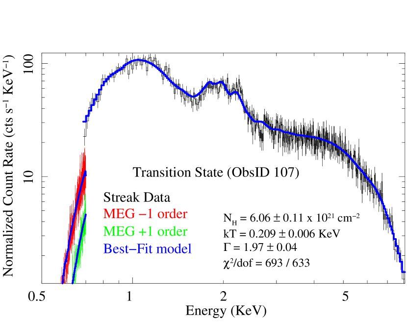
Figure 5.— The streak spectrum and MEG first order spectra overplotted with the best fit model.

As discussed above, ObsID 107 was used to generate the non-variable halo radial profiles. Due to the brightness of Cygnus X-1 during the transitional observation (ObsID 107), however, these data suffer severe pileup at small angles. In order to investigate clouds very near the source, halos at small angles are needed. We therefore excise the core of the halo from ObsID 107 and substitute data from the hard state observation, where due to its low flux, pileup free halos can be extended to as low as $7^{\prime\prime}$ radius. In this work, the total surface brightness (see Fig. 6) at greater than 20 arcsec radius is extracted from the transitional state observation (ObsID 107), while the surface brightness at less than 20 arcsec radius is from the hard state (ObsID 3814). Even though Cygnus X-1  is variable, this approach is justified since at small angles the time delay between the source and the halo is negligible, and we therefore can compare the time averaged source flux to the time averaged radial profiles.

To determine the energy dependent halo profile using these data, we extracted the halo and PSF radial profiles in energy bands of 200 eV width over the range 0.4–10.0 keV. That is, we use bands that correspond roughly to the energy resolution of ACIS-I/S, which varies from 100 to 200 eV in this range. We find that above 4.0 keV, the halo intensity is much smaller than the PSF intensity (i.e., the surface brightness attributable to the point source). Additionally, the Rayleigh-Gans approximation underestimates the halo intensity below 1.0 keV (Smith & Dwek, 1998). We therefore only use the halo from 1.0 keV to 4.0 keV in the following. The total surface brightness (Halo + PSF), PSF, and PSF-subtracted net halo profiles are shown in Fig. 6 for the 2–2.2 keV band. In this band, at angular distances greater than $10^{\prime\prime}$, the halo surface brightness is significantly larger than the surface brightness of the point source (i.e., the PSF intensity). On the other hand, for all energies $>$1.6 keV and angular distances $<10^{\prime\prime}$ the data are fully dominated by the point source and therefore are ignored in the following study. For energies below 1.6 keV we can approach the point source to separations as low as $7^{\prime\prime}$. At smaller angular separations the pileup ratio is greater than $\>5\%$ and the data have to be ignored at all energies.

A final complication arises for energies above 2.0 keV and radial distances $>200^{\prime\prime}$. Here, the halo profile is contaminated by photons from the $1^{\mathrm{st}}$ order gratings spectrum. Of special importance are photons in the MEG$\pm$$1^{\mathrm{st}}$ order, which starts closer to the zeroth order than the HEG$\pm$$1^{\mathrm{st}}$ order spectrum. We therefore ignored the halo radial profile at $>200^{\prime\prime}$ for energies above 2.0 keV.

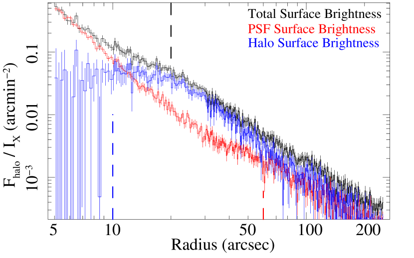
Figure 6.— Comparison of the radial profiles between the halo and the PSF (i.e., the surface brightness attributable solely to the point source) in the 2.0–2.2 keV energy band. The total surface brightness (black) was created from a combination of ObsID 3814 ($<$20 arcsec) and ObsID 107 ($>$20 arcsec). – A vertical black dashed line delineates these two regions. The PSF profile was created from ChaRT simulations ($<$60 arcsec) and from a non-variable Her X-1 observation ($>60$ arcsec). Data from less than $10$ arcsec (marked by vertical blue dashed line) is not considered in this energy band.

4. Spatial Distribution of Dust Grains

For our initial modeling, dust uniformly distributed along the entire LOS was assumed. This approach did not result in satisfactory descriptions of the halo radial profile observations using any of the 18 dust models. Following the method of Xiang et al. (2005, 2007), we therefore assume an inhomogeneous dust distribution along the line of sight. We divide the LOS into 10 approximately logarithmically spaced bins. That is, the spatial resolution of the dust distribution increases towards the source. The relative density distribution along the LOS as derived from fits to the halo radial profile and assuming the ZDA BARE-GR-S model is shown in Fig. 7. The ZDA BARE-GR-S model gave the best fits for the reddening of 4U 1724$-$307 in the work by Valencic et al. (2009) and it is also one of our favored models (see Section 6).

The data prefer approximately three regions of different characteristic densities. The highest density region is found at a relative distance between $\approx 0.84$–0.94. The regions extending from $\approx 0.94$–1.0 and from $\approx 0.0--0.6$ exhibited lower columns. Similar results were obtained when using 10 linearly spaced bins (inset of Fig. 7): there was little column between 0.0–0.8, and the bins between 0.8–0.9 and 0.9–1.0 have different characteristic densities.

In the ensuing analysis, we discuss these three characteristic regions as if they were three individual clouds. Furthermore, we label these three regions, starting near us and working outwards towards the source, as Cloud Obs, Cloud Mid, and Cloud Src. Cloud Mid contributes more than 50% of the total dust grains along the LOS. This result is consistent with Ling et al. (2009), who use a cross-correlation method to derive the position of this dominant cloud from the delay time of the scattered photons.

Figure 7.— Relative density distributions along the LOS based on halo radial profile fits using the ZDA BARE-GR-S dust model. The observer is at 0, and the source is at 1. A cloud at $\sim$0.88 is obvious. The inset (a) figure (in blue) also shows a cloud near the source when ten linear-equally spaced bins are instead used in the model. (In subsequent discussion and fits presented below, a simplified three-zone model, inspired by the above results, is used.)

Figure 2 shows that the halo flux between $20^{\prime\prime}$ and $45^{\prime\prime}$ is dominated by photons scattered by Cloud Mid. The delay time of scattered photons depends especially strongly on the distance of this cloud. To make the calculation of the predicted distances and fitting of the halo lightcurves more tractable, we further simplify the description of the dust spatial distribution. Specifically, based upon the preliminary radial profile fit shown in Fig. 7 that exhibits three regions with different characteristic densities, we formally divide the LOS into three components. Uniform density regions are used to represent Cloud Obs between 0.0–$x_{\mathrm{o}}$, Cloud Src between $x_{\mathrm{s}}$–1.0, and Cloud Mid centered at $x_{\mathrm{c}}$. Ling et al. (2009) claimed limits on the width of this latter, dominant cloud of $\Delta x=0.016_{-0.006}^{+0.009}$; therefore, in this work we have adopted a fixed width of 0.016 ($\sim$30 pc). We reexamine this limit in §5, where we show that a cloud with a large extent does not fit the dust scattering halo lightcurves. For convenience, we take the upper limit to be $x=1$; however, it should be noted that the dust located very near the source, i.e, $x>0.99$, might be contaminated by the wind of HDE 226868, the companion of Cygnus X-1 . Note that the halo scattered by this dust is concentrated at very small angles ($<$$7^{\prime\prime}$) and contributes very little to the portion of the halo considered in this work. We therefore still use the same dust model along the entire LOS. We have also checked that changing the upper limit of Cloud Src to $x=0.99$ from $x=1.0$ does not provide significantly different results for the $N_{\rm H}$ due to the Cloud Src nor does it affect the distance determination.

The relative distances $x_{\mathrm{o}}$, $x_{\mathrm{c}}$, and $x_{\mathrm{s}}$ were initially allowed to vary in our fits. We found that both the total hydrogen column density and the position of Cloud Mid, i.e., $x_{\mathrm{c}}$, are not greatly affected by variations of $x_{\mathrm{o}}$ but are strongly correlated with the value of $x_{\mathrm{s}}$. The former fact is not surprising given the low relative density in this region close to the observer, as shown in Fig. 7. For the following halo radial profile fits we therefore fix $x_{\mathrm{o}}$ to 0.70, which is the best fit value for the model of ZDA BARE-GR-S. On the other hand, $x_{\mathrm{s}}$ was allowed to vary between 0.75–0.98. The eighteen dust grain models described in Section 2.3 — MRN, WD01, 15 ZDA models, and our XLNW model — are used to fit the halo radial profile.

When the XLNW dust model is used to fit the halo radial profiles, we derive a scattering hydrogen column density that is consistent with the absorption hydrogen column density derived from XAFS studies (Lee et al., 2011). It should be noted that our XLNW model yields a similar position for Cloud Mid as do the BARE-GR-S, and BARE-GR-FG. These latter models also yield scattering hydrogen column densities consistent with the XAFS studies.

We now turn to using the above preliminary fits to the halo radial profile to constrain the fitting of the halo lightcurves.

5. Distance Determination

The halo lightcurves of Cygnus X-1  clearly show significant delays with respect to the source lightcurves. The delay time strongly depends on the observed off-axis angles. In order to measure the delay, we calculate halo light curves for six, $5^{\prime\prime}$ wide annuli, with the inner radii ranging from $20$–$45^{\prime\prime}$. Outside this interval, the delay times exceed the duration of our observation.

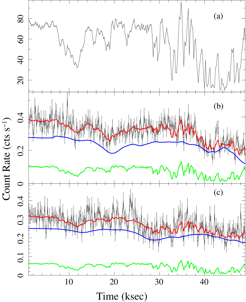
Figure 8.— Point source lightcurves and lightcurves at a given annulus, in the 1–4 keV band, overplotted by the best-fit models (red) using the ZDA BARE-GR-S dust model. The blue line indicates the lightcurves derived from the dust model, while the green line is the modeled PSF lightcurve. Their sum yields the red lightcurve. The top panel (a) is the central point source lightcurve. The middle panel (b) is the 20–$25^{\prime\prime}$ annulus. The bottom panel (c) is the 30–$35^{\prime\prime}$ annulus.

Following the method of Xiang et al. (2005), we use the derived dust spatial distribution to fit the halo lightcurves with the absolute distance to the source being the free parameter. The best-fit distance is determined by minimizing $\chi^{2}$ based on simultaneously fitting the delays in all lightcurves. Figure 8 shows the point source and halo lightcurves overplotted with the best-fit of the ZDA BARE-GR-S model, using a single fit distance for all lightcurves considered simultaneously.

The time delayed lightcurves also carry information about the positions of the clouds such that the lightcurve fits also can be used to constrain the position of $x_{\mathrm{s}}$ further than by just using the halo profile. We therefore vary $x_{\mathrm{s}}$ from 0.75 to 0.98, and at each trial value of $x_{\mathrm{s}}$ we perform a constrained fit to the radial profile to determine $x_{\mathrm{c}}$ and the hydrogen column densities. We then use these radial profile derived parameters to fit the halo lightcurves and obtain a minimum $\chi^{2}$. While the $\chi^{2}$ from solely a fit of the halo radial profile varies little with $x_{\mathrm{s}}$, the $\chi^{2}$ from fits of the halo lightcurve varies significantly with $x_{\mathrm{s}}$. We use this variation in $\chi^{2}$ to create a lightcurve determined uncertainty for $x_{\mathrm{s}}$ (i.e., $\Delta\chi^{2}=2.71$ to determine the 90% error bars). For 13 of the 18 dust grain models, the values of $x_{\mathrm{s}}$ derived from the preliminary radial profile fits described above and those values derived from the lightcurves were self-consistent with one another, i.e., the 90% error bars for each estimate (lightcurve, radial profile) of $x_{\mathrm{s}}$ significantly overlapped.

Given that the iterative approach to fitting the radial profile and then fitting the lightcurve failed to produce self-consistent fit parameters for five cases, we then turned to a joint fit of these data. Specifically, we used the solutions obtained from the iterative approach as starting parameter values, and then simultaneously fit the radial profile and the lightcurve data with six variable parameters: $x_{\mathrm{s}}$, $x_{\mathrm{c}}$, $d$, and three hydrogen column densities, $N_{\rm H}^{\rm mid}$, $N_{\rm H}^{\rm obs}$, and $N_{\rm H}^{\rm src}$. The results of these fits are presented in Table 3. The $N_{\rm H}^{\rm tot}$ are the sum of $N_{\rm H}^{\rm mid}$, $N_{\rm H}^{\rm obs}$, and $N_{\rm H}^{\rm src}$. The iron column density $N_{\rm Fe}^{\rm tot}$ is derived from $N_{\rm tot}^{\rm H}$ based on the iron abundance for each dust model (see Table 1). Parameter uncertainties are given as the 90% confidence level for one interesting parameter, i.e., $\Delta\chi^{2}=2.71$ for fits holding the parameter of interest frozen at a given value. Values of $x_{\mathrm{s}}$, $x_{\mathrm{c}}$, $N_{\rm Fe}^{\rm tot}$, and $d$ for each dust model are presented in Fig. 9.

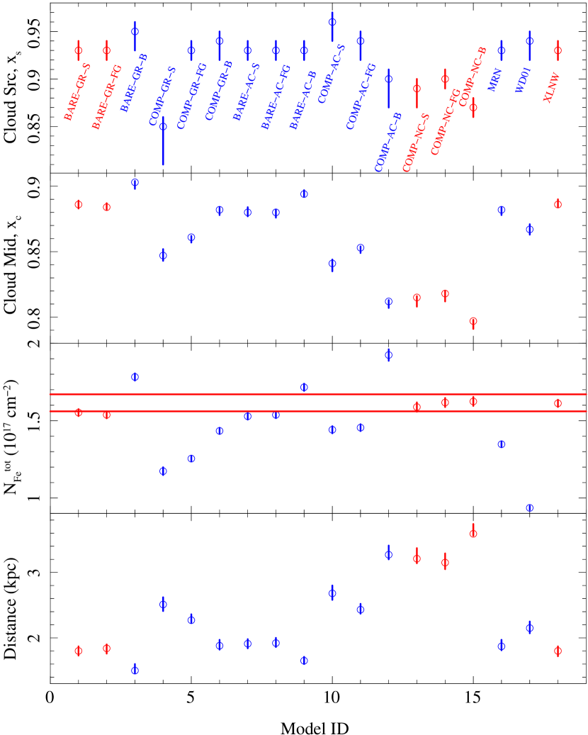
Figure 9.— The results of the joint fits to the halo radial profile and lightcurve for each model. (Model ID is shown along the $x$-axis, and model names are given in the top panel.) The top two panels give the relative positions of the cloud nearest the source ($x_{\mathrm{s}}$), and the next closest cloud ($x_{\mathrm{c}}$). The next panel gives the summed total neutral column (converted to an equivalent Fe column based on the respective olivine abundance listed in Table 1 for each dust model) for all of the clouds between us and the source. The two red lines show the iron column estimate obtained from the Lee et al. (2011) modeling of the $\sim$700 eV FeL absorption edges and associatd XAFS in HETGS spectra of Cygnus X-1 . For all panels, models plotted in red agree with the neutral column density estimate based on iron. The bottom panel gives the best fit source distance for each model. The median value is 1.82 kpc, while three of the six models that agree with the neutral column estimates of Lee et al. (2011) give distance estimates that lie in the range from 1.72–1.90 kpc.

Our derived scattering dust iron column density varies from $0.94\times 10^{17}\rm\ cm^{-2}$ to $1.92\times 10^{17}\rm\ cm^{-2}$, which should be equal to the Galactic absorption dust iron column density. We therefore use results from absorption spectra to constrain further the dust models. We choose to compare to the iron column density as it can be measured directly via modeling of the Fe L edge in high spectral resolution data (Hanke et al., 2009; Lee et al., 2009a, 2011). As discussed by Wilms et al. (2000), neutral column absorption in the X-rays is dominated by $Z>2$ elements, i.e., not hydrogen. Comparing directly to the X-ray derived Fe column therefore removes the ambiguity of the assumed elemental abundances relative to hydrogen in such spectral models.

The total absorption iron column density of Cyg X-1 derived from absorption spectra varies from $0.96\times 10^{17}\rm\ cm^{-2}$ (Juett et al., 2006) to $2.52\times 10^{17}\rm\ cm^{-2}$ (Hanke et al., 2009). Aside from possible instrumental differences, these different values are in part due to variations in the column density local to the source, e.g., because of absorption in the stellar wind (see Hanke et al., 2009), as well as variations in the assumed absorption cross sections. Our recent studies of observed X-ray Absorption Fine Structure (XAFS) in the Low/Hard, Transition, and High/Soft states (Lee et al., 2011) suggest that the dust iron column density associated with Cyg X-1 is $1.62\pm 0.06\times 10^{17}\ \rm cm^{-2}$. Only six of the eighteen dust models considered for the halo modeling have $N_{\mathrm{Fe}}$ consistent with this value. (The parameters for these models are plotted in red in Fig. 9.) Of these six models, three models, ZDA BARE-GR-S, ZDA BARE-GR-FG, and our proposed model XLNW, yield source distances that lie in the range from 1.72–1.90 kpc (The median distance for all three models is 1.82 kpc.), whereas three models, ZDA ZDA COMP-NC-S, ZDA COMP-NC-FG and ZDA COMP-NC-B, yield larger distances of 3.15–3.59 kpc. The large distance values for these latter three models, compared to the most recent distance estimates (discussed below) leads us to discount these fits. This leaves us with three models that we favor to describe the halo and absorption profile of Cygnus X-1 .

Figure 10.— The distances derived from lightcurves at different radii for one thin cloud (a), one thick cloud (b), and two thin clouds (c). Only the distances derived from one thin cloud are consistent with each other for each radii. The dashed horizontal lines indicate the average distance. The uncertainties in this figure are only from the fits to the halo lightcuves. The error bars in this figure are only 1$\sigma$. Additional uncertainties from uncertainties in the radial profile fits are not included.

Lastly we consider the possibility that the cloud with a relative distance between 0.8 and 0.9 is a thick cloud, or that the cloud might be divided into 2 parts. For the first possibility, we set a cloud with a width of 0.1 (relative distance) located at $x_{\mathrm{c}}=0.878$. This location is the best fit value of $x_{\mathrm{c}}$ derived from radial profile fits using the ZDA BARE-GR-S model. The distances then fitted from halo lightcurves at different angles are then not consistent with each other, as shown in the middle panel of Fig. 10. For the second possibility, we locate one thin cloud at 0.85 and another thin cloud at 0.90. The width of each cloud is set to 0.016. The distances fitted from individual halo lightcurves are again found to be inconsistent with each other, as shown in the bottom panel of Fig. 10. We also noticed that the $\chi^{2}/$DoF of the distance fit with thick cloud ($\chi^{2}/$DoF = 1003/777) or two thin clouds ($\chi^{2}/$DoF = 983/776) is much worse than that from one thin cloud fit ($\chi^{2}/$DoF = 884/777). This further justifies our assumption of a single thin cloud at the position $x_{\mathrm{c}}$.

6. Discussion and Summary

Using the X-ray dust scattering halo radial profiles and lightcurves combined with the X-ray absorption hydrogen column density, we can begin to distinguish among the dust grain models. Our favored dust models are BARE-GR-S, BARE-GR-FG, and XLNW. It should be noted that the first two models, i.e., BARE-GR-S and BARE-GR-FG, also yield the proper optical extinction for the LOS to the X-ray binary 4U 1724$-$307 (Valencic et al., 2009). Our fits using the classic MRN model and the more recent model of WD01 underestimated the hydrogen column density to Cygnus X-1 ; similar underestimates with these two models were found by Valencic & Smith (2008) for X Persei and Valencic et al. (2009) for 4U 1724$-$307. All three of our favored models contain graphite, while none of the dust models containing amorphous carbon simultaneously yield good neutral columns and source distances (see below). This result suggests that carbon in the ISM prefers to reside in graphite instead of amorphous carbon dust. Our proposed model XLNW, which separates iron from olivine, can yield a proper hydrogen column density and a proper position for the source, as discussed below.

Our results show that the dust scattering halo radial profiles together with the halo lightcurve provide a potentially powerful tool to determine the relative position of the cloud along the LOS, and to determine the geometric distance to the point source. All three of our favored models show that Cloud Src is located at $x_{\mathrm{s}}\sim$0.92–0.95 and that Cloud Mid is located at $x_{\mathrm{c}}\approx 0.885$. Our fitted distances to Cygnus X-1  for the most part lie within a narrow range of 1.72–1.90. This distance range is consistent with recent radio parallax measurements for Cygnus X-1  which yield a distance of $d=1.86\pm 0.12$ kpc (Reid et al., 2011). This is considered the most reliable method to determine the distance. The distance derived from our proposed dust model containing iron metal and troilite is consistent with those derived from BARE-GR-S and BARE-GR-FG, both of which yield the proper column density.

The first estimate of the distance to Cygnus X-1  was made by Margon et al. (1973) using the surveyed optical extinction in the field immediately surrounding Cygnus X-1 . The distance of $d=2.5\pm 0.4$ kpc was confirmed by Ninkov et al. (1987) and was used by many researchers. Russell et al. (2007) and Gallo et al. (2005) imply that Sharpless 2-101 hereafter Sh 2-101, which is is a bright reflection nebula to the north east of Cygnus X-1 , is close to Cygnus X-1 . Russell et al. (2007) also suggest that the nebula interacts with the jet of Cygnus X-1 . The distance of Sh 2-101 is generally assumed to be larger than 2.2 kpc. Our results, most of which are significantly lower than 2.2 kpc, hint that Sh 2-101 is a background source and therefore the Cygnus X-1  jet is not interacting with it. Alternatively, measurements of the distance to Sh 2-101 may be overestimates.

Table 3Distances, cloud positions, and $N_{\rm H}$ from global fits.

Model	Model	Cloud Srca	Cloud Midb	Distance	$N_{\rm H}^{{\rm mid}}$	$N_{\rm H}^{{\rm obs}}$	$N_{\rm H}^{{\rm src}}$	$N_{\rm H}^{{\rm tot}}$	$N_{\rm Fe}^{{\rm tot}}$	$\chi^{2}/DoF$
No	Name	Position ($x_{s}$)	Position ($x_{c}$)	(kpc)	$(\rm 10^{21}~{}cm^{-2})$				$(\rm 10^{17}~{}cm^{-2})$
1	BARE-GR-S	$0.93_{-0.01}^{+0.01}$	$0.886_{-0.003}^{+0.003}$	$1.80_{-0.07}^{+0.07}$	$2.47_{-0.04}^{+0.04}$	$1.42_{-0.05}^{+0.05}$	$0.77_{-0.03}^{+0.03}$	$4.66_{-0.07}^{+0.07}$	$1.55_{-0.02}^{+0.02}$	4277/3969
2	BARE-GR-FG	$0.93_{-0.01}^{+0.01}$	$0.884_{-0.002}^{+0.003}$	$1.84_{-0.08}^{+0.06}$	$2.45_{-0.04}^{+0.04}$	$1.40_{-0.04}^{+0.05}$	$0.80_{-0.04}^{+0.04}$	$4.65_{-0.07}^{+0.07}$	$1.54_{-0.02}^{+0.02}$	4279/3969
3	BARE-GR-B	$0.95_{-0.02}^{+0.01}$	$0.903_{-0.005}^{+0.001}$	$1.50_{-0.04}^{+0.10}$	$3.32_{-0.04}^{+0.04}$	$2.05_{-0.06}^{+0.06}$	$0.88_{-0.03}^{+0.03}$	$6.25_{-0.08}^{+0.08}$	$1.78_{-0.02}^{+0.02}$	4291/3969
4	COMP-GR-S	$0.85_{-0.04}^{+0.01}$	$0.847_{-0.004}^{+0.005}$	$2.51_{-0.10}^{+0.11}$	$1.78_{-0.05}^{+0.04}$	$1.08_{-0.03}^{+0.04}$	$0.70_{-0.05}^{+0.05}$	$3.56_{-0.08}^{+0.08}$	$1.17_{-0.02}^{+0.03}$	4262/3969
5	COMP-GR-FG	$0.93_{-0.01}^{+0.01}$	$0.861_{-0.004}^{+0.001}$	$2.27_{-0.04}^{+0.09}$	$2.18_{-0.03}^{+0.03}$	$1.17_{-0.03}^{+0.04}$	$0.52_{-0.04}^{+0.04}$	$3.87_{-0.06}^{+0.06}$	$1.25_{-0.02}^{+0.02}$	4253/3969
6	COMP-GR-B	$0.94_{-0.02}^{+0.01}$	$0.882_{-0.004}^{+0.002}$	$1.88_{-0.06}^{+0.09}$	$2.85_{-0.04}^{+0.04}$	$1.61_{-0.05}^{+0.05}$	$0.70_{-0.04}^{+0.04}$	$5.16_{-0.07}^{+0.07}$	$1.43_{-0.02}^{+0.02}$	4251/3969
7	BARE-AC-S	$0.93_{-0.01}^{+0.01}$	$0.880_{-0.003}^{+0.004}$	$1.91_{-0.07}^{+0.07}$	$2.32_{-0.03}^{+0.03}$	$1.47_{-0.04}^{+0.04}$	$0.77_{-0.04}^{+0.04}$	$4.56_{-0.06}^{+0.06}$	$1.53_{-0.02}^{+0.02}$	4280/3969
8	BARE-AC-FG	$0.93_{-0.01}^{+0.01}$	$0.880_{-0.004}^{+0.002}$	$1.92_{-0.06}^{+0.08}$	$2.27_{-0.03}^{+0.03}$	$1.48_{-0.04}^{+0.04}$	$0.75_{-0.04}^{+0.04}$	$4.50_{-0.06}^{+0.06}$	$1.54_{-0.02}^{+0.02}$	4277/3969
9	BARE-AC-B	$0.93_{-0.01}^{+0.01}$	$0.894_{-0.002}^{+0.003}$	$1.65_{-0.05}^{+0.06}$	$2.85_{-0.04}^{+0.04}$	$2.09_{-0.06}^{+0.06}$	$1.04_{-0.04}^{+0.04}$	$5.98_{-0.08}^{+0.08}$	$1.72_{-0.02}^{+0.02}$	4295/3969
10	COMP-AC-S	$0.96_{-0.02}^{+0.01}$	$0.841_{-0.006}^{+0.003}$	$2.68_{-0.10}^{+0.12}$	$2.61_{-0.03}^{+0.03}$	$1.26_{-0.04}^{+0.04}$	$0.46_{-0.05}^{+0.05}$	$4.33_{-0.07}^{+0.07}$	$1.44_{-0.02}^{+0.02}$	4263/3969
11	COMP-AC-FG	$0.94_{-0.02}^{+0.01}$	$0.853_{-0.004}^{+0.001}$	$2.43_{-0.06}^{+0.09}$	$2.49_{-0.03}^{+0.03}$	$1.32_{-0.04}^{+0.04}$	$0.51_{-0.04}^{+0.04}$	$4.32_{-0.06}^{+0.06}$	$1.45_{-0.02}^{+0.02}$	4254/3969
12	COMP-AC-B	$0.90_{-0.03}^{+0.01}$	$0.812_{-0.005}^{+0.001}$	$3.27_{-0.07}^{+0.14}$	$4.43_{-0.07}^{+0.07}$	$1.31_{-0.08}^{+0.08}$	$1.16_{-0.08}^{+0.08}$	$6.90_{-0.13}^{+0.13}$	$1.92_{-0.04}^{+0.04}$	4289/3969
13	COMP-NC-S	$0.89_{-0.02}^{+0.01}$	$0.815_{-0.007}^{+0.001}$	$3.21_{-0.07}^{+0.16}$	$2.82_{-0.05}^{+0.05}$	$1.25_{-0.05}^{+0.05}$	$0.68_{-0.06}^{+0.06}$	$4.75_{-0.09}^{+0.09}$	$1.59_{-0.03}^{+0.03}$	4285/3969
14	COMP-NC-FG	$0.90_{-0.01}^{+0.01}$	$0.818_{-0.006}^{+0.002}$	$3.15_{-0.10}^{+0.14}$	$2.84_{-0.05}^{+0.05}$	$1.32_{-0.05}^{+0.05}$	$0.61_{-0.06}^{+0.05}$	$4.77_{-0.09}^{+0.09}$	$1.62_{-0.03}^{+0.03}$	4282/3969
15	COMP-NC-B	$0.87_{-0.01}^{+0.01}$	$0.797_{-0.006}^{+0.001}$	$3.59_{-0.03}^{+0.15}$	$3.07_{-0.06}^{+0.06}$	$1.64_{-0.06}^{+0.06}$	$1.06_{-0.06}^{+0.06}$	$5.78_{-0.10}^{+0.10}$	$1.62_{-0.03}^{+0.03}$	4285/3969
16	MRN	$0.93_{-0.01}^{+0.01}$	$0.882_{-0.004}^{+0.002}$	$1.87_{-0.06}^{+0.10}$	$2.07_{-0.03}^{+0.03}$	$1.27_{-0.04}^{+0.04}$	$0.74_{-0.03}^{+0.03}$	$4.08_{-0.06}^{+0.06}$	$1.35_{-0.02}^{+0.02}$	4303/3969
17	WD01	$0.94_{-0.02}^{+0.01}$	$0.867_{-0.004}^{+0.004}$	$2.15_{-0.08}^{+0.10}$	$1.39_{-0.02}^{+0.02}$	$0.84_{-0.02}^{+0.02}$	$0.35_{-0.02}^{+0.02}$	$2.58_{-0.04}^{+0.04}$	$0.94_{-0.01}^{+0.01}$	4259/3969
18	XLNW	$0.93_{-0.01}^{+0.01}$	$0.886_{-0.002}^{+0.004}$	$1.80_{-0.08}^{+0.07}$	$2.56_{-0.04}^{+0.04}$	$1.47_{-0.05}^{+0.05}$	$0.81_{-0.04}^{+0.04}$	$4.84_{-0.07}^{+0.07}$	$1.61_{-0.02}^{+0.02}$	4277/3969

References

- Canizares et al. (2005) Canizares, C. R., et al., 2005, PASP, 117, 1144
- Carter et al. (2003) Carter, C., Karovska, M., Jerius, D., Glotfelty, K, & Beikman, S., 2003, ADASS XII, ASP Conference Series Vol. 295, eds. H.E. Payne, R.I. JEdzrejewski, & R.N. Hook, 477.
- Costantini et al. (2005) Costantini, E., Freyberg, M. J., & Predehl, P. 2005, A&A, 444, 187
- Gallo et al. (2005) Gallo, E., Fender, R., Kaiser, C., Russell, D., Morganti, R., Oosterloo, T., & Heinz, S. 2005, Nature, 436, 819
- Garmire et al. (2003) Garmire, G. P., Bautz, M. W., Ford, P. G., Nousek, J. A., & Ricker, Jr., G. R., 2003, in Society of Photo-Optical Instrumentation Engineers (SPIE) Conference Series, ed. J. E. Truemper & H. D. Tananbaum, Vol. 4851, 28
- Hanke et al. (2009) Hanke, M., Wilms, J., Nowak, M. A., Pottschmidt, K., Schulz, N. S., & Lee, J. C. 2009, ApJ, 690, 330
- Henke (1981) Henke, B. L. 1981, in American Institute of Physics Conference Series, Vol. 75, Low Energy X-ray Diagnostics, ed. D. T. Attwood & B. L. Henke, 146–155
- Juett et al. (2006) Juett, A. M., Schulz, N. S., Chakrabarty, D., & Gorczyca, T. W. 2006, ApJ, 648, 1066
- Lee (2010) Lee, J. C., 2010, Space Science Reviews, 157, 93
- Lee et al. (2001) Lee, J. C., Ogle, P. M., Canizares, C. R., Marshall, H. L., Schulz, N. S., Morales, R., Fabian, A. C., & Iwasawa, K., 2001, Astrophys. J., Lett., 554, L13
- Lee et al. (2009a) Lee, J. C., et al., 2009a, in Astro2010: The Astronomy and Astrophysics Decadal Survey, Vol. 2010, 178
- Lee et al. (2009b) Lee, J. C., Xiang, J., Ravel, B., Kortright, J., & Flanagan, K., 2009b, ApJ, 702, 970
- Lee et al. (2011) Lee, J. C. et al. 2011, in preparation.
- Lestrade et al. (1999) Lestrade, J., Preston, R. A., Jones, D. L., Phillips, R. B., Rogers, A. E. E., Titus, M. A., Rioja, M. J., & Gabuzda, D. C. 1999, A&A, 344, 1014
- Ling et al. (2009) Ling, Z., Zhang, S. N., Xiang, J., & Tang, S. 2009, ApJ, 690, 224
- Margon et al. (1973) Margon, B., Bowyer, S., & Stone, R. P. S. 1973, ApJ, 185, L113
- Mathis et al. (1995) Mathis, J. S., Cohen, D., Finley, J. P., & Krautter, J. 1995, ApJ, 449, 320
- Mathis & Lee (1991) Mathis, J. S., & Lee, C. 1991, ApJ, 376, 490
- Mathis et al. (1977) Mathis, J. S., Rumpl, W., & Nordsieck, K. H. 1977, ApJ, 217, 425
- Mauche & Gorenstein (1984) Mauche, C., & Gorenstein, P. 1984, in Bulletin of the American Astronomical Society, Vol. 16, 926
- Ninkov et al. (1987) Ninkov, Z., Walker, G. A. H., & Yang, S. 1987, ApJ, 321, 425
- Overbeck (1965) Overbeck, J. W. 1965, ApJ, 141, 864
- Predehl et al. (2000) Predehl, P., Burwitz, V., Paerels, F., & Trümper, J. 2000, A&A, 357, L25
- Predehl & Klose (1996) Predehl, P., & Klose, S. 1996, A&A, 306, 283
- Predehl & Schmitt (1995) Predehl, P., & Schmitt, J. H. M. M. 1995, A&A, 293, 889
- Reid et al. (2011) Reid, M. J., McClintock, J. E., Narayan, R., Gou, L. Remillard, R. A. & Orosz, J. A. 2011, Science, submitted.
- Rolf (1983) Rolf, D. P. 1983, Nature, 302, 46
- Russell et al. (2007) Russell, D. M., Fender, R. P., Gallo, E., & Kaiser, C. R. 2007, MNRAS, 376, 1341
- Schulz et al. (2002) Schulz, N. S., Cui, W., Canizares, C. R., Marshall, H. L., Lee, J. C., Miller, J. M., & Lewin, W. H. G. 2002, ApJ, 565, 1141
- Smith & Dwek (1998) Smith, R. K., & Dwek, E. 1998, ApJ, 503, 831
- Smith et al. (2002) Smith, R. K., Edgar, R. J., & Shafer, R. A. 2002, ApJ, 581, 562
- Thompson & Rothschild (2009) Thompson, T. W. J., & Rothschild, R. E. 2009, ApJ, 691, 1744
- Trümper & Schönfelder (1973) Trümper, J., & Schönfelder, V. 1973, A&A, 25, 445
- Valencic & Smith (2008) Valencic, L. A., & Smith, R. K. 2008, ApJ, 672, 984
- Valencic et al. (2009) Valencic, L. A., Smith, R. K., Dwek, E., Graessle, D., & Dame, T. M. 2009, ApJ, 692, 502