Estimating Form Factors of $B_{s}\rightarrow D_{s}^{(*)}$ and their
Applications to Semi-leptonic and Non-leptonic Decays

Abstract

$B_{s}^{0}\rightarrow D_{s}^{-}$ and $B_{s}^{0}\rightarrow D_{s}^{*-}$ weak transition form factors are estimated for the whole physical region with a method based on an instantaneous approximated Mandelstam formulation of transition matrix elements and the instantaneous Bethe-Salpeter equation. We apply the estimated form factors to branching ratios, CP asymmetries and polarization fractions of non-leptonic decays within the factorization approximation. And we study the non-factorizable effects and annihilation contributions with the perturbative QCD approach. The branching ratios of semi-leptonic $B_{s}^{0}\rightarrow D_{s}^{(*)-}l^{+}\nu_{l}$ decays are also evaluated. We show that the calculated decay rates agree well with the available experimental data. The longitudinal polarization fraction of $B_{s}\rightarrow D_{s}^{*}V(A)$ decays are $\sim 0.8$ when $V(A)$ denotes a light meson, and are $\sim 0.5$ when $V(A)$ denotes a $D_{q}$ ($q=d,s$) meson.

1 Introduction

In the past few years, charmless non-leptonic $B_{s}$ decays have been extensively studied [1], however, the decays of $B_{s}$ to charmed particles are relatively less studied. Therefore, it is of urgent interest to put more attention on this topic. Semi-leptonic $B_{s}^{0}\rightarrow D_{s}^{(*)-}l^{+}\nu_{l}$ decays and non-leptonic ${B}^{0}_{s}\rightarrow D_{s}^{(*)-}X^{+}$ two body decays (and their conjugated ones), where $X^{+}$ denotes a light meson or a $D_{q}$ ($q=d,s$) meson, can reveal useful information about the Cabibbo-Kobayashi-Maskawa (CKM) phases, the $B_{s}^{0}-\bar{B}_{s}^{0}$ mixing parameters [2, 3], and the physics of CP violations [4]. Studies on $B_{s}$ decays to charmed particles can be used to check the factorization hypothesis [5] and to search for physics beyond the Standard Model (SM) [6, 7, 8].

For weak decays, the transition form factors play an important role. Theoretically, to estimate the form factors of a relevant process, one has to rely on some non-perturbative approaches such as the Bethe-Salpeter (B-S) equation, quark models, QCD sum rules (QCDSR) and lattice QCD. Turn to $B_{s}\rightarrow D_{s}^{(*)}$ weak transitions, several works have been done: Early works, $e.g.$ [9, 10], usually relied on the famous Bauer-Stech-Wirbel (BSW) model [11]. Authors of [12, 13] adopted QCDSR for the calculation. In [14], the form factors are estimated within the covariant light-front quark model (CLFQM). Authors of [15] used the so called light cone sum rules (LCSR) to investigate form factors at large recoil, and heavy quark effective theory (HQET) to describe them at small recoil region. Each of these methods sketches one or another profile of non-perturbative QCD, and each has advantages as well as shortcomings. So it is worthy to estimate the $B_{s}\rightarrow D_{s}^{(*)}$ form factors in another method which is based on the B-S equation [16] and the Mandelstam formulation [17] of the transition matrix element. To make predictions on non-leptonic decays, there is another task, that is how to evaluate the decay amplitudes with form factors available. It is well known that factorization approximation (FA) [11] has been extensively applied in non-leptonic weak decays and has been justified to success in explaining the branching ratios of several color-allowed $B_{q}$ decays [18]. The works mentioned before all adopted the FA to evaluate non-leptonic decay amplitudes. However, estimations based on the FA still suffer uncertainties from the non-factorizable effects and annihilation diagrams contributions, especially for the CP asymmetries (CPAs). Thus approaches beyond the FA are in need. Till now several approaches which can cover the non-factorizable effects have been developed, such as the perturbative QCD (pQCD) approach  [19], the QCD improved factorization (QCDF) approach  [20] and SCET approach  [21]. Studies on $B_{s}$ decays into charmed particles with the perturbative QCD approach have been carried out in  [22]. In this work, we evaluate non-leptonic decay amplitudes under FA, as well as estimate non-factorizable and annihilation contributions in the pQCD approach. Besides these direct calculation in the FA or pQCD, the authors in  [23] used SU(3)_F symmetry to estimate the widths of a class of two-body $B_{s}$ decays with the help of experimental data of corresponding $B$ decays. There have been some studies on semi-leptonic $B_{s}^{0}\rightarrow D_{s}^{(*)-}l^{+}\nu_{l}$ decays with the approaches such as QCDSR [13], LCSR [15], CLFQM [14] and constituent quark meson model (CQM) [24].

On the experiment side, the world averaged branching fractions of some of the $B_{s}^{0}\rightarrow D_{s}^{(*)-}X^{+}$ decay modes are already available [25]. Recently, Belle Collaboration has reported the observations of $B_{s}^{0}\rightarrow D_{s}^{(*)-}D_{s}^{(*)+}$, $D_{s}^{*-}\pi^{+}$ and $D_{s}^{(*)-}\rho^{+}$ decays and measurements of their branching fractions [26]. Measurements of branching ratio for $B_{s}^{0}\rightarrow D_{s}^{-}l^{+}\nu_{l}+$“anything” are given to be $(7.9\pm 2.4)\%$ [25]. However, the exclusive semi-leptonic decay rates for $B_{s}^{0}\rightarrow D_{s}^{(*)-}l^{+}\nu_{l}$ processes have not been measured yet. It is expected that in near future more and more channels of $B_{s}$ decays will be precisely measured experimentally.

In this paper, we estimate $B_{s}^{0}\rightarrow D_{s}^{(*)-}$ form factors by calculating the corresponding transition matrix elements in the instantaneous approximated Mandelstam formulation with the wave functions obtained from the Salpeter equation. The Salpeter equation are derived from the B-S equation in instantaneous approximation [16]. The benefits of this method are its firm theoretical basis and its covering relativistic effects. It is well known that the B-S equation is a relativistic two-body wave equation. With the form factors calculated, we study the semi-leptonic $B_{s}^{0}\rightarrow D_{s}^{(*)-}l^{+}\nu_{l}$ decays and the two body non-leptonic $B_{s}^{0}\rightarrow D_{s}^{(*)-}X^{+}$ decays. For non-leptonic decays, we estimate the branching ratios, CP asymmetries and polarization fractions of processes in the FA, and we also estimate the non-factorizable and annihilation contributions with the pQCD approach for $B_{s}\rightarrow PP(PV,VP,VV)$ processes. Comparing our results with different theoretical predictions and experiment data would enrich our knowledge of $B_{s}$ weak decays to charmed mesons.

The paper is organized as follows: In Section 2, a brief review on the Salpeter equation and the instantaneous approximated Mandelstam formulation of $B_{s}^{0}\rightarrow D_{s}^{(*)-}$ transition matrix elements (from which the form factors are extracted) are presented. In Section 3, we illustrate how we evaluate the decay amplitudes with the form factors calculated and how to evaluate the decay rates, CPAs and polarization fractions. Section 4 is devoted to numerical results and discussions.

2 Form Factors of $B^{0}_{s}\rightarrow D_{s}^{(*)-}$ transitions

Form factors are the crucial elements of decay amplitudes. In order to estimate $B^{0}_{s}\rightarrow D_{s}^{(*)-}$ form factors, first we use the improved Salpeter method illustrated in  [27, 28] to obtain the wave functions of $B_{s}$ and $D_{s}^{(*)}$ mesons. In these literatures the authors solved the full Salpter equations instead of only the positive energy part of the equation. Now we give a brief review on this method. Under instantaneous approximation, the well-known B-S equation

$$(\not\!p_{1}-m_{1})\chi_{{}_{P}}(q)(\not\!p_{2}+m_{2})=i\int\frac{d^{4}k}{(2\pi)^{4}}V(P,k,q)\chi_{{}_{P}}(k)$$ (1)

can be deduced to be the full Salpeter equation, which equals to the following coupled equations [16]:

$$(M-\omega_{1}-\omega_{2})\varphi_{{}_{P}}^{++}(q_{{}_{P_{\perp}}})=\Lambda_{1}^{+}(q_{{}_{P_{\perp}}})\eta(q_{{}_{P_{\perp}}})\Lambda_{2}^{+}(q_{{}_{P_{\perp}}}),$$

$$(M+\omega_{1}+\omega_{2})\varphi_{{}_{P}}^{--}(q_{{}_{P_{\perp}}})=-\Lambda_{1}^{-}(q_{{}_{P_{\perp}}})\eta(q_{{}_{P_{\perp}}})\Lambda_{2}^{-}(q_{{}_{P_{\perp}}}),$$

$$\varphi_{{}_{P}}^{+-}(q_{{}_{P_{\perp}}})=0,\ \ \varphi_{{}_{P}}^{-+}(q_{{}_{P_{\perp}}})=0.$$ (2)

Here $\chi_{{}_{P}}(q)$ is the B-S wave function of the relevant bound state. $P$ is the four momentum of the state and $p_{1}$, $p_{2}$, $m_{1}$, $m_{2}$ are the momenta and constituent masses of the quark and anti-quark, respectively. $q$ is the relative momentum $q=\alpha_{2}p_{1}-\alpha_{1}p_{2}$, where $\alpha_{1}\equiv\frac{m_{1}}{m_{1}+m_{2}}$ and $\alpha_{2}\equiv\frac{m_{2}}{m_{1}+m_{2}}$. $V(P,k,q)$ is the interaction kernel which can be written as $V(k_{{}_{P_{\perp}}},q_{{}_{P_{\perp}}})$ under instantaneous approximation. In our notations, $q_{{}_{P}}$ always denotes $\frac{q\cdot P}{\sqrt{P^{2}}}$ and $q_{{}_{P_{\perp}}}=q-\frac{q\cdot P}{P^{2}}P$. The definitions of $\eta(q_{{}_{P_{\perp}}}^{\mu})$, $\Lambda_{1(2)}^{\pm}$ and $\omega_{1(2)}$ are gathered as follows:

$$\eta(q_{{}_{P_{\perp}}}^{\mu})\equiv\int\frac{\mathrm{d}k_{{}_{P_{\perp}}}^{3}}{(2\pi)^{3}}V(k_{{}_{P_{\perp}}}^{\mu},q_{{}_{P_{\perp}}}^{\mu})\varphi_{{}_{P}}(k_{{}_{P_{\perp}}}^{\mu}),~{}~{}~{}~{}\varphi_{{}_{P}}(q_{{}_{P_{\perp}}}^{\mu})\equiv i\int\frac{\mathrm{d}q_{{}_{P}}}{2\pi}\chi_{{}_{P}}(q),$$

$$\Lambda_{1}^{\pm}=\frac{1}{2\omega_{1}}[\frac{\not\!{P}}{M}\omega_{1}\pm(m_{1}+\not\!q_{{}_{P_{\perp}}})],~{}~{}~{}~{}\Lambda_{2}^{\pm}=\frac{1}{2\omega_{2}}[\frac{\not\!{P}}{M}\omega_{2}\mp(m_{2}+\not\!q_{{}_{P_{\perp}}})],$$

$$\omega_{1}=\sqrt{m_{1}^{2}-q_{{}_{P_{\perp}}}^{2}},~{}~{}~{}~{}~{}~{}~{}~{}\omega_{2}=\sqrt{m_{2}^{2}-q_{{}_{P_{\perp}}}^{2}}.$$ (3)

$\Lambda_{1(2)}^{\pm}$ satisfy $\Lambda_{1(2)}^{+}+\Lambda_{1(2)}^{-}=\frac{\not\!{P}}{M}$, $\Lambda_{1(2)}^{\pm}\frac{\not\!{P}}{M}\Lambda_{1(2)}^{\pm}=\Lambda_{1(2)}^{\pm}$ and $\Lambda_{1(2)}^{\pm}\frac{\not\!{P}}{M}\Lambda_{1(2)}^{\mp}=0$. With these $\Lambda^{\pm}$, the wave function $\varphi$ can be decomposed into positive and negative projected wave functions

$$\varphi_{{}_{P}}^{\pm\pm}(q_{{}_{P_{\perp}}})\equiv\Lambda_{1}^{\pm}(q_{{}_{P_{\perp}}})\frac{\not\!{P}}{M}\varphi_{{}_{P}}(q_{{}_{P_{\perp}}})\frac{\not\!{P}}{M}\Lambda_{2}^{\pm}(q_{{}_{P_{\perp}}}).$$ (4)

In deriving the coupled equations (2), the decomposition of the Feynman propagator

$$S_{j}(p_{j})=\left\{\frac{\Lambda_{j}^{+}(q_{{}_{P_{\perp}}})}{(-1)^{j+1}q_{{}_{P}}+\alpha_{j}M-\omega_{j}+i\epsilon}+\frac{\Lambda_{j}^{-}(q_{{}_{P_{\perp}}})}{(-1)^{j+1}q_{{}_{P}}+\alpha_{j}M+\omega_{j}-i\epsilon}\right\},$$ (5)

where $j=1$ for quark and $j=2$ for anti-quark has been used.

The wave functions relevant to $B_{s}\rightarrow D_{s}^{(*)}$ transition have quantum numbers $J^{P}=0^{-}$ (for $\bar{B}_{s}^{0},B_{s}^{0}$ and $D_{s}^{\pm}$) and $1^{-}$(for $D_{s}^{*\pm}$) and are written as [27, 29]

$$\varphi_{0^{-(+)}}(q_{{}_{P_{\perp}}}) = M\left[\frac{\not\!P}{M}a_{1}(q_{{}_{P_{\perp}}})+{a}_{2}(q_{{}_{P_{\perp}}})+\frac{\not\!q_{{}_{P_{\perp}}}}{M}{a}_{3}(q_{{}_{P_{\perp}}})+\frac{\not\!{P}\not\!q_{{}_{P_{\perp}}}}{M^{2}}{a}_{4}(q_{{}_{P_{\perp}}})\right]{\gamma}_{5},$$ (6)

$${\varphi}^{\lambda}_{1^{-(-)}}(q_{{}_{P_{\perp}}}) = (q_{{}_{P_{\perp}}}\cdot\epsilon^{\lambda})\left[b_{1}(q_{{}_{P_{\perp}}})+\frac{\not\!{P}}{M}b_{2}({q_{{}_{P_{\perp}}}})+\frac{\not\!q_{{}_{P_{\perp}}}}{M}b_{3}({q_{{}_{P_{\perp}}}})+\frac{\not\!{P}\not\!{q_{{}_{P_{\perp}}}}}{M^{2}}b_{4}({q_{{}_{P_{\perp}}}})\right]+M\not\!{\epsilon}^{\lambda}b_{5}({q_{{}_{P_{\perp}}}})$$

$$+\not\!{\epsilon}^{\lambda}\not\!{P}b_{6}(q_{{}_{P_{\perp}}})+(\not\!{q_{{}_{P_{\perp}}}}\not\!{\epsilon}^{\lambda}-q_{{}_{P_{\perp}}}\cdot{\epsilon}^{\lambda})b_{7}({q_{{}_{P_{\perp}}}})+\frac{1}{M}(\not\!{P}\not\!{\epsilon}^{\lambda}\not\!{q_{{}_{P_{\perp}}}}-\not\!{P}q_{{}_{P_{\perp}}}\cdot{\epsilon}^{\lambda})b_{8}({q_{{}_{P_{\perp}}}}),$$

where $a_{i}(q_{{}_{P_{\perp}}})$ and $b_{i}(q_{{}_{P_{\perp}}})$ are wave functions of $q_{{}_{P_{\perp}}}^{2}$; $M$ is the mass of corresponding bound state; $\epsilon^{\lambda}$ is the polarization vector for $J^{P}=1^{-}$ state. In numerical calculation, Cornell potential is chosen as the kernel, and the explicit formulation is (in the rest frame):

$$\displaystyle V(\vec{q})=V_{s}(\vec{q})+V_{v}(\vec{q})\gamma^{0}\otimes\gamma_{0},$$

$$\displaystyle V_{s}(\vec{q})=-(\frac{\lambda}{\alpha}+V_{0})\delta^{3}(\vec{q})+\frac{\lambda}{\pi^{2}}\frac{1}{(\vec{q}^{2}+\alpha^{2})^{2}},$$

$$\displaystyle V_{v}(\vec{q})=-\frac{2}{3\pi^{2}}\frac{\alpha_{s}(\vec{q})}{(\vec{q}^{2}+\alpha^{2})},$$ (7)

where the QCD running coupling constant $\alpha_{s}(\vec{q})=\frac{12\pi}{33-2N_{f}}\frac{1}{\mathrm{log}(a+\vec{q}^{2}/\Lambda_{\mathrm{QCD}}^{2})}$; the constants $\lambda,\ \alpha,\ a,\ V_{0}$ and $\Lambda_{\mathrm{QCD}}$ are the parameters characterizing the potential, which are fixed by fitting the experimental mass spectra. The parameters used in this work are $m_{b}=4.96$ GeV, $m_{c}=1.62$ GeV, $m_{s}=0.5$ GeV, $\lambda=0.21$ GeV², $\alpha=0.06$ GeV, $a=e=2.7183$, $\Lambda_{\mathrm{QCD}}=0.27$ GeV and for $0^{-}$ state, $V_{0}=-0.432$ GeV $(c\bar{s})$, $-0.212$ GeV $(b\bar{s})$, for $1^{-}$ state $V_{0}=-0.212$ GeV. With these parameters, the wave functions of interested mesons can be obtained by solving the coupled equations (2). The details of how to solve the equation (2) could be found in [28].

We now turn to evaluate weak transition form factors. The starting point is the Mandelstam formulation of transition matrix elements. Since the relevant wave functions are obtained from the B-S equation with instantaneous kernel, instantaneous approximation should be applied to the Mandelstam formulation which has been carried out in details in [30, 31, 32]. We now follow [30] to sketch the derivation of the instantaneous Mandelstam formulation as follows. According to Mandelstam formalism, the transition matrix element between two bound states induced by a current $\Gamma^{\mu}$, $e.g.$ $\gamma^{\mu}$, $\gamma^{\mu}\gamma_{5}$, is written as

$$\langle f(P_{f})|(\bar{q}_{1}\Gamma^{\mu}q_{2})|i(P_{i})\rangle=\int\frac{d^{4}q_{i}}{(2\pi)^{4}}\frac{d^{4}q_{f}}{(2\pi)^{4}}\mathrm{Tr}\Big{[}\bar{\chi}_{{}_{P_{f}}}^{f}(q_{f})\Gamma^{\mu}\chi_{{}_{P_{i}}}^{i}(q_{i})iS_{2}^{-1}(p_{2i})\Big{]}(2\pi)^{4}\delta^{4}(p_{2i}-p_{2f}),$$ (8)

where $\bar{q}_{1}$ and $q_{2}$ are the relevant quark fields operators. Here and hereafter in this section the superscript or subscript $i$ and $f$ denote the quantities of the initial state and the final state, respectively, in the transition. Using the instantaneous B-S equation and decomposing the propagators into positive and negative parts (see equation (5)), equation (8) can be deduced to

$$\langle f(P_{f})|(\bar{q}_{1}\Gamma^{\mu}q_{2})|i(P_{i})\rangle=$$ (9)

$$i\int\frac{d^{4}q_{i}}{(2\pi)^{4}}\mathrm{Tr}\Big{[}\frac{\bar{\eta}(q_{f_{P_{f}\perp}})\tilde{\Lambda}_{1}^{+}(q_{f_{P_{i\perp}}})\Gamma^{\mu}\Lambda_{1}^{+}(q_{i_{P_{i\perp}}})\eta(q_{i_{P_{i\perp}}})\Lambda_{2}^{+}(q_{i_{P_{i\perp}}})}{(\alpha_{1f}P_{fP_{i}}+q_{f_{P_{i}}}-\tilde{\omega}_{1}+i\epsilon)(\alpha_{1}M_{i}+q_{i_{P_{i}}}-\omega_{1}+i\epsilon)(\alpha_{2}M_{i}-q_{i_{P_{i}}}-\omega_{2}+i\epsilon)}+\dots\Big{]},$$

where $\tilde{\Lambda}_{1}^{\pm}(q_{f_{P_{i\perp}}})\equiv\frac{1}{2\tilde{\omega}_{1}}[\frac{\not\!{P}_{i}}{M_{i}}\tilde{\omega}_{1}\pm(\not\!{\tilde{p}_{1}}+m_{1f})]$ and $\tilde{\omega}_{1(2)}\equiv\sqrt{m_{1(2)f}^{2}-\tilde{p}^{2}_{1(2)}}$ with $\tilde{p}_{1(2)}\equiv\alpha_{1(2)f}P_{fP_{i\perp}}\pm q_{f_{P_{i\perp}}}$. The “$\dots$” represent the terms involving negative part ($\Lambda^{-}$). Since the contributions of negative energy parts are small, we can ignored them in equation (9) [30]. Actually we compared $\varphi^{--}$ and $\frac{\Lambda^{-}\eta\Lambda^{+}}{M_{i}-P_{fP_{i}}+\omega_{1f}+\omega_{1i}}$, which arise from the terms with $\Lambda^{-}$(’s), to $\varphi^{++}$ of $B_{s}$ meson numerically. The wave function of $B_{s}$ drops to $\sim 0$ when $|\vec{q}|\sim 2.1$ GeV, so the part with $|\vec{q}|>2.1$ GeV makes rare contributions. It is found that for the main part of the wave functions ($|\vec{q}|<2.1$ GeV), $\varphi^{--}$ and $\frac{\Lambda^{-}\eta\Lambda^{+}}{M_{i}-P_{fP_{i}}+\omega_{1f}+\omega_{1i}}$ are $\sim 0-2\%$ of $\varphi^{++}$ as $|\vec{q}|$ increases.

After integrating equation (9) over $q_{i_{P_{i}}}$, one obtains

$$\langle f(P_{f})|(\bar{q}_{1}\Gamma^{\mu}q_{2})|i(P_{i})\rangle=\int\frac{d^{3}q_{i_{P_{i\perp}}}}{(2\pi)^{3}}\mathrm{Tr}\Big{[}\bar{\varphi}_{f}^{++}(q_{f_{P_{f\perp}}})\frac{\not\!P_{f}}{M_{f}}L_{r}\Gamma^{\mu}\varphi_{i}^{++}(q_{i_{P_{i\perp}}})\frac{\not\!P_{f}}{M_{f}}\Big{]},$$ (10)

where $\bar{\varphi}^{++}=\gamma_{0}\varphi^{++}\gamma_{0}$ and $L_{r}=\frac{M_{f}-\omega_{1f}-\omega_{2f}}{P_{f_{P_{i}}}-\tilde{\omega}_{1}-\tilde{\omega}_{2}}\tilde{\Lambda}_{1}^{+}(q_{f_{P_{i\perp}}})$; $q_{f_{P_{f\perp}}}=q_{f_{P_{i\perp}}}-\frac{q_{fP_{i\perp}}\cdot P_{fP_{i\perp}}}{M_{f}^{2}}P_{f}+s_{r}(\frac{1}{M_{i}}P_{i}-\frac{P_{fP_{i}}}{M^{2}_{f}}P_{f})$, with $s_{r}=\alpha_{2f}P_{fP_{i}}-\omega_{2}$. In calculation, the relation $1=\frac{\not\!P_{f}}{M_{f}}\frac{\not\!P_{f}}{M_{f}}=(\Lambda_{1}^{+}(q_{f_{P_{f\perp}}})+\Lambda_{1}^{-}(q_{f_{P_{f\perp}}}))\frac{\not\!P_{f}}{M_{f}}$ has been used and again the negative part is ignored. The instantaneous transition matrix element used here, $i.e.$ equation (10), is different from the one in [31]. In [31], the instantaneous approximation is done in the initial particle’s rest frame for both the initial particle and the final particle in the transition matrix element, whereas in this method, the instantaneous approximation is done in the relevant particle’s own rest frame. It is found that, for the transitions of $B_{c}$ decaying to charmed particles, the two methods are consistent with each other; whereas for the transitions of $B_{s}$ decaying to charmed particles, the former generally gives larger form factors.

Recent years another method, in which the B-S equation also plays an important role as in our method, was extensively studied [33] and applied to describe meson observables [34, 35]. In the method (referred as the DSE method for convenience), the rainbow-ladder truncation, which is a symmetry-preserving truncation that grantee the axial-vector vertices satisfying the Ward-Takahashi identity, is applied to the kernel of the Dyson-Schwinger equation for a quark, i.e. the gap equation, and the B-S equation’s kernel. By solving the gap equation and the B-S equation for considered channels, interested observables could be estimated. The DSE method has impressed us due to the success on describing the pion as both a Goldstone mode, associated with dynamical chiral symmetry breaking (DCSB), and a bound state composed of constituent $u$- and $d$-quarks. The DSE method is mainly different from our method in two points. First, the quark propagators are different; and second the B-S kernel are different. The quark propagator in the DSE method, as the solution of the gap equation, is the dressed quark propagator which is characterized by a momentum-dependent mass function. In our method, we use free quark propagators with constituent quark masses. Of course, propagators appear in the B-S equation or considered amplitudes should be the dressed one, however, studies on the gap equation shown that the propagators of $u$, $d$, $s$ quarks receive strong momentum-dependent corrections at infrared momenta while the mass functions in heavy quark $b$ and $c$ propagators can be approximated as a constant. Thus significant differences appear in the light quark propagators. The propagators in the DSE could also exhibit confinement characters of QCD. The B-S kernel in the DSE method and in our method both have the one gluon exchange interaction which is described by the products of the strong running coupling constant and the free gluon propagator. Except that we use an instantaneous kernel while the DSE method does not, the differences of the kernels are, our kernel also involves a confinement potential, while in the DSE method the confinement is described by using quark propagators with no Lehmann representation. The basic concepts of the DSE method is attractive, however for applications involving a widely ranges of observables, further assumptions and parameterization are usually adopted [34]. For example, the B-S amplitude for a heavy meson used in [34] are obtained not by solving the B-S equation, but by assuming a parameterized form and then fitting the data to fix the parameters. Furthermore, the forms of the B-S amplitudes of heavy mesons are too simple compared to ours. Despite these differences in the propagators and the B-S amplitudes, the form of a transition matrix element in the impulse approximation in these works is the same as ours: the Mandelstam formulation.

Due to the argument of Lorentz covariance, the transition matrix element can be decomposed into several parts, where the form factors show up. As usual, we denote form factors by the following decompositions:

$$\langle D_{s}^{-}|V^{\mu}|B^{0}_{s}\rangle \equiv f_{+}(Q^{2})P^{\mu}+f_{-}(Q^{2})Q^{\mu},$$ (11)

$$\langle D_{s}^{*-}|V^{\mu}|B^{0}_{s}\rangle \equiv -i\frac{2}{M_{i}+M_{f}}f_{V}(Q^{2})\varepsilon^{\mu\epsilon^{*}P_{i}P_{f}},$$ (12)

$$\langle D_{s}^{*-}|A^{\mu}|B^{0}_{s}\rangle \equiv f_{1}(Q^{2})\frac{\epsilon^{*}\cdot P_{i}}{M_{i}+M_{f}}P^{\mu}$$ (13)

$$+f_{2}(Q^{2})\frac{\epsilon^{*}\cdot P_{i}}{M_{i}+M_{f}}Q^{\mu}+f_{0}(Q^{2})(M_{i}+M_{f})\epsilon^{*\mu},$$

where $P\equiv P_{i}+P_{f}$ and $Q\equiv P_{i}-P_{f}$. $f_{\pm}(Q^{2})$, $f_{V}(Q^{2})$ and $f_{i}(Q^{2})\ (i=0,1,2)$ are the form factors of weak transition $B_{s}^{0}\rightarrow D_{s}^{(*)-}$.

3 Non-leptonic two-body decay rate and its CP asymmetry for $\bar{B}_{s}^{0}\rightarrow D_{s}^{(*)+}X^{-}$

In this section, we first treat the non-leptonic two-body decay in the framework of the factorization approximation, and then introduce the pQCD method to estimate the contributions from the non-factorizable effects and the annihilation diagrams. For $\bar{B}^{0}_{s}\rightarrow D^{(*)+}_{s}+L^{-}$ decays induced by $b\rightarrow c$ transition, where $L^{-}$ denotes a light meson, the low energy effective weak Hamiltonian is given by

$$\mathcal{H}_{\mathrm{eff}}=\frac{G_{F}}{\sqrt{2}}V_{cb}V^{*}_{uq}\Big{\{}C_{1}(\mu)Q_{1}+C_{2}(\mu)Q_{2}\Big{\}},$$ (14)

where $Q_{1}=(\bar{c}_{\alpha}b_{\alpha})_{V-A}(\bar{q}_{\beta}u_{\beta})_{V-A}$ and $Q_{2}=(\bar{c}_{\alpha}b_{\beta})_{V-A}(\bar{q}_{\beta}u_{\alpha})_{V-A}$ with $q=d$ or $s$. And for the double charmed $\bar{B}_{s}^{0}$ decays, the low energy effective weak Hamiltonian for the $\Delta B=1$ transition is [36],

$$\mathcal{H}_{\mathrm{eff}}(\Delta B=1)=\frac{G_{F}}{\sqrt{2}}\sum\limits_{p=u,c}V_{pb}V^{*}_{pq}\left\{C_{1}(\mu)Q_{1}^{p}+C_{2}(\mu)Q_{2}^{p}+\sum\limits_{i=3}^{10}C_{i}(\mu)Q_{i}\right\}+h.c.,$$ (15)

where $V_{pq}$ is the CKM matrix element with $(p=u,c)$ and $(q=d,s)$. $C_{i}(\mu)$ are the Wilson coefficients. The local four-quark operators $Q_{i}$ can be categorized into three groups: the tree operators in $b\rightarrow p$ transition $Q_{1}^{p},\ Q_{2}^{p}$, the QCD penguin operators $Q_{i}\ (i=3,4,5,6)$, and the electroweak penguin operators $Q_{i}\ (i=7,8,9,10)$. All these local four-quark operators are written as

$$Q_{1}^{p}=(\bar{q}_{\alpha}p_{\alpha})_{V-A}(\bar{p}_{\beta}b_{\beta})_{V-A},$$ (16)

$$Q_{2}^{p}=(\bar{q}_{\alpha}p_{\beta})_{V-A}(\bar{p}_{\beta}b_{\alpha})_{V-A},$$

$$Q_{3}=(\bar{q}_{\alpha}b_{\alpha})_{V-A}\sum_{q_{x}}(\bar{q}_{x\beta}q_{x\beta})_{V-A},$$ (17)

$$Q_{4}=(\bar{q}_{\alpha}b_{\beta})_{V-A}\sum_{q_{x}}(\bar{q}_{x\beta}q_{x\alpha})_{V-A},$$

$$Q_{5}=(\bar{q}_{\alpha}b_{\alpha})_{V-A}\sum_{q_{x}}(\bar{q}_{x\beta}q_{x\beta})_{V+A},$$

$$Q_{6}=(\bar{q}_{\alpha}b_{\beta})_{V-A}\sum_{q_{x}}(\bar{q}_{x\beta}q_{x\alpha})_{V+A},$$

$$Q_{7}=\frac{3}{2}(\bar{q}_{\alpha}b_{\alpha})_{V-A}\sum_{q_{x}}e_{q_{x}}(\bar{q}_{x\beta}q_{x\beta})_{V+A},$$ (18)

$$Q_{8}=\frac{3}{2}(\bar{q}_{\alpha}b_{\beta})_{V-A}\sum_{q_{x}}e_{q_{x}}(\bar{q}_{x\beta}q_{x\alpha})_{V+A},$$

$$Q_{9}=\frac{3}{2}(\bar{q}_{\alpha}b_{\alpha})_{V-A}\sum_{q_{x}}e_{q_{x}}(\bar{q}_{x\beta}q_{x\beta})_{V-A},$$

$$Q_{10}=\frac{3}{2}(\bar{q}_{\alpha}b_{\beta})_{V-A}\sum_{q_{x}}e_{q_{x}}(\bar{q}_{x\beta}q_{x\alpha})_{V-A},$$

where $q_{x}$ ranges from $u,d,s$ to $c$. The subscripts $\alpha,\beta$ are color indices. The operator $(\bar{\psi}_{1\alpha}\psi_{2\beta})_{V\pm A}$ $\equiv\bar{\psi}_{1\alpha}\gamma^{\mu}(1\pm\gamma_{5})\psi_{2\beta}$. As usual, we define the combinations $a_{i}$ of Wilson coefficients

$$a_{2i-1}\equiv C_{2i-1}+\frac{C_{2i}}{N_{c}},\ \ a_{2i}\equiv C_{2i}+\frac{C_{2i-1}}{N_{c}},$$ (19)

where $N_{c}$ is the number of quark colors and is taken as $N_{c}=3$.

Under the FA, the matrix element of $\bar{B}^{0}_{s}\rightarrow D_{s}^{+(*)}X^{-}$ two body decays can be factorized as [8, 11]

$$A=\langle D^{(*)+}_{s}|(\bar{c}b)_{V-A}|\bar{B}^{0}_{s}\rangle\langle X^{-}|(\bar{q}p)_{V-A}|0\rangle,$$ (20)

where $\langle X^{-}(P_{X})|(\bar{q}p)_{V-A}|0\rangle\equiv if_{0^{\pm}}P_{X}^{\mu}$ when the meson $X$ denotes a scalar (pseudoscalar), and $\langle X^{-}(P_{X})|(\bar{q}p)_{V-A}|0\rangle\equiv if_{1^{\pm}}M_{X}\epsilon^{*\mu}$ when $X$ is a axial vector (vector). $f_{0^{\pm}}$ and $f_{1^{\pm}}$ are decay constants of particle $X$. The decay amplitudes for the $\bar{B}^{0}_{s}\rightarrow D^{(*)+}_{s}+L^{-}$ decays can be expressed as

$$\mathcal{M}=\frac{G_{F}}{\sqrt{2}}V_{cb}V^{*}_{uq}a_{1}A.$$ (21)

The decay amplitude of double charmed $\bar{B}^{0}_{s}$ decay can be written as [8]

$$\mathcal{M}=\frac{G_{F}}{\sqrt{2}}\Big{\{}\lambda_{c}a_{1}+\sum\limits_{p=u,c}\lambda_{p}\big{[}a^{p}_{4}+a^{p}_{10}+\xi(a^{p}_{6}+a^{p}_{8})\big{]}\Big{\}}A,$$ (22)

where $\lambda_{p}\equiv V_{pb}V^{*}_{pq}$ and $a_{i}^{p}\equiv a_{i}+I_{i}^{p}$ with $I_{i}^{p}$ given as follows:

$$I_{4}^{p}=I_{6}^{p}=\frac{\alpha_{s}}{9\pi}\big{\{}C_{1}[\frac{10}{9}-G(m_{p},k^{2})]\big{\}},$$ (23)

$$I_{8}^{p}=I_{10}^{p}=\frac{\alpha_{e}}{9\pi}\frac{1}{N_{c}}\big{\{}(C_{1}+C_{2}N_{c})[\frac{10}{9}-G(m_{p},k^{2})]\big{\}}.$$ (24)

The penguin loop integral function $G(m_{p},k^{2})$ is given by

$$G(m_{p},k^{2})=-4\int_{0}^{1}x(1-x)\mathrm{ln}\frac{m_{p}^{2}-k^{2}x(1-x)}{m_{b}^{2}}dx,$$ (25)

where the penguin momentum transfer $k^{2}=\frac{m_{b}^{2}}{2}(1+(m_{\bar{q}_{x}}^{2}-m_{q}^{2})(1-\frac{m_{\bar{q}_{x}}^{2}}{m_{b}^{2}})/M_{X}^{2}+(m_{q}^{2}+2m_{\bar{q}_{x}}^{2}-M_{X}^{2})/m_{b}^{2})$ [37]. The $\xi$ in equation (22) arises from the contribution of the right-handed currents and depends on the $J^{P}$ quantum numbers of the final state particles. The collected expressions of $\xi$ are shown as follows:

$$\xi=\left\{\begin{array}[]{cc}+\frac{2M_{X}^{2}}{(m_{b}-m_{c})(m_{c}+m_{q})}~{},{}{}{}{}&D_{s}X(0^{-})\\ -\frac{2M_{X}^{2}}{(m_{b}-m_{c})(m_{q}-m_{c})}~{},{}{}{}{}&D_{s}X(0^{+})\\ -\frac{2M_{X}^{2}}{(m_{b}+m_{c})(m_{c}+m_{q})}~{},{}{}{}{}&D^{*}_{s}X(0^{-})\\ +\frac{2M_{X}^{2}}{(m_{b}+m_{c})(m_{q}-m_{c})}~{},{}{}{}{}&D^{*}_{s}X(0^{+})\\ 0~{},{}{}{}{}{}{}&D^{(*)}_{s}X(1^{\pm})\end{array}\right.$$ (26)

where $X$ denotes a $D_{q}\ (q=s,d)$ meson with its $J^{P}$ shown in the bracket just following it. The current quark masses encountered in $G(m_{p},k^{2})$ and $\xi$ are taken from [25] and then evolved to the scale $\mu\sim m_{b}$ by the renormalization group equation of the running quark masses [36]:

$$m(\mu)=m(\mu_{0})\left\{\frac{\alpha_{s}(\mu)}{\alpha_{s}(\mu_{0})}\right\}^{\frac{\gamma_{m0}}{2\beta_{0}}}\left\{1+(\frac{\gamma_{m1}}{2\beta_{0}}-\frac{\beta_{1}\gamma_{m0}}{2\beta_{0}^{2}})\frac{\alpha_{s}(\mu)-\alpha_{s}(\mu_{0})}{4\pi}\right\},$$ (27)

where

$$\beta_{0}=\frac{11N_{c}-2f}{3}, \beta_{1}=\frac{34}{3}N_{c}^{2}-\frac{10}{3}N_{c}f-2C_{F}f,$$

$$\gamma_{m0}=6C_{F}, \gamma_{m1}=C_{F}(3C_{F}+\frac{97}{3}N_{c}-\frac{10}{3}f),$$ (28)

and $C_{F}=\frac{N_{c}^{2}-1}{2N_{c}}$. The number of quark flavors is denoted as $f$, which is taken as $f=5$ in the present paper.

As indicated before, under the FA non-factorizable effects and the annihilation contributions are both neglected. But for double charmed $B_{s}$ decays they may contribute conspicuously, especially for CPAs, since it has been indicated that the annihilation diagrams usually make domain contribution on the strong phases according to the pQCD analysis. Thus in this work, we estimate the non-factorizable and annihilation contributions in the pQCD approach to make more reliable predictions on non-leptonic decays. Concretely, we will estimate the contributions from non-factorizble and annihilation (if exits) for $\bar{B}^{0}_{s}\rightarrow D^{(*)+}_{s}+X^{-}$ decays, where only pseudoscalar or vector present in the final state. Here we will not illustrate the pQCD approach in detail, instead we refer the readers to the original paper [19] and [22] which provides the specific pQCD studies on $\bar{B}^{0}_{s}\rightarrow D^{(*)+}_{s}+X^{-}$ decays for details of this method. Thanks to the efforts did by the authors of [22], from which we borrow the expressions of decay amplitudes of non-factorizable and annihilation diagrams. But we use our form factors in estimating the factorizable color-favored diagrams’ contributions. For example, the decay amplitude of the $\bar{B}^{0}_{s}\rightarrow D^{(*)+}_{s}D^{-}$ decay could be expressed as

$$\mathcal{M} = \frac{G_{F}}{\sqrt{2}}\Big{\{}V_{cb}V^{*}_{cd}\left[F_{e}^{LL}(a_{1})+F_{en}^{LL}(C_{1})+S_{F}\right]+V_{ub}V^{*}_{ud}S_{F})\Big{\}},$$ (29)

$$S_{F} = F_{e}^{LL}(a_{4}+a_{10})+F_{en}^{LL}(C_{3}+C_{9})+F_{e}^{SP}(a_{6}+a_{8})+F_{en}^{LR}(C_{5}+C_{7})$$

$$+F_{a}^{LL}(a_{4}-a_{10}/2)+F_{an}^{LL}(C_{3}-C_{9}/2)+F_{a}^{SP}(a_{6}-a_{8}/2)+F_{an}^{LR}(C_{5}-C_{7}/2),$$

where each $F_{e(n),a(n)}^{LL(LR,SP)}(\dots)$ corresponds to a certain diagram’s contribution. The subscript “e” represents factorizable emission (color-favored) diagrams; “en” represents non-factorizable emission diagrams; “a” and “an” represents factorizable and non-factorizable annihilation diagrams respectively. The superscript “LL”, “LR” and “SP” correspond to the contributions from the (V-A)(V-A) operators, the (V-A)(V+A) operators and (S-P)(S+P) operators respectively. In this work, we calculate the factorizable emission contributions, which can be expressed in terms of form factors and decay constants, with our estimated form factors; and calculate the other contributions with the pQCD approach. The exact expressions of $F_{e(n)},F_{a(n)}$ can be found in [22].

The decay width of a two-body decay is

$$\Gamma=\frac{|\vec{p}|}{8\pi M_{\bar{B}_{s}^{0}}^{2}}\sum_{\mathrm{pol}}|\mathcal{M}|^{2},$$ (30)

where $\vec{p}$ is the 3-momentum of one of the final state particles in the rest frame of $\bar{B}_{s}^{0}$. Another important physical observable is CP asymmetry. Generally the amplitude for double charmed $\bar{B}_{s}^{0}$ decays considered here can be written as $\mathcal{M}=V_{cb}V^{*}_{cq}T_{1}+V_{ub}V^{*}_{uq}T_{2}.$ The direct CP asymmetry arise from the interference between the two parts of the amplitude and is defined as

$$\mathcal{A}^{\mathrm{dir}}_{cp} \equiv\frac{\Gamma(B_{s}^{0}\rightarrow f)-\Gamma(\bar{B}_{s}^{0}\rightarrow\bar{f})}{\Gamma(B_{s}^{0}\rightarrow f)+\Gamma(\bar{B}_{s}^{0}\rightarrow\bar{f})}$$ (31)

$$=\frac{\epsilon_{i}2\sin\delta\sin\gamma}{|G_{1}/G_{2}|+|G_{2}/G_{1}|+\epsilon_{i}2\cos\delta\cos\gamma}$$

$$=D_{1}\frac{\sin\gamma}{1+D_{2}\cos\gamma},$$

where the weak phase $\gamma\equiv\arg(-\frac{V^{*}_{ub}V_{ud}}{V^{*}_{cb}V_{cd}})\simeq\arg(\frac{V^{*}_{ub}V_{us}}{V^{*}_{cb}V_{cs}})$, the strong phase $\delta=\arg(T_{1})-\arg(T_{2})$, $G_{1}=V_{cb}V^{*}_{cq}T_{1}$, $G_{2}=V_{ub}V^{*}_{uq}T_{2}$ and

$$D_{1}\equiv\frac{\epsilon_{i}2\sin\delta}{|G_{1}/G_{2}|+|G_{2}/G_{1}|},~{}~{}~{}~{}D_{2}\equiv\frac{\epsilon_{i}2\cos\delta}{|G_{1}/G_{2}|+|G_{2}/G_{1}|},$$ (32)

with $\epsilon_{1}=+1$ for $q=s$, and $\epsilon_{2}=-1$ for $q=d$, respectively.

Besides the branching ratios and CP asymmetries, the polarization fraction of $B_{s}\rightarrow VV(A)$ decays is another important observable. To illustrate the polarization fraction, one can write the decay amplitude as [38]

$$\mathcal{M}=f_{1^{\pm}}M_{V(A)2}[a~{}P_{i}^{\mu}P_{i}^{\nu}+b~{}g^{\mu\nu}+ic~{}\varepsilon^{\nu\mu P_{i}P_{V1}}]\epsilon^{*}_{V1\mu}(\lambda_{1})\epsilon^{*}_{V(A)2\nu}(\lambda_{2}),$$ (33)

where $P_{i}~{}(M_{i})$, $P_{V1}~{}(M_{V1})$ and $P_{V(A)2}~{}(M_{V(A)2})$ are the momenta (masses) of the initial particle, the particle picking up the spectator quark in the final state and the other meson in the final state, respectively. Coefficients $a,~{}b$ and $c$ are defined as $a=2\tilde{C}f_{1}/(M_{i}+M_{V1})$, $b=f_{0}\tilde{C}(M_{i}+M_{V1})$ and $c=2\tilde{C}f_{V}/(M_{i}+M_{V1})$, where $\tilde{C}$ denotes the term involving coupling constant, relevant Wilson coefficients and CKM matrix elements in front of the hadron matrix element $A$. $\lambda^{\prime}s$ are the helicities of the final particles. Then the decay amplitude of various helicities can be given as

$$\mathcal{M}_{L}=f_{1^{\pm}}\left[\frac{a~{}M_{i}^{2}\vec{P}_{V1}^{2}+b~{}(\vec{P}_{V1}^{2}+P^{0}_{V1}P^{0}_{V(A)2})}{M_{V1}}\right],$$ (34)

$$\mathcal{M}_{\parallel}=\sqrt{2}~{}b~{}f_{1^{\pm}}M_{V(A)2},~{}~{}~{}~{}\mathcal{M}_{\perp}=\sqrt{2}~{}c~{}f_{1^{\pm}}M_{V(A)2}M_{i}|\vec{P}_{V1}|,$$ (35)

where $\mathcal{M}_{L}$, $\mathcal{M}_{\parallel}$ and $\mathcal{M}_{\perp}$ denote longitudinal, transverse parallel and transverse perpendicular part of the amplitude, respectively. The expressions of $\mathcal{M}$’s apply under the FA. For pQCD calculations certain terms corresponding to non-factorizable and annihilation diagrams should be added to each $\mathcal{M}$. The momentum $\vec{P}_{V1}$ and energy $P^{0}_{V1}(P^{0}_{V(A)2})$ are taken in the rest frame of the initial particle, $i.e.$ $B_{s}^{0}$. The polarization fraction is defined as $R_{i}=\frac{|\mathcal{M}_{i}|^{2}}{|\mathcal{M}_{L}|^{2}+|\mathcal{M}_{\parallel}|^{2}+|\mathcal{M}_{\perp}|^{2}}$, where $i=L$, $\parallel$ and $\perp$.

4 Numerical results and discussions

4.1 Form Factors of $B^{0}_{s}\rightarrow D_{s}^{(*)-}$ Transition and Semi-leptonic decays

By solving the Salpeter equation (2), we obtain the wave functions of $B_{s}^{0}$, $D_{s}^{\pm}$, $D_{s}^{*\pm}$ mesons. Then we calculate the form factors of $B^{0}_{s}\rightarrow D_{s}^{(*)-}$ transition in the whole physical region numerically with equation (10). In calculation, the particles’ masses $M_{B_{s}^{0}}=5366.3$ MeV, $M_{D_{s}^{\pm}}=1968.47$ MeV and $M_{D_{s}^{*\pm}}=2112.3$ MeV [25] are used. The results are drawn in Fig. 1 and Fig. 2 for $D_{s}^{-}$ and $D_{s}^{*-}$, respectively. The parameter-dependent uncertainty can be estimated by varying the input parameters of our model in a reasonable range. In this work we vary the parameters $m_{b}$, $m_{c}$, $m_{s}$, $\lambda$ and $\Lambda_{\mathrm{QCD}}$ by $\pm 5\%$ to give the errors. In this section only, we denote the momentum transfer $q\equiv P_{i}-P_{f}$, instead of $Q$. It should be noticed that our theoretical estimations suffer other uncertainties arising from the instantaneous approximation, since the $s$-quark is not a heavy quark. It is well known that describing the inter-quark interactions by a QCD-inspired potential (which relates to the instantaneous kernel) works well for a meson consisting of a heavy quark and a heavy anti-quark (i.e. $b(\bar{b})$, $c(\bar{c})$), but is questionable in describing light mesons. For the present case, as $s$-quark is not heavy enough, assuming the (anti-)quarks interact instantaneously may cause (maybe sizeable) uncertainties, which also means that retardation effects may give contributions (maybe sizeable). Till now the problem encountered here is not totally solved. But part of the retardation effects have been studied in [39]. In that work, the authors assume the confinement kernel as $V_{s}\sim 1/(-q_{0}^{2}+\vec{q}^{2})^{2}$ and approximate it to be $\frac{1}{\vec{q}^{4}}(1+2q_{0}^{2}/\vec{q}^{2})$ by expanding $\frac{q_{0}^{2}}{\vec{q}^{2}}$. Then the $q_{0}$ is replaced by its “on-shell” value, which are obtained by assuming that quarks are on their mass shells. The “on-shell” approximation imply that the considered meson should be a weak binding system. Finally, the total effect is adding a term $\frac{2\lambda}{\pi^{2}(\vec{q}^{2}+a^{2})^{3}}(\sqrt{(\vec{q}-\vec{k})^{2}+m^{2}}-\sqrt{\vec{k}^{2}+m^{2}})^{2}$ to $V_{s}$. $m$ and $\vec{k}$ are the constituent mass and momentum of the (anti-)quark. For heavy-light system, it is better to take $m$ and $\vec{k}$ to be the heavy quark’s mass and momentum. By using such a interaction kernel, some of the retardation effects could be incorporated in calculations. Of course, this method didn’t solve the problem totally, because only some of the retardation effects are incorporated and we don’t know how much they are. Thus we won’t take this interaction kernel as a corrected version of our potential in equation (2). But in order to obtain a qualitative feeling about the uncertainties arising from instantaneous approximation, we use the interaction kernel presented in [39], which incorporated some retardation effects, to estimate the mass spectra and form factors and compare them to our results without retardation effects. It is found that the relative variations between the two sets of results are: $\frac{\Delta M_{B_{s}}}{M_{B_{s}}}\sim 0.3\%$, $\frac{\Delta M_{D_{s}{(*)}}}{M_{D_{s}{(*)}}}\sim 5\%$ and $\frac{\Delta f_{i}(q^{2}=0)}{f_{i}(q^{2}=0)}\sim 4-7\%$. Due to the reason indicated before, we emphasize that the actual errors (caused by describing the inter-quark interaction with a potential) may be larger.

In Table 1, we compare our form factors at $q^{2}=0$ with those from other approaches. This can be seen from the table: for $B_{s}^{0}\rightarrow D_{s}^{-}$ transition, our results are roughly consistent with the results of BSW model and QCDSR, but larger than those of LCSR, therefore, it is expected that the LCSR method may give smaller decay rates for $B_{s}^{0}\rightarrow D_{s}^{-}+L^{+}$ non-leptonic decays in which the momentum transfer is near $q^{2}=0$ GeV². For $B_{s}^{0}\rightarrow D_{s}^{*-}$ transition, our results are a little larger than the results from other methods.

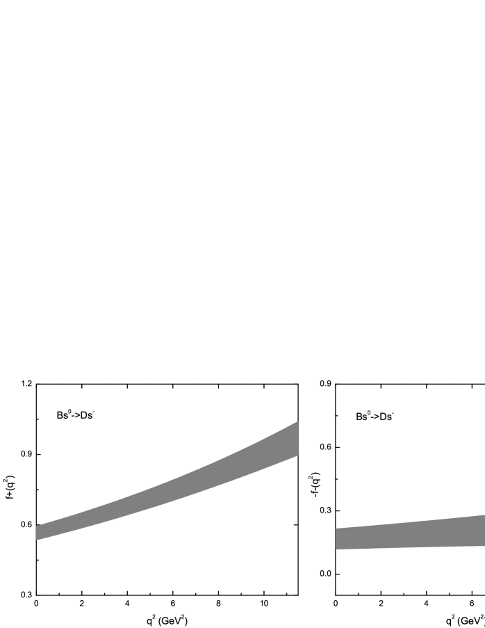
Figure 1: Form factors of $B^{0}_{s}\rightarrow D_{s}^{-}$ weak transition.

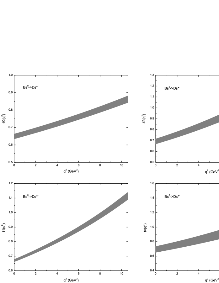
Figure 2: Form factors of $B^{0}_{s}\rightarrow D_{s}^{*-}$ weak transitions.

Table 1: Form factors of $B^{0}_{s}\rightarrow D_{s}^{-}$ and $B^{0}_{s}\rightarrow D_{s}^{*-}$ transitions at $q^{2}=0$ GeV².

	This work	BSW [9]	QCDSR [12]	LCSR [15]	CLFQM [14]
$f_{+}(0)$	$0.57^{+0.02}_{-0.03}$	0.61	$0.7\pm 0.1$	0.43
$f_{-}(0)$	$-0.17^{+0.05}_{-0.04}$			$-0.17$
$f_{V}(0)$	$0.70^{+0.03}_{-0.04}$	0.64	$0.63\pm 0.05$		$0.74\pm 0.05$
$f_{0}(0)$	$-0.65^{+0.01}_{-0.01}$	$-0.56$	$-0.62\pm 0.01$		$-0.61\pm 0.03$
$f_{1}(0)$	$0.67^{+0.01}_{-0.01}$	0.59	$0.75\pm 0.07$		$0.59\pm 0.04$
$f_{2}(0)$	$-0.70^{+0.03}_{-0.01}$

For semi-leptonic $B_{s}^{0}\rightarrow D_{s}^{(*)-}l^{+}\nu_{l}$ decays induced by $\bar{b}\rightarrow\bar{c}\nu_{l}\bar{l}$ transition, the effective Hamiltonian can be written as [15]

$$\mathcal{H}_{\mathrm{eff}}=\frac{G_{F}}{\sqrt{2}}V^{*}_{cb}\bar{b}\gamma_{\mu}(1-\gamma_{5})c\bar{\nu}_{l}\gamma^{\mu}(1-\gamma_{5})l.$$ (36)

The amplitude of $B_{s}^{0}\rightarrow D_{s}^{(*)-}l^{+}\nu_{l}$ decays could be obtained by sandwiching equation (36) between the initial and final states, which reads

$$\mathcal{M}=\frac{G_{F}}{\sqrt{2}}V^{*}_{cb}\bar{\nu}_{l}\gamma^{\mu}(1-\gamma_{5})l\langle D^{(*)-}_{s}|\bar{b}\gamma_{\mu}(1-\gamma_{5})c|B_{s}^{0}\rangle.$$ (37)

The width of a semi-leptonic decay is $\Gamma=\frac{1}{8M_{B_{s}}(2\pi)^{3}}\int\sum_{\mathrm{pol}}|\mathcal{M}|^{2}dE_{l}dE_{f}$ where $E_{l}$ and $E_{f}$ are the energies of the lepton and the meson in the final state respectively. With the form factors calculated, we estimate the branching ratios of semi-leptonic $B_{s}^{0}\rightarrow D_{s}^{(*)-}l^{+}\nu_{l}$ decays. The results are listed in Table 2 together with those from other approaches. The orders of magnitude for those branching ratios are consistent with each other. The $B_{s}^{0}\rightarrow D_{s}^{(*)-}e^{+}\nu_{e}$ decay rates have been studied in the same model in  [40] as used here. But the parameters and the formulation of the transition matrix elements used in that reference are different from those in this work, thus their results are larger. The parameters used in calculation such as $V_{cb}$, $\tau_{B_{s}^{0}}$ are shown in the next subsection.

Table 2: Branching ratios for semi-leptonic $B_{s}^{0}\rightarrow D_{s}^{(*)-}l^{+}\nu_{l}$ decays compared with those from other approaches.

Processes	This work	CQM [24]	QCDSR [13]	LCSR [15]	CLFQM [14]
$B_{s}^{0}\rightarrow D_{s}^{-}l^{+}\nu_{l}~{}(l=e,\mu)$	$(1.4-1.7)~{}\%$	$(2.73-3.00)\%$	$(2.8-3.8)\%$	$1.0^{+0.4}_{-0.3}~{}\%$
$B_{s}^{0}\rightarrow D_{s}^{-}\tau^{+}\nu_{\tau}$	$(4.7-5.5)\times 10^{-3}$			$3.3^{+1.4}_{-1.1}\times 10^{-3}$
$B_{s}^{0}\rightarrow D_{s}^{*-}l^{+}\nu_{l}~{}(l=e,\mu)$	$(5.1-5.8)~{}\%$	$(7.49-7.66)\%$	$(1.89-6.61)\%$		$5.2^{+0.6}_{-0.6}~{}\%$
$B_{s}^{0}\rightarrow D_{s}^{*-}\tau^{+}\nu_{\tau}$	$(1.2-1.3)~{}\%$				$1.3^{+0.2}_{-0.1}~{}\%$

4.2 Non-leptonic $B_{s}$ decay

Now we can use the form factors to estimate the decay rates of $B_{s}^{0}$. The CKM matrix elements used in our calculation are [25]

$$\begin{array}[]{ccc}|V_{ud}|=0.97425,&|V_{us}|=0.2252,&|V_{ub}|=3.89\times 10^{-3},\\ |V_{cd}|=0.230,&|V_{cs}|=0.9735,&|V_{cb}|=0.0406.\end{array}$$

The lifetime $\tau_{B_{s}^{0}}=1.472\times 10^{-12}s$ [25] is taken in calculation. The Wilson coefficients are quoted from [41], and for $\mu\sim m_{b}$, they are:

$$\begin{array}[]{ccccc}C_{1}=1.0849,&C_{2}=-0.1902,&C_{3}=0.0148,&C_{4}=-0.0362,&C_{5}=0.0088,\\ C_{6}=-0.0422,&\frac{C_{7}}{\alpha_{e}}=-0.0007,&\frac{C_{8}}{\alpha_{e}}=0.0565,&\frac{C_{9}}{\alpha_{e}}=-1.3039,&\frac{C_{10}}{\alpha_{e}}=0.2700,\\ \end{array}$$

where $\alpha_{e}(M_{W})=1/128$ is the electromagnetic coupling constant. The strong coupling constant is taken as $\alpha_{s}(m_{b})=0.216$. The decay constants used in this paper are shown in Table 3. Other inputs in pQCD analysis such as the wave functions and the Jet function appearing in the non-factorizable amplitudes and annihilation amplitudes are taken as the same as in [22].

Table 3: Decay constants used in our calculation in unit of MeV.

$f_{\pi}$	$f_{k}$	$f_{D}$	$f_{D_{s}}$	$f_{\rho}$	$f_{k^{*}}$	$f_{a_{1}}$
130 [25]	156 [25]	$207^{+9}_{-9}$ [25]	$258^{+6}_{-6}$ [25]	$205^{+9}_{-9}$ [42]	$217^{+5}_{-5}$ [42]	229 [43]
$f_{D^{*}}$	$f_{D_{s}^{*}}$	$f_{D^{*}_{0}}$	$f_{D_{s0}^{*}}$	$f_{D_{s1}(2460)}$	$f_{D_{s1}(2536)}$	$f_{B_{s}}$
$245^{+20}_{-20}$ [44]	$272^{+16}_{-16}$[44]	$137^{+4}_{-5}~{}\cite[cite]{[\@@bibref{}{Fu}{}{}]}$	$109^{+4}_{-5}~{}\cite[cite]{[\@@bibref{}{Fu}{}{}]}$	$227^{+22}_{-19}~{}\cite[cite]{[\@@bibref{}{Fu}{}{}]}$	$77.3^{+12.4}_{-9.8}~{}\cite[cite]{[\@@bibref{}{Fu}{}{}]}$	0.23 [22]

With these input parameters, we calculate the branching ratios of non-leptonic $\bar{B}_{s}^{0}$ to charmed particle decays. The results are listed in Table 4, together with those from other methods, as well as with available experimental data. The branching ratios of double charmed decays shown in the table are the CP averaged values: $\frac{1}{2}(\mathcal{B}(B_{s}^{0}\rightarrow f)+\mathcal{B}(\bar{B}_{s}^{0}\rightarrow\bar{f}))$, where $\mathcal{B}$ denotes branching ratio. The momentum transfer of $\bar{B}^{0}_{s}\rightarrow D_{s}^{(*)+}L^{-}$ decays, where $L^{-}$ is a light meson, is $q^{2}\sim 0-1.5~{}\mathrm{GeV}^{2}$, and the momentum transfer of the double charmed decays is $q^{2}\sim 3.5-6.4~{}\mathrm{GeV}^{2}$.

Table 4: The (averaged) branching ratios of $\bar{B}^{0}_{s}\rightarrow D_{s}^{(*)+}X^{-}$ in the unit of $\%$. Our results with pQCD represent those with non-factorziable and annihilation contributions estimated in the pQCD approach. The parameters in [10, 12, 46] are replaced by the ones used in our paper: $|V_{cb}|=0.04$, $\tau_{B_{s}^{0}}=1.472\times 10^{-12}$s, $a_{1}=1.02$. The results of $\bar{B}^{0}_{s}\rightarrow D^{+}_{s}X^{-}$ in the 7th column are quoted from [15] and the results of $\bar{B}^{0}_{s}\rightarrow D^{*+}_{s}X^{-}$ in the 7th column are quoted from [14]. Experimental data are quoted from [25, 26].

channels	Ours (FA)	Ours (pQCD)	BSW [10]	QCDSR [12]	HQET [46]	[14] [15]	pQCD [22]	Experimental Data
$D_{s}^{+}\pi^{-}$	$0.27^{+0.02}_{-0.03}$	$0.27^{+0.02}_{-0.03}$	0.37	0.41	0.31	$0.17^{+0.07}_{-0.06}$	$0.196^{+0.106}_{-0.075}$	$0.32\pm 0.05$
$D_{s}^{+}\rho^{-}$	$0.64^{+0.12}_{-0.11}$	$0.60^{+0.11}_{-0.11}$	0.94	1.1	0.82	$0.42^{+0.17}_{-0.14}$	$0.47^{+0.249}_{-0.177}$	$0.85^{+0.13}_{-0.12}\pm 0.11\pm 0.13$
$D_{s}^{+}k^{-}$	$0.021^{+0.002}_{-0.002}$	$0.021^{+0.001}_{-0.002}$	0.028	0.033	0.023	$0.013^{+0.005}_{-0.004}$	$0.0170^{+0.0087}_{-0.0066}$
$D_{s}^{+}k^{*-}$	$0.038^{+0.005}_{-0.005}$	$0.038^{+0.005}_{-0.005}$	0.049	0.049	0.040	$0.024^{+0.010}_{-0.008}$	$0.0281^{+0.0147}_{-0.0109}$
$D_{s}^{+}a_{1}^{-}$	$0.75^{+0.06}_{-0.08}$		0.88	0.9
$D_{s}^{*+}\pi^{-}$	$0.31^{+0.03}_{-0.02}$	$0.30^{+0.03}_{-0.03}$	0.28	0.16	0.31	$0.35^{+0.04}_{-0.04}$	$0.189^{+0.103}_{-0.072}$	$0.24^{+0.05}_{-0.04}\pm 0.03\pm 0.04$
$D_{s}^{*+}\rho^{-}$	$0.90^{+0.15}_{-0.15}$	$0.91^{+0.16}_{-0.15}$	0.88	1.1	0.97	$1.18^{+0.33}_{-0.31}$	$0.523^{+0.283}_{-0.195}$	$1.19^{+0.22}_{-0.20}\pm 0.17\pm 0.18$
$D_{s}^{*+}k^{-}$	$0.024^{+0.002}_{-0.002}$	$0.024^{+0.001}_{-0.003}$	0.020	0.016	0.023	$0.028^{+0.003}_{-0.003}$	$0.0164^{+0.0084}_{-0.0064}$
$D_{s}^{*+}k^{*-}$	$0.056^{+0.006}_{-0.007}$	$0.058^{+0.007}_{-0.007}$	0.048	0.049	0.053	$0.055^{+0.006}_{-0.006}$	$0.0322^{+0.0183}_{-0.0124}$
$D_{s}^{*+}a_{1}^{-}$	$1.3^{+0.1}_{-0.1}$		1.1
$D_{s}^{+}D^{-}$	$0.031^{+0.006}_{-0.005}$	$0.036_{-0.006}^{+0.007}$	0.027	0.041	0.049	$0.011^{+0.004}_{-0.004}$	$0.022^{+0.014}_{-0.010}$
$D_{s}^{+}D^{*-}$	$0.034^{+0.009}_{-0.008}$	$0.041^{+0.011}_{-0.011}$	0.031	0.033	0.034	$0.014^{+0.006}_{-0.005}$	$0.021^{+0.013}_{-0.009}$
$D_{s}^{+}D_{0}^{*-}$	$0.012^{+0.002}_{-0.002}$					$0.002^{+0.001}_{-0.001}$
$D_{s}^{*+}D^{-}$	$0.032^{+0.006}_{-0.006}$	$0.038^{+0.006}_{-0.008}$	0.013	0.016	0.036	$0.037^{+0.004}_{-0.004}$	$0.027^{+0.017}_{-0.011}$
$D_{s}^{*+}D^{*-}$	$0.11^{+0.02}_{-0.03}$	$0.13^{+0.03}_{-0.03}$	0.074	0.065	0.11	$0.086^{+0.010}_{-0.009}$	$0.039^{+0.026}_{-0.019}$
$D_{s}^{*+}D_{0}^{*-}$	$0.010^{+0.002}_{-0.001}$
$D_{s}^{+}D_{s}^{-}$	$0.83^{+0.10}_{-0.10}$	$1.3^{+0.1}_{-0.3}$	0.51	0.82	1.2	$0.35^{+0.14}_{-0.12}$	$0.55^{+0.36}_{-0.24}$	$1.04\pm 0.35$
$D_{s}^{+}D_{s}^{*-}$	$0.70^{+0.16}_{-0.15}$	$1.0^{+0.2}_{-0.2}$	0.57	0.65	0.77	$0.33^{+0.13}_{-0.11}$	$0.48^{+0.31}_{-0.21}$
$D_{s}^{*+}D_{s}^{-}$	$0.84^{+0.12}_{-0.12}$	$1.2^{+0.2}_{-0.1}$	0.23	0.33	0.81	$0.92^{+0.11}_{-0.11}$	$0.70^{+0.44}_{-0.31}$	$2.75^{+0.83}_{-0.71}\pm 0.69$
$D_{s}^{*+}D_{s}^{*-}$	$2.4^{+0.4}_{-0.4}$	$3.0^{+0.5}_{-0.5}$	1.48	1.3	3.2	$2.36^{+0.40}_{-0.38}$	$0.99^{+0.72}_{-0.54}$	$3.08^{+1.22+0.85}_{-1.04-0.86}$
$D_{s}^{+}D_{s0}^{*-}$	$0.13^{+0.01}_{-0.02}$					$0.053^{+0.022}_{-0.018}$
$D_{s}^{+}D_{s1}^{-}(2460)$	$0.37^{+0.12}_{-0.10}$
$D_{s}^{+}D_{s1}^{-}(2536)$	$0.039^{+0.019}_{-0.013}$
$D_{s}^{*+}D_{s0}^{*-}$	$0.12^{+0.02}_{-0.02}$
$D_{s}^{*+}D_{s1}^{-}(2460)$	$1.8^{+0.4}_{-0.4}$
$D_{s}^{*+}D_{s1}^{-}(2536)$	$0.21^{+0.08}_{-0.06}$

Compared our FA results and the results with corrections estimated by the pQCD approach (we will call them the pQCD corrected results), it can be found that the non-factorizable effects (and annihilation contributions when exist) for $\bar{B}^{0}_{s}\rightarrow D^{(*)+}_{s}+L^{-}$ channels make little corrections to the FA results. For double charmed $B_{s}$ decays, the factorizable color-favored diagrams still dominate the decay widths, but contributions from other diagrams give up to $\sim 20\%$ corrections. We also estimate some $\bar{B}^{0}_{s}\rightarrow D^{(*)}_{s}+S(A)$ decay rates under the FA, where $S$ represents scalar and $A$ stands for axial vector, but the uncertainties due to non-factorizable effects should be realized. The results in the 2, 4-7 columns are calculated in the FA, but with different approaches to evaluate form factors. For $\bar{B}^{0}_{s}\rightarrow D_{s}^{+}X^{-}$ decays, the results from the FA are roughly consistent with each other except the values from light cone sum rules (LCSR) approach, which are smaller than others. This discrepancy reflects the difference of form factors, which has been shown explicitly in Table 1. For $\bar{B}^{0}_{s}\rightarrow D_{s}^{*+}X^{-}$ decays, our results are consistent with HQET and CLFQM values, but larger than those in BSW and QCDSR methods.

Now we turn to compare the our results with the pQCD results in [22]. The major difference between our pQCD corrected results and their fully pQCD results is that, for calculating factorizable color-favored contributions, we estimate them in terms of our form factors, while in [22] all the contributions are calculated in the pQCD approach. Besides, some input parameters are different between the two works. The comparison can be seen from Table 4: most of the pQCD results are smaller than our FA results as well as the pQCD corrected results, but close to LCSR results. The Isgur-Wise form factor at maximum recoil in the pQCD is $\xi^{B_{s}\rightarrow D_{s}}_{+}=0.44$, whereas the corresponding quantity in our work is $\xi_{+}=(M_{B_{s}}(f_{+}+f_{-})+M_{D_{s}}(f_{+}-f_{-}))/2\sqrt{M_{B_{s}}M_{D_{s}}}=0.55$. Besides, authors of [22] found that the form factors from their pQCD calculations are similar with those from LCSR. Therefore, we can simply state that form factors from the pQCD approach in [22] are smaller than ours, which means that the discrepancies in decay rates between their pQCD results and ours could be attributed to the difference in form factors, rather than non-factorizable effects.

Thanks to the efforts done by Belle, CDF, D0 and other Collaborations, some experimental data of two-body non-leptonic $B_{s}$ decays are available now. We can see from Table 4 that our results agree well with the present experimental data. Since only some $\bar{B}^{0}_{s}\rightarrow D_{s}^{(*)+}X^{-}$ decay modes have been observed and the experimental errors are still large till now, it is expected in the near future more precise tests could be made on theoretical predictions as the increase of the $B_{s}^{0}$ events.

We now investigate the direct CP asymmetries of $B_{s}\rightarrow D_{s}^{(*)}D_{q}^{(*)}$ decays. The results together with $D_{1}$, $D_{2}$ are shown in Table 5. $D_{1}$, $D_{2}$ are defined in equation (32). Their values with the weak phase $\gamma$ determine the direct CP asymmetries. We show both the CPAs estimated under FA and in the pQCD approach. The discrepancy between FA and pQCD (or our pQCD corrected results) is obvious and is found mainly arising from the strong phases. It should be mentioned that another method called QCD improved factorization, which can cover the non-factorizable effects as well as pQCD, makes quite different predictions on CP asymmetries of some decay modes compared to pQCD. The reason is that the leading sources of the strong phase are different between the two approaches [47]. According to our results in Table 5, most of the direct CP asymmetries are too small to be tested experimentally for now.

Table 5: The direct CP asymmetries in double charmed non-leptonic decays of $\bar{B}_{s}^{0}$ in the unit of $10^{-2}$. $D_{1}$ and $D_{2}$ are defined as $\mathcal{A}_{CP}^{\mathrm{dir}}\equiv D_{1}\frac{\sin\gamma}{1+D_{2}\cos\gamma}$, where $\gamma$ is the weak phase (see equations (31,32)). In calculation, the weak phase is taken as $\gamma=68.8^{\circ}$. We show the results with non-factorziable and annihilation contributions estimated in the pQCD approach. The FA results are also shown in the brackets.

Final States	$D_{1}$ in this work		$D_{2}$ in this work		$\mathcal{A}_{CP}^{\mathrm{dir}}$ in this work		$\mathcal{A}_{CP}^{\mathrm{dir}}$ in [22]
$D_{s}^{+}D^{-}$	$-0.36\sim-0.24$	(5.3)	$9.8$	(10)	$-0.3\sim-0.2$	(4.8)	$-0.5_{-0.1-0.2}^{+0.0+0.1}$
$D_{s}^{+}D_{s}^{-}$	$0.12\sim 0.15$	(-0.32)	-0.47	(-0.97)	$0.1$	(-0.30)
$D_{s}^{+}D^{*-}$	$-0.064\sim 0.039$	(1.5)	3.1	(2.6)	$-0.06\sim 0.04$	(1.4)	$-0.1_{-0.0-0.0}^{+0.1+0.0}$
$D_{s}^{+}D_{s}^{*-}$	$0.048\sim 0.063$	($-0.081$)	-0.16	(-0.14)	$0.05\sim 0.06$	($-0.076$)
$D_{s}^{*+}D^{-}$	$0.56\sim 0.71$	(-0.46)	-0.69	(-1.6)	$0.5\sim 0.7$	(-0.43)	$0.4_{-0.0-0.1}^{+0.0+0.1}$
$D_{s}^{*+}D_{s}^{-}$	$-0.074\sim-0.064$	($0.027$)	$0.032$	(0.13)	$-0.07\sim-0.06$	($0.025$)
$D_{s}^{*+}D^{*-}$	$0.\sim 0.13$	(1.5)	2.9	(2.6)	$0.\sim 0.1$	(1.4)	$-0.1_{-0.1-0.1}^{+0.0+0.0}$
$D_{s}^{*+}D_{s}^{*-}$	$-0.0018\sim 0.015$	($-0.081$)	-0.20	(-0.14)	$-0.002\sim 0.01$	($-0.076$)

The results of polarization fractions of $B_{s}^{0}\rightarrow VV(A)$ decays are listed in Table 6, compared with other theoretical estimates and available experimental data. From the table, we can say that the non-factorizable contributions (and annihilation contributions when exit) do not give sufficient corrections on factorizations. Besides, it could be found that although our form factors are different from those in [22], the polariztions are still similar, which tells that the polariztions are less affceted by the form factors. Please note that for decays with a $D_{s}^{*}$ and a light meson in the final state, $R_{L}\sim 0.8\gg R_{\parallel},~{}R_{\perp}$; for decays with two charmed mesons in the final state, $R_{L}\sim R_{\parallel}\sim 0.5\gg R_{\perp}$. The similar results have been found in $B\rightarrow VV$ decays.

Table 6: Polarization fractions of $\bar{B}_{s}^{0}\rightarrow VV$ or $VA$ decays. $R_{L}$, $R_{\parallel}$ and $R_{\perp}$ are longitudinal, transverse parallel and transverse perpendicular polarization fractions, respectively. Our results with pQCD represent those with non-factorziable and annihilation contributions estimated in the pQCD approach.

Final States		Ours (FA)	Ours (pQCD)	[22]	Experiment [26]
$D_{s}^{*+}\rho^{-}$	$R_{L}$	$0.874^{+0.004}_{-0.003}$	$0.854^{+0.004}_{-0.005}$	0.87	$1.05^{+0.08}_{-0.10}(\mathrm{stat})^{+0.03}_{-0.04}(\mathrm{syst})$
	$R_{\parallel}$	$0.104^{+0.005}_{-0.004}$	$0.113^{+0.005}_{-0.005}$
$D_{s}^{*+}K^{*-}$	$R_{L}$	$0.841^{+0.004}_{-0.005}$	$0.857^{+0.003}_{-0.003}$	0.83
	$R_{\parallel}$	$0.133^{+0.005}_{-0.006}$	$0.104^{+0.004}_{-0.004}$
$D_{s}^{*+}a_{1}^{-}$	$R_{L}$	$0.738^{+0.005}_{-0.007}$
	$R_{\parallel}$	$0.221^{+0.007}_{-0.008}$
$D_{s}^{*+}D^{*-}$	$R_{L}$	$0.525^{+0.006}_{-0.006}$	$0.511^{+0.010}_{-0.006}$	$0.56\pm 0.14$
	$R_{\parallel}$	$0.416^{+0.009}_{-0.009}$	$0.439^{+0.009}_{-0.010}$
$D_{s}^{*+}D_{s}^{*-}$	$R_{L}$	$0.503^{+0.005}_{-0.006}$	$0.537^{+0.006}_{-0.004}$	$0.53\pm 0.15$
	$R_{\parallel}$	$0.439^{+0.009}_{-0.010}$	$0.427^{+0.006}_{-0.012}$
$D_{s}^{*+}D_{s1}^{-}(2460)$	$R_{L}$	$0.436^{+0.004}_{-0.004}$
	$R_{\parallel}$	$0.512^{+0.008}_{-0.008}$
$D_{s}^{*+}D_{s1}^{-}(2536)$	$R_{L}$	$0.424^{+0.003}_{-0.004}$
	$R_{\parallel}$	$0.527^{+0.008}_{-0.007}$

To conclude, we note that the form factors of $B_{s}^{0}\rightarrow D_{s}^{-}$ and $B_{s}^{0}\rightarrow D_{s}^{*-}$ estimated in this work are roughly consistent with other theoretical estimates such as the QCD sum rule, the light-front quark model and so on. Using the derived form factors, branching ratios of semi-leptonic and non-leptonic $B^{0}_{s}$ decays to charmed particles are estimated. For non-leptonic decays we evaluate amplitudes under the factorization approximation as well as in the pQCD approach (for non-factorizable and annihilation contributions). Our predictions on decay rates are found to agree well with the available experimental data. Direct CP asymmetries estimated in FA and in pQCD are quite different (even have different sign). Generally, the CPAs of $\bar{B}_{s}^{0}\rightarrow D_{s}^{(*)+}D_{q}^{-}$ are less than $1\%$. Polarization fractions of $B_{s}\rightarrow D_{s}^{*}V(A)$ decays follow the similar rule as $B\rightarrow VV$ decays, that is, for decays with a $D_{s}^{*}$ and a light meson in the final state, $R_{L}\sim 0.8\gg R_{\parallel},~{}R_{\perp}$, for decays with two charmed mesons in the final state, $R_{L}\sim R_{\parallel}\sim 0.5\gg R_{\perp}$.

References

- [1] D.-S. Du and Z.-Z. Xing, Phys. Rev. D 48, (1993) 3400; D.-S. Du and M.-Z. Yang, Phys. Lett. B 358, (1995) 123; B. Tseng, Phys. Lett. B 446, (1999) 125; Y.-H. Chen, H.-Y. Cheng and B. Tseng, Phys. Rev. D 59, (1999) 074003; C.-H. Chen, Phys. Lett. B 520, (2001) 33; J.-F. Sun, G.-H. Zhu and D.-S. Du, Phys. Rev. D 68, (2003) 054003; X.-Q. Li, G.-R. Lu and Y.-D. Yang, Phys. Rev. D 68, (2003) 114015; A. R. Williamson and J. Zupan, Phys. Rev. D 74, (2006) 014003; Z.-J. Xiao, X.-F. Chen and D.-Q. Guo, Eur. Phys. J. C 50, (2007) 363; A. Ali, et al, Phys. Rev. D 76, (2007) 074018; M. Beneke, J. Rohrer and D. Yang, Nucl. Phys. B 774, (2007) 64; H.-Y. Cheng and C-K. Chua, Phys. Rev. D 80, (2009) 114026.
- [2] R. Aleksan, A. Le Yaouanc, L. Oliver, O. Pne and J. C. Raynal, Phys. Lett. B 316, (1993) 567.
- [3] A. Dighe, I. Dunietz and R. Fleischer, Eur. Phys. J. C 6, (1999) 647.
- [4] R. Fleischer, Nucl. Phys. B 671, (2003) 459; Eur. Phys. J. C 51, (2007) 849.
- [5] Z.-Z. Xing, Phys. Lett. B 443, (1998) 365.
- [6] P. Ball and R. Fleischer, Phys. Lett. B 475, (2000) 111.
- [7] I. Dunietz, R. Fleischer and U. Nierste, Phys. Rev. D 63, (2001) 114015.
- [8] C. S. Kim, R.-M. Wang and Y.-D. Yang, Phys. Rev. D 79, (2009) 055004.
- [9] G. Kramer and W. F. Palmer, Phys. Rev. D 46, (1992) 3197; M. Wirbel, Prog. Part. Nucl. Phys., 21, (1988) 33.
- [10] J. Bijnens and F. Hoogeveen, Phys. Lett. B 283, (1992) 434.
- [11] M. Wirbel, B. Stech, and M. Bauer, Z. Phys. C 29, (1985) 637; M. Bauer, B. Stech, and M. Wirbel, Z. Phys. C 34, (1987) 103.
- [12] P. Blasi, P. Colangelo, G. Nardulli and N. Paver, Phys. Rev. D 49, (1994) 238.
- [13] K. Azizi, R. Khosravi and F. Falahati, Int. J. Mod. Phys. A 24, (2009) 5845; K. Azizi, Nucl. Phys. B 801, (2008) 70; K. Azizi and M. Bayar, Phys. Rev. D 78, (2008) 054011.
- [14] G. Li, F.-L. Shao and W. Wang, Phys. Rev. D 82, (2010) 094031.
- [15] R.-H. Li, C.-D. L and Y-M. Wang, Phys. Rev. D 80, (2009) 014005.
- [16] E. E. Salpeter, H. A. Bethe, Phys. Rev. 84, (1951) 1232; E. E. Salpeter, Phys. Rev. 87, (1952) 328.
- [17] S. Mandelstam, Proc. R. Soc. London 233 (1955) 248.
- [18] A. Ali, G. Kramer, and C.-D. L, Phys. Rev. D 58, (1998) 094009; H.-Y. Cheng and K.-C. Yang, Phys. Rev. D 62, (2000) 054029.
- [19] Y.Y. Keum, H.-N. Li, and A. I. Sanda, Phys. Lett. B 504 (2001) 6 ; Phys. Rev. D 63 (2001) 054008.
- [20] M. Beneke. G. Buchalla, M. Neubert and C. T. Sachrajda, Phys. Rev. Lett. 83 (1999) 1914; Nucl. Phys. B 591 (2000) 313.
- [21] C.W. Bauer, S. Fleming, D. Pirjol, and I.W. Stewart, Phys. Rev. D 63 114020 (2001).
- [22] R.-H. Li, C.-D. L, and H. Zou, Phys. Rev. D 78, (2008) 014018; R.-H. Li, C.-D. L, A. I. Sanda, and X-X. Wang, Phys. Rev. D 81, (2010) 034006.
- [23] R. Ferrandes, Talk given at IFAE 2006, Pavia, April 19-21 (2006), Report No. BARI-TH/06-543.
- [24] S.-M. Zhao, X. Liu and S.-J. Li, Eur. Phys. J. C 51, (2007) 601.
- [25] K. Nakamura et al. (Particle Data Group), J. Phys. G 37, (2010) 075021.
- [26] R. Louvot et al. (Belle Collaboration), Phys. Rev. Lett. 104, (2010) 231801; S. Esen et al. (Belle Collaboration), Phys. Rev. Lett. 105, (2010) 201802.
- [27] C.-H. Chang and J.-K. Chen, Commun. Theor. Phys. 44, (2005) 646; C.-H. Chang, J.-K. Chen, X.-Q. Li and G.-L. Wang, Commun. Theor. Phys. 43, (2005) 113.
- [28] C.-H. Chang, G.-L. Wang, Sci. China G 53, (2010) 2005.
- [29] C. S. Kim, G.-L. Wang, Phys. Lett. B 584, (2004) 285; G.-L. Wang, Phys. Lett. B 633, (2006) 492;
- [30] C.-H. Chang and Y.-Q. Chen, Commun. Theor. Phys. 23 (1995) 451.
- [31] C.-H. Chang, J.-K. Chen and G.-L. Wang, Commun. Theor. Phys. 46, (2006) 467.
- [32] Z.-h. Wang, G.-L. Wang and C.-H. Chang, J. Phys. G 39, (2012) 015009.
- [33] A. Bender, C. D. Roberts and L. V. Smekal, Phys. Lett. B 380, (1996) 7; P. Maris, A. Raya, C. D. Roberts and S. M. Schmidt, Eur. Phys. J. A 18, (2003) 231;P. Maris and C. D. Roberts, Int. J. Mod. Phys. E 12, (2003) 297.
- [34] M. A. Ivanov, Yu. L. Kalinovsky and C. D. Roberts, Phys. Rev. D 60, (1999) 034018; M. A. Ivanov, J. G. Krner, S. G. Kovalenko and C. D. Roberts, Phys. Rev. D 76, (2007) 034018; B. El-Bennich, M. A. Ivanov and C. D. Roberts. Phys. Rev. C 83, (2011) 025205.
- [35] T. Nguyen, N. A. Souchlas and P. C. Tandy. AIP Conf. Proc. 1116, (2009) 327.
- [36] G. Buchalla, A. J. Buras and M. E. Lautenbacher, Rev. Mod. Phys. 68, (1996) 1125; A. J. Buras, hep-ph/9806471, (1998).
- [37] Y.-S. Dai and D.-S. Du. Eur. Phys. J. C 9, (1999) 557.
- [38] C.-H. Chen, C.-Q. Geng and Z.-T. Wei, Eur. Phys. J. C 46, (2006) 367.
- [39] C.-F. Qiao, H.-W. Huang and K.-T. Chao, Phys. Rev. D 54, (1996) 2273; Phys. Rev. D 60, (1999) 094004.
- [40] J.-M. Zhang and G.-L. Wang, Chin. Phys. Lett. 27, (2010) 051301.
- [41] J.-F. Sun, Y.-L. Yang, W.-J. Du and H.-L. Ma, Phys. Rev. D 77, (2008) 114004.
- [42] P. Ball and R. Zwicky, Phys. Rev. D 71, (2005) 014029.
- [43] Z. Luo and J. L. Rosner, Phys. Rev. D 64, (2001) 094001.
- [44] D. Becirevic et al. Phys. Rev. D 60, (1999) 074501.
- [45] H.-F. Fu, Y. Jiang, C. S. Kim and G.-L. Wang, J. High Energy Phys. 06 (2011) 015.
- [46] A. Deandrea, N. Di Bartolomeo, R. Gatto and G. Nardulli, Phys. Lett. B 318, (1993) 549.
- [47] H.-N. Li, Prog. Part. Nucl. Phys. 51, (2003) 85.