KUNS-2344 RIKEN-MP-23
D term and gaugino masses
in gauge mediation

Abstract

We systematically study supersymmetry breaking with non-vanishing F and D terms. We classify the models into two categories and find that a certain class of models necessarily has runaway behavior of scalar potential, while the other needs the Fayet-Iliopoulos term to break supersymmetry. The latter class is useful to have a simple model of gauge mediation where the vacuum is stable everywhere and the gaugino mass is generated at the one-loop order.

1 Introduction

Supersymmetric extension of the standard model is one of interesting and promising candidates for physics above the weak scale. Even if supersymmetry (SUSY) is realized at high-energy regime, it must be broken below the weak scale, because the superpartners of the standard model particles have not been observed. It is well known that SUSY breaking inside our visible sector often leads to phenomenological problems, for which one usually needs to introduce the hidden sector for SUSY breaking and its mediation.

Recently, several important properties of SUSY breaking were clarified in the framework of global SUSY with the canonical Kähler potential; the SUSY-breaking vacuum of F-term scalar potential has pseudo-moduli or tachyonic direction at tree level. In addition, a superpartner of a massless fermion remains massless or becomes tachyonic (even) when SUSY is broken in renormalizable Wess-Zumino models. The latter fact is called the Komargodski-Shih (KS) lemma in this paper. The general proof of these properties has recently been given in [1, 2, 3].

The above result has important phenomenological implications, particularly to the gauge mediation of SUSY breaking. The gauge mediation is one of interesting mechanisms to mediate SUSY breaking in the hidden sector to the visible sector at quantum level (for a review, see [4]). The presence of pseudo-moduli and the KS lemma imply vanishing gaugino masses at the one-loop order or the existence of tachyonic direction [3]. That is phenomenologically unfavorable since gaugino masses are relatively light compared with SUSY-breaking scalar masses. Such a problem was found empirically in a direct gauge mediation model [5] and a solution has been proposed with higher-energy local minimum [6].

It is natural to expect that the result would not hold if one changes any of the model assumptions, that is, the tree-level F-term scalar potential of global SUSY Wess-Zumino model with the canonical Kähler form. A possible remedy is to consider the effect of non-canonical (higher-dimensional) Kähler potential [7] such as in supergravity. This change however might spoil the predictability/calculability of gauge mediation. As for the loop-level effect, it would be interesting to combine the gauge mediation with the anomaly mediation [8] without losing their merits (see e.g. [9]).

Another interesting way out is to include the non-vanishing D-term scalar potential of additional gauge group. In this paper, we systematically study the SUSY breaking with F and D-term scalar potentials of global SUSY models in which the Kähler form is canonical. The models are classified into two categories under the criterion that the F-flatness conditions have a solution or not. We then call models are in the first class when there exists no solution, i.e. F-term SUSY breaking. On the other hand, we call models are in the second class when there exists a solution satisfying all the F-flatness conditions but it is destabilized by the D-term contribution. A non-vanishing (charged) F term is generally required to have a non-vanishing D term, and therefore SUSY-breaking models with F and D terms belong to each of these two classes.

In the first class, the pseudo-moduli appear in the F-term scalar potential. As we will show, once the D-term contribution is included, such a pseudo-moduli direction has a runaway behavior, where the expectation value runs away to the infinity and the vacuum is undetermined. In the second class, SUSY breaking can be realized when and only when a non-vanishing Fayet-Iliopoulos (FI) term is introduced. We thus find that the second class of models is useful to avoid the discussion of Komargodski and Shih and to generate one-loop order gaugino masses in the visible sector through gauge mediation.

This paper is organized as follows. In Section 2, we give a brief review on some important properties of SUSY-breaking models only with the F-term scalar potential. In Section 3, we systematically study generic aspects of F and D-term SUSY breaking. The above two classes of models are investigated in details. In Section 4, we present a simple model of gauge mediation and show that the gaugino mass is generated on the stable vacuum. Section 5 is devoted to summarizing our results. In Appendix, we summarize the stationary conditions for the first class of models discussed in Section 3.

2 F-term SUSY breaking

In this section, we briefly review some general features of F-term SUSY-breaking models, explaining the existence of a pseudo-moduli direction and the KS lemma as well as their implications to the gauge mediation.

2.1 Pseudo-moduli and the KS lemma

We consider a model with the following general renormalizable superpotential

$$W=\sum_{i}f_{i}\phi_{i}+\sum_{i,j}\frac{m_{ij}}{2}\phi_{i}\phi_{j}+\sum_{i,j,k}\frac{\lambda_{ijk}}{6}\phi_{i}\phi_{j}\phi_{k}\ ,$$ (2.1)

where $\phi_{i}$ are chiral superfields and the subscript $i$ denotes the species of them. The Kähler potential has the canonical form; $K=\sum_{i}|\phi_{i}|^{2}$. Then the scalar potential $V$ receives the F-term contribution and is written as

$$V=V_{F}=\sum_{i}\overline{W}_{\bar{i}}(\bar{\phi})W_{i}(\phi)\ ,$$ (2.2)

where $W_{i}$ represents the derivative of $W$ with respect to $\phi_{i}$. Here and hereafter we follow the conventional notation that chiral superfields and their lowest scalar components are denoted by the same letters.

Let us suppose that the model has a SUSY-breaking minimum at $\phi_{i}=\phi_{i}^{(0)}$ where at least one of the F components is non-vanishing,

$$W_{i}^{(0)}\equiv W_{i}(\phi^{(0)})\not=0\ ,$$ (2.3)

for some $i$. Throughout this paper, we use the superscript ⁽⁰⁾ to clarify that it is evaluated at the minimum of the F-term scalar potential, $\phi_{i}=\phi_{i}^{(0)}$. The minimum satisfies the stationary condition

$$V_{j}=\sum_{i}\overline{W}^{(0)}_{\bar{i}}W^{(0)}_{ij}=0\ .$$ (2.4)

Since $W^{(0)}_{ij}$ corresponds to the fermion mass matrix, the condition (2.4) implies that there is a massless fermion along the direction $\overline{W}_{\bar{i}}^{(0)}$ ($\not=0$). This is nothing but the massless Nambu-Goldstone fermion corresponding to SUSY breaking.

The boson mass-squared matrix at the minimum is given by

$$M_{B}^{2}=\begin{pmatrix}V_{\bar{i}j}&V_{\bar{i}\bar{j}}\\ V_{ij}&V_{i\bar{j}}\end{pmatrix}=\begin{pmatrix}\sum_{k}\overline{W}_{\bar{i}\bar{k}}^{(0)}W_{kj}^{(0)}&\sum_{k}\overline{W}^{(0)}_{\bar{i}\bar{j}\bar{k}}W^{(0)}_{k}\\[2.84526pt] \sum_{k}W^{(0)}_{ijk}\overline{W}^{(0)}_{\bar{k}}&\sum_{k}W_{ik}^{(0)}\overline{W}_{\bar{k}\bar{j}}^{(0)}\end{pmatrix},$$ (2.5)

in the basis $(\phi_{i},\bar{\phi}_{j})$. Consider a massless fermion denoted by the eigenvector $v_{i}$, that is, $W_{ij}^{(0)}v_{j}=0$. Along its superpartner direction $(v,\bar{v})$, the boson mass term in the scalar potential is evaluated as

$$\begin{pmatrix}v\\ \bar{v}\end{pmatrix}^{\!\dagger}\!M_{B}^{2}\begin{pmatrix}v\\ \bar{v}\end{pmatrix}=\sum_{i,j,k}v_{i}W^{(0)}_{ijk}\overline{W}^{(0)}_{\bar{k}}v_{j}+\text{c.c.}\ ,$$ (2.6)

which can be made negative by a phase rotation of the eigenvector $v$. Hence this must vanish,

$$\sum_{j,k}W^{(0)}_{ijk}\overline{W}^{(0)}_{\bar{k}}v_{j}=0\ ,$$ (2.7)

for a positive semi-definite Hermite $M_{B}^{2}$, that is, as long as the vacuum is stable. In other words, a superpartner of a massless fermion must be massless or tachyonic (even) when SUSY is broken [3]. In particular, Eq. (2.7) is explicitly written down for the massless Nambu-Goldstone fermion for SUSY breaking;

$$\sum_{j,k}W^{(0)}_{ijk}\overline{W}^{(0)}_{\bar{j}}\overline{W}^{(0)}_{\bar{k}}=0\ .$$ (2.8)

The F-term potential has a tree-level flat direction (pseudo-moduli) parametrized as

$$\phi_{i}=\phi^{(0)}_{i}+z\overline{W}_{\bar{i}}^{(0)}\ ,\quad z\in\mathbb{C}\ .$$ (2.9)

That is easily confirmed by showing that $W_{i}$ is invariant along this direction:

$$W_{i}\big{(}\phi^{(0)}+z\overline{W}^{(0)}\big{)}=W_{i}^{(0)}+z\sum_{j}W_{ij}^{(0)}\overline{W}_{\bar{j}}^{(0)}+\frac{1}{2}z^{2}\sum_{j,k}W_{ijk}^{(0)}\overline{W}_{\bar{j}}^{(0)}\overline{W}_{\bar{k}}^{(0)}=W_{i}^{(0)}\ ,$$ (2.10)

with the help of Eqs. (2.4) and (2.8).

We have discussed the KS lemma and the presence of pseudo-moduli for the SUSY-breaking Wess-Zumino models. These two properties hold even when a model contains higher-order superpotential terms such as in the generalized O’Raifeartaigh model discussed in [10]. The most generic superpotential form of generalized O’Raifeartaigh models studied in [3] is

$$W=\sum_{i=1}^{r}X_{i}f_{i}(\phi_{j})+g(\phi_{j})\ .$$ (2.11)

The numbers of $X_{i}$ and $\phi_{j}$ fields, $r$ and $s$ respectively, satisfy $r>s$, and $f_{i}(\phi)$ are generic functions of $\phi$. In this case, some F components in $X_{i}$ become nonzero in the SUSY-breaking vacuum, and the pseudo-moduli direction is therefore a linear combination of $X_{i}$. Many concrete examples of SUSY breaking is classified into this form and share the vacuum property discussed in this section.

2.2 Gaugino masses in gauge mediation

It was shown [3] that F-term SUSY-breaking models lead to a phenomenological problem when they are used for the hidden sector of gauge mediation; vanishing gaugino masses or unstable hidden sector somewhere in the pseudo-moduli space. To see this, let us start with the SUSY-breaking Wess-Zumino model in the canonical form

$$W=fX+\sum_{i,j}\frac{1}{2}(\lambda_{ij}X+m_{ij})\phi_{i}\phi_{j}+\sum_{i,j,k}\frac{1}{6}\lambda_{ijk}\phi_{i}\phi_{j}\phi_{k}\ .$$ (2.12)

The SUSY-breaking minimum satisfies $W_{X}\neq 0$ and the scalar potential has the corresponding pseudo-moduli direction. We assume for simplicity that $\det(\lambda X+m)$ is non-vanishing for generic $X$, that is, massless eigenstates are irrelevant for gauge mediation and removed from the following discussion. By definition, the determinant is a polynomial of $X$ and is expanded as

$$\det(\lambda X+m)=\sum_{n}c_{n}(\lambda,m)X^{n}\,.$$ (2.13)

Unless $c_{0}\neq 0$ and $c_{n}=0$ for $n>0$, one always finds a solution for $\det(\lambda X+m)=0$ at some point $X=X_{0}$ on the pseudo-moduli direction. This fact means that the mass matrix $(\lambda X_{0}+m)_{ij}$ has a zero eigenvalue and the corresponding eigenvector $v$ such that $(\lambda X_{0}+m)v=0$. Then the KS lemma, Eq. (2.7), is found to imply $\lambda v=mv=0$ if there is no tachyonic direction anywhere in the pseudo-moduli space. This contradicts with our assumption that $\det(\lambda X+m)$ is not identically zero. As a result, $\det(\lambda X+m)$ should not have any zero, and must be independent of $X$ ($c_{n}=0$ for $n>0$);

$$\det(\lambda X+m)=c_{0}=\text{const.}\ .$$ (2.14)

In gauge mediation, some fields $\phi_{M}$ play as the messenger of SUSY breaking which, by definition, have the gauge interaction to the standard model vector multiplets. The gauge invariance implies the mass matrix form

$$(\lambda_{ij}X+m_{ij})\phi_{i}\phi_{j}=\begin{pmatrix}\phi_{M}\\ \phi^{\prime}\end{pmatrix}^{T}\begin{pmatrix}(\lambda X+m)_{M}&0\\ 0&(\lambda X+m)^{\prime}\end{pmatrix}\begin{pmatrix}\phi_{M}\\ \phi^{\prime}\end{pmatrix}\ .$$ (2.15)

The above statement, Eq. (2.14), holds for each of sub-matrices, i.e.,

$$\det(\lambda X+m)_{M}={\rm const.}\ .$$ (2.16)

This fact leads to a problem that the standard-model gaugino masses are not generated at the leading order of gauge interactions;

$$M_{\tilde{g}}\propto\frac{\partial}{\partial X}\log\det(\lambda X+m)_{M}=0\ .$$ (2.17)

Thus the vacuum structure of F-term SUSY breaking has the phenomenological problem (or unstable vacuum) and is not suitable for gauge mediation. In the next section, we will examine how this situation is changed when the D-term scalar potential is included.

3 Including D-term potential

To circumvent the phenomenologically unfavorable result of F-term SUSY breaking, we examine in this section how the situation can change with the D-term potential included. For this purpose, we first present some useful relations between the F and D components, and then investigate the vacuum of SUSY-breaking models with F and D terms. Some discussions of the D-term potential in gauge mediation are given in [11].

3.1 Relations between F and D

Before proceeding the model classification, we give several useful relations between F and D components, satisfied identically and only on the vacuum.

In this paper we discuss the models with superpotential $W$ and U(1) gauge symmetry. The full scalar potential consists of the F and D terms

$$V=V_{F}+V_{D}\ ,$$ (3.1)

where the D-term contribution is explicitly given by

$$V_{D}=\frac{g^{2}}{2}D^{2},\qquad D=\sum_{i}q_{i}|\phi_{i}|^{2}\ .$$ (3.2)

Here $g$ denotes the gauge coupling constant and $q_{i}$ the U(1) charge of $\phi_{i}$. The U(1) gauge-invariant Lagrangian generally contains the linear term of vector superfield (the FI term [12]) with the coefficient $\xi$, and the D component is then modified as

$$D=\xi+\sum_{i}q_{i}|\phi_{i}|^{2}.$$ (3.3)

The formulas given below are valid in the presence of the FI term.

The U(1) transformation acts on $\phi_{i}$ as $\phi_{i}\to\phi_{i}+i\varepsilon q_{i}\phi_{i}$ where $\varepsilon$ is an infinitesimal parameter, and the U(1) gauge invariance of the (super)potential leads to

$$\sum_{i}W_{i}q_{i}\phi_{i}=0\ .$$ (3.4)

The field derivatives of this identity are also satisfied;

$$\sum_{i}W_{ij}q_{i}\phi_{i}+W_{j}q_{j}=0\ ,$$ (3.5)

$$\sum_{i}W_{ijk}q_{i}\phi_{i}+W_{jk}(q_{j}+q_{k})=0\ ,$$ (3.6)

where $j$ and $k$ are not summed over. They are rewritten by using the derivatives of the D component, $D_{\bar{i}}=q_{i}\phi_{i}$ and $D_{i\bar{j}}=q_{i}\delta_{ij}$, as

$$\sum_{i}W_{i}D_{\bar{i}}=0\ ,$$ (3.7)

$$\sum_{i}\big{(}W_{ij}D_{\bar{i}}+W_{i}D_{j\bar{i}}\big{)}=0\ ,$$ (3.8)

$$\sum_{i}\big{(}W_{ijk}D_{\bar{i}}+W_{ik}D_{j\bar{i}}+W_{ij}D_{k\bar{i}}\big{)}=0\ .$$ (3.9)

Other field identities can be obtained with various contractions, e.g.,

$$\sum_{i,j}W_{ij}D_{\bar{i}}\phi_{j}=0\ ,$$ (3.10)

$$\sum_{i}q_{i}|W_{i}|^{2}+\sum_{i,j}W_{ij}\overline{W}_{\bar{i}}D_{\bar{j}}=0\ ,$$ (3.11)

$$\sum_{i}q_{i}^{2}|W_{i}|^{2}-\sum_{i,j,k}D_{\bar{i}}W_{ij}\overline{W}_{\bar{j}\bar{k}}D_{k}=0\ .$$ (3.12)

On the vacuum, the stationary conditions impose additional constraints between F and D terms:

$$\sum_{i}W_{ij}\overline{W}_{\bar{i}}+g^{2}DD_{j}=0\ .$$ (3.13)

By multiplying $\overline{W}_{\bar{j}}$, $\phi_{j}$, $q_{j}\phi_{j}$ and taking the summation over $j$, we obtain

$$\sum_{i,j}W_{ij}\overline{W}_{\bar{i}}\overline{W}_{\bar{j}}=0\ ,$$ (3.14)

$$\sum_{i,j}\phi_{i}W_{ij}\overline{W}_{\bar{j}}+g^{2}D(D-\xi)=0\ ,$$ (3.15)

$$\sum_{i}q_{i}|W_{i}|^{2}-g^{2}D\sum_{i}|D_{i}|^{2}=0\ ,$$ (3.16)

where we have used the field identities given above. The last relation means an important fact that the D term gives a non-vanishing contribution to the scalar potential only if some F terms of U(1)-charged multiplets are non-vanishing. As seen below, this result is useful to classify and analyze the models with F and D terms.

3.2 Classification

The SUSY vacuum has the vanishing scalar potential, that is, all of F and D-flatness conditions are simultaneously satisfied.

F flatness : $$W_{i}=0 \quad(\text{for}\;{}^{\forall}i)\ ,$$ (3.17)

D flatness : $$D\,=\,0 \ .$$ (3.18)

Thus SUSY-breaking models with F and D terms are classified into two categories. We call a model is in the first class when there is no solution satisfying all the F-flatness conditions at the same time. The second class of models has a solution of the F-flatness conditions but that is destabilized by the D-term potential, which causes SUSY breaking. As mentioned above, the D-term effect appears only if $\sum_{i}q_{i}|W_{i}|^{2}$ is non-vanishing at the vacuum. Thus the above two classes are all possible situations leading to SUSY breaking.

For SUSY breaking, only F terms are effective in the first class of models, and the combination of F and D terms is important in the second class. We will study the first and second classes of models in the subsections 3.3 and 3.4, respectively. The results are summarized in Table 1. The third and fourth columns are our main results in this paper. The scalar potential in the first class of models turns out to have a runaway direction no matter whether the FI term is added or not, and thus this class cannot be applied to phenomenology as it stands. For the second class, SUSY is broken if a proper FI term is introduced, and it would be useful for model building such as gauge mediation.

	F-flatness	FI term	FI term
	solution	$\xi=0$	$\xi\neq 0$
First class	no	runaway	runaway
Second class	yes	SUSY	SUSY

Table 1: Classification of SUSY-breaking models with F and D terms.

3.3 The first class:  Runaway vacuum

3.3.1 Non-vanishing D term

The first class of models belong to the F-term SUSY breaking reviewed in the previous section. Therefore when only the F-term contribution is taken into account, the scalar potential has a pseudo-moduli direction. We first examine whether the situation is changed, i.e. the pseudo-moduli are uplifted once the D-term contribution is included. The (field-dependent) bosonic mass-squared matrix is given by

$$M_{B}^{2}=\begin{pmatrix}\sum_{k}\overline{W}_{\bar{i}\bar{k}}W_{kj}+g^{2}(D_{\bar{i}}D_{j}+DD_{\bar{i}j})&\sum_{k}\overline{W}_{\bar{i}\bar{j}\bar{k}}W_{k}+g^{2}D_{\bar{i}}D_{\bar{j}}\\[2.84526pt] \sum_{k}W_{ijk}\overline{W}_{\bar{k}}+g^{2}D_{i}D_{j}&\!\!\sum_{k}W_{ik}\overline{W}_{\bar{k}\bar{j}}+g^{2}(D_{i}D_{\bar{j}}+DD_{i\bar{j}})\end{pmatrix}\ .$$ (3.19)

If the minimum of the full scalar potential corresponds to $D=0$ and $W_{i}\neq 0$, the stationary condition (3.13) reduces to $\sum_{i}W_{ij}\overline{W}_{\bar{i}}=0$. Along the massless direction $\overline{W}_{i}$, the boson mass term is evaluated as

$$\begin{pmatrix}\overline{W}\\ W\end{pmatrix}^{\dagger}\!M_{B}^{2}\begin{pmatrix}\overline{W}\\ W\end{pmatrix}=\sum_{i,j,k}W_{ijk}\overline{W}_{\bar{i}}\overline{W}_{\bar{j}}\overline{W}_{\bar{k}}+\text{c.c.}\ ,$$ (3.20)

where we have used Eq. (3.7). The right-handed side can be made negative by a phase rotation, which means there is the tachyonic or pseudo-moduli direction. It is thus found that the situation is not improved with the D-term potential in this case. Therefore, in the first class of models, one needs to realize the minimum with $D\neq 0$ to circumvent the phenomenological problem of vanishing gaugino mass.

To realize $D\neq 0$, U(1)-charged scalars must take nonzero expectation values. Furthermore the previous formula, Eq. (3.16), implies that at least one charged F term needs to be non-vanishing. That is an important condition for viable hidden sector with this class of SUSY-breaking models. For example, in the generalized O’Raifeartaigh model (2.11), the fields $X_{i}$ develop non-vanishing F terms, some of which should have non-vanishing charges of U(1) symmetry.

The D-term potential $V_{D}$ is positive semi-definite, and then the full potential $V$ is generally raised

$$V=V_{F}+V_{D}~{}\geq~{}V_{F}^{(0)}\ .$$ (3.21)

As mentioned before, the superscript ⁽⁰⁾ means that it is evaluated at the minimum of the F-term potential $V_{F}$. One naively expects that the pseudo-moduli direction in $V_{F}$ is lifted up with a non-vanishing D term. However, as we will show below, there exists a runaway direction in the full potential such that $D\rightarrow 0$ and $V\rightarrow V_{F}^{(0)}$.

3.3.2 Runaway behavior

To show the runaway behavior, let us consider the following direction

$$\phi_{i}=\phi_{i}^{(0)}+z_{\infty}\overline{W}_{\bar{i}}^{(0)}+\frac{c_{i}^{(1)}}{\bar{z}_{\infty}}+\frac{c_{i}^{(2)}}{\bar{z}_{\infty}^{2}}\ ,\qquad z_{\infty}\in\mathbb{C},$$ (3.22)

with a sufficiently large value of $|z_{\infty}|$. In the limit $z_{\infty}\to\infty$, (3.22) is the pseudo-moduli direction in the potential $V$ without the D term. The F and D terms along this direction are evaluated as

$$W_{i} =W_{i}^{(0)}+\omega^{2}\sum_{j,k}W_{ijk}^{(0)}\overline{W}_{\bar{j}}^{(0)}c_{k}^{(1)}+{\cal O}\Big{(}\frac{1}{z_{\infty}}\Big{)}\ ,$$ (3.23)

$$D =D^{(0)}+\sum_{i}\big{(}q_{i}W_{i}^{(0)}c_{i}^{(1)}+\text{c.c.}\big{)}+{\cal O}\Big{(}\frac{1}{z_{\infty}}\Big{)}\ ,$$ (3.24)

where $\omega$ is the phase factor, $\omega=z_{\infty}/|z_{\infty}|$. We have used the field identities (3.4) and (3.11), and also Eqs. (2.4) and (2.8) assuming $V_{F}^{(0)}$ is the stable minimum of $V_{F}$. Thus we have $W_{i}=W_{i}^{(0)}$ and $D=0$ up to ${\cal O}(1/z_{\infty})$, i.e. the lower bound (3.21) of the full potential is saturated as $z_{\infty}\to\infty$ by properly setting $c_{i}^{(1)}$ with the fixed values $\phi^{(0)}$’s:

$$\sum_{j,k}W_{ijk}^{(0)}\overline{W}_{\bar{j}}^{(0)}c_{k}^{(1)}=0\ ,$$ (3.25)

$$\sum_{i}q_{i}\big{|}\phi_{i}^{(0)}\big{|}^{2}+\big{(}q_{i}W_{i}^{(0)}c_{i}^{(1)}+\text{c.c.}\big{)}=0\ .$$ (3.26)

The illustrative behavior of the potential is given in Figure 1.

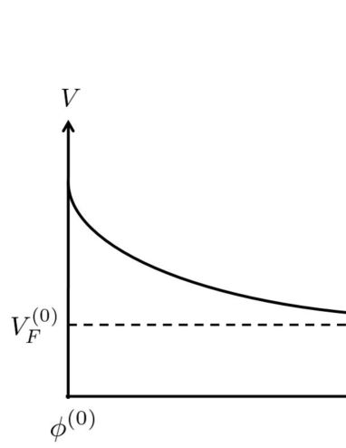
Figure 1: The runaway behavior of the full scalar potential along the direction (3.22).

We give a comment on the roles of the $c_{i}^{(1)}$ and $c_{i}^{(2)}$ terms. It is found from Eqs. (3.23) and (3.24) that, if $c_{i}^{(1)}=c_{i}^{(2)}=0$, the full potential has a constant value $V^{(0)}$ along (3.22). However this neither corresponds to the minimum nor satisfies the stationary condition. The $c^{(1)}$ term drives the potential to a lower value and the $c^{(2)}$ term stabilizes the potential. The detail of the potential analysis in the direction (3.22) is given in Appendix.

For the most generic form of the generalized O’Raifeartaigh models (2.11), the F terms of $X_{i}$ are non-vanishing, $W^{(0)}_{X_{i}}\neq 0$. On top of that, $X_{i}$’s appear as the linear terms in the superpotential and identically satisfy $W_{\phi XX}=0$. Therefore the conditions (3.25) are automatically satisfied if the coefficients $c^{(1)}$ are vanishing for the fields other than $X_{i}$. The other condition (3.26) can be satisfied in the presence of $c^{(1)}_{X_{i}}\neq 0$. Notice that, as mentioned before, some non-vanishing F components of charged fields ($q_{i}W_{i}\neq 0$) are necessarily required by a relation between $F$ and $D$ terms. In the end, the full scalar potential becomes

$$V\to\sum_{i}\big{|}W_{i}^{(0)}\big{|}^{2}\qquad(z_{\infty}\to\infty)\ ,$$ (3.27)

which saturates the lower bound, and the vacuum runs away to infinity.

We conclude that the first class is not relevant for the phenomenological application to gauge mediation. This class leads to unstable potential directions in the SUSY-breaking sector or vanishing gaugino masses at the leading order. The D-term contribution does not work to cure this problem.

3.3.3 Example

We analyze the runaway behavior in a generalized O’Raifeartaigh model with the following superpotential

$$W=X_{0}(f+\lambda\phi_{1}\phi_{2})+m_{1}X_{1}\phi_{1}+m_{2}X_{2}\phi_{2}\ .$$ (3.28)

The model has a U(1) symmetry, which is gauged, and is relevant to our discussion of the D-term effect. We take non-vanishing U(1) charges such that $\phi_{1}$ and $X_{2}$ have $+1$, while $\phi_{2}$ and $X_{1}$ have $-1$. The superpotential is the most generic one for this U(1) symmetry and U(1)_R under which $X_{i}$ ($i=0,1,2$) have charge 2 and the others are zero. All the couplings can be taken real positive by suitable phase rotations up to the U(1) invariance.

Obviously the F-flatness conditions cannot be satisfied simultaneously, and SUSY is broken. We assume $f\lambda>m_{1}m_{2}$ such that the F terms of charged fields $X_{1,2}$ are non-vanishing. As seen below, the D term is also non-vanishing in the vacuum when $m_{1}\neq m_{2}$. The minimum of the F-term scalar potential is found

$$\phi_{1}^{(0)}=-\frac{F}{m_{1}}\ ,\qquad\phi_{2}^{(0)}=\frac{F}{m_{2}}\ ,\qquad X^{(0)}_{0}=X^{(0)}_{1}=X^{(0)}_{2}=0\ ,$$ (3.29)

where we have defined the combinations of couplings as $F\equiv F_{0}\sqrt{(f\lambda/m_{1}m_{2})-1}$ and $F_{0}\equiv m_{1}m_{2}/\lambda$. The expectation values have been made real by the U(1) rotation. At this minimum, the derivatives of the superpotential are

$$W^{(0)}_{\phi_{1}}=W^{(0)}_{\phi_{2}}=0\ ,\qquad W^{(0)}_{X_{0}}=F_{0}\ ,\qquad-W^{(0)}_{X_{1}}=W^{(0)}_{X_{2}}=F\ ,$$ (3.30)

and the resultant minimum of the F-term potential is given by $V^{(0)}_{F}=F_{0}^{2}+2F^{2}$. The F-term potential has the pseudo-moduli direction along $X_{i}=z\overline{W}^{(0)}_{\overline{X}_{i}}$ ($i=0,1,2$).

Let us examine the full scalar potential by adding the D-term contribution. At the minimum of $V_{F}$, the D term is non-vanishing,

$$D=\frac{m_{2}^{2}-m_{1}^{2}}{m_{1}^{2}m_{2}^{2}}\,F^{2}\ ,$$ (3.31)

for $m_{1}\neq m_{2}$. This however does not correspond to the full potential vacuum. Consider a direction parametrized by

$$\phi_{i}=\phi_{i}^{(0)}+\frac{c_{\phi_{i}}^{(2)}}{\bar{z}_{\infty}^{2}}\ ,\qquad X_{0}=z_{\infty}W^{(0)}_{X_{0}}\ ,\qquad X_{i}=z_{\infty}W^{(0)}_{X_{i}}+\frac{c_{X_{i}}^{(1)}}{\bar{z}_{\infty}}+\frac{c_{X_{i}}^{(2)}}{\bar{z}_{\infty}^{2}}\ .$$ (3.32)

It is found that along this direction, the D term approaches to zero in the limit $z_{\infty}\to\infty$ keeping the F terms unchanged, if $c_{X_{i}}^{(1)}$ satisfy

$$\text{Re}\big{(}c_{X_{1}}^{(1)}+c_{X_{2}}^{(1)}\big{)}+\frac{m_{2}^{2}-m_{1}^{2}}{2m_{1}^{2}m_{2}^{2}}\,F=0\ .$$ (3.33)

As a result, the full potential has runaway behavior along the above direction, i.e. $V\to V_{F}^{(0)}$ as $z_{\infty}\to\infty$. The $c^{(2)}$ terms are included to satisfy the stationary conditions as we discuss in Appendix.

3.4 The second class:  Need for the FI term

3.4.1 Scale transformation

The definition of the second class is that all F-flatness conditions, $W_{i}=0$ for $\!{}^{\forall}i$, have some solution, but the D-term contribution destabilizes this minimum of $V_{F}$, which leads to SUSY breaking. In this section, we do not consider the case that the F flatness is satisfied for some infinite values of scalar fields. Such a possibility would be studied elsewhere [13].

We have the U(1) symmetry which acts on $\phi_{i}$ as its phase rotation with the charge $q_{i}$. A key ingredient in this section is that the superpotential is invariant under the following transformation

$$\phi_{i}\to\tau^{q_{i}}\phi_{i}\ ,$$ (3.34)

where $\tau$ is a complex number. That contains a charge-dependent scale transformation as well as the phase rotation. The F terms transform as

$$W_{i}\to\tau^{-q_{i}}W_{i}\ .$$ (3.35)

The solution of F-flatness conditions is denoted by $\phi^{(0)}_{i}$ as before. The transformation (3.35) means that, when $\phi^{(0)}_{i}$ satisfies the F-flatness conditions, $\tau^{q_{i}}\phi^{(0)}_{i}$ is also a solution. We consider two cases separately: (i) the F-flatness conditions are satisfied at the origin of field space, and (ii) the F-flatness requires $\phi^{(0)}_{i}\neq 0$ for some fields. In the second case, the transformation (3.34) acts non-trivially on $\phi_{i}^{(0)}$, which implies that there is a moduli space spanned by $\tau$.

A simple model for the first case has the superpotential

$$W=m\phi_{+}\phi_{-}\ ,$$ (3.36)

where $\phi_{\pm}$ are assumed to have the U(1) charges $\pm 1$. The solution for $W_{\phi_{\pm}}=0$ is $\phi_{\pm}=0$, i.e. the origin of field space. The second case is described, for example, by the superpotential

$$W=X(f+\lambda\phi_{+}\phi_{-})\ ,$$ (3.37)

where $X$ and $\phi_{\pm}$ have the U(1) charges 0 and $\pm 1$, respectively. The solution for the F-flatness conditions is

$$X=0\ ,\qquad\phi_{+}=\tau\phi^{(0)}\ ,\qquad\phi_{-}=\tau^{-1}\phi^{(0)}\ ,$$ (3.38)

where $\phi^{(0)}=\sqrt{-{f}/\lambda}$, and $\tau$ is an arbitrary complex number.

3.4.2 Including the D term

Let us consider the effect of D-term potential by gauging the U(1) symmetry. For the first case, the F-flatness solution $\phi^{(0)}_{i}=0$ leads to $D=0$ without the FI term. It is thus found that a simple SUSY-breaking model for the present purpose is given by (3.36) with a non-vanishing FI term. This model is expected to satisfy the phenomenological requirement that the gaugino mass is generated at one-loop order on the vacuum of full scalar potential. We will discuss the gauge mediation of this type of SUSY breaking in the next section.

For the second case, the F-flatness conditions have the moduli direction $\tau^{q_{i}}\phi^{(0)}_{i}$ with $\tau$ being a free parameter, and there the D term is evaluated as

$$D=\xi+\sum_{i}q_{i}|\tau|^{2q_{i}}\big{|}\phi^{(0)}_{i}\big{|}^{2}\ ,$$ (3.39)

where $\xi$ is the coefficient of the FI term. Suppose that all of fields with non-vanishing $\phi^{(0)}$ have positive (negative) U(1) charges. Then, SUSY is found to be broken for a positive (negative) value of $\xi$. If $\xi=0$, the D-flatness condition requires $\tau=0$ ($\tau\to\infty$), and the full potential has the SUSY-preserving vacuum.

For the remaining case that fields with non-vanishing $\phi^{(0)}$ have positive and negative U(1) charges, SUSY is unbroken. This is because, for a sufficiently small (large) value of $|\tau|$, the D term (3.39) is dominated by negative (positive) charged fields and becomes negative (positive), and therefore $D=0$ has a solution for a finite value of $|\tau|$. For example, the model with the superpotential (3.37) and gauged U(1) symmetry has the D term in the F-flat direction,

$$D=\xi+(|\tau|^{2}-|\tau|^{-2})\big{|}\phi^{(0)}\big{|}^{2}\ .$$ (3.40)

The SUSY vacuum is then given by $|\phi_{\pm}|^{2}=\big{(}\sqrt{\xi^{2}+4|\phi^{(0)}|^{2}}\mp\xi\big{)}/2$.

To summarize, the second class of SUSY-breaking models should have the non-vanishing FI term. We also note that SUSY is unbroken when both positive and negative-charged scalar fields develop non-vanishing expectation values.

4 Gaugino mass generation

In the previous section, we have classified SUSY-breaking models with both F and D-term potentials being relevant, and shown that SUSY breaking is realized in the second class of models with a non-vanishing FI term. Since the argument by Komargodski and Shih is not valid in the D-term extension, these models can be applied to the SUSY-breaking sector of gauge mediation, which generates gaugino masses at one-loop order.

We consider the model with the following superpotential and the D term

$$W_{\cancel{\rm SUSY}}=m\phi_{+}\phi_{-}\ ,\qquad D=\xi+|\phi_{+}|^{2}-|\phi_{-}|^{2}\ .$$ (4.1)

The chiral superfields $\phi_{\pm}$ carry the U(1) charges $\pm 1$. This model belongs to the second class in our classification. Assuming $g^{2}\xi>|m|^{2}$, we obtain the SUSY-breaking vacuum

$$\langle\phi_{+}\rangle=0\ ,\qquad|\langle\phi_{-}\rangle|=\sqrt{\xi-\frac{|m|^{2}}{g^{2}}}\ ,$$ (4.2)

and the F and D components are

$$F_{\phi_{-}}=0\ ,\qquad F_{\phi_{+}}=-m^{*}\langle\bar{\phi}_{-}\rangle\ ,\qquad D=\frac{|m|^{2}}{g^{2}}\ .$$ (4.3)

This is nothing but the Fayet-Iliopoulos model [12] for SUSY breaking.

We next introduce the messenger sector to mediate the SUSY breaking to the visible sector via the standard-model gauge interactions. The messenger chiral multiplets $M$, $\tilde{M}$, $N$, $\tilde{N}$ are charged under the U(1) symmetry and the quantum numbers are shown in Table 2.

	$M$	$\tilde{M}$	$N$	$\tilde{N}$
U(1)	0	0	1	$-1$
$G_{\text{SM}}$	$R$	$R^{*}$	$R$	$R^{*}$

Table 2: The quantum numbers of the messenger multiplets. The symbol $R$ means the representation $R$ of the standard model group $G_{\text{SM}}$.

As mentioned before, the non-vanishing D term requires charged F terms and then implies two pairs of vector-like chiral multiplets as the minimal set of messengers. We have the superpotential for the messenger fields,

$$W_{\text{mess}}=\lambda_{+}\phi_{+}M\tilde{N}+\lambda_{-}\phi_{-}\tilde{M}N+m_{M}M\tilde{M}+m_{N}N\tilde{N}\ .$$ (4.4)

When the messenger mass scales are such that $|m_{M}|,\,|m_{N}|\gg|m|$, the vacuum (4.2) remains stable and the standard-model gauge group is unbroken. As a result, the SUSY-breaking F terms are still given by (4.3) and the bosonic mass-squared matrix for the messengers becomes

$$\begin{pmatrix}M\\ \bar{\tilde{M}}\\ N\\ \bar{\tilde{N}}\end{pmatrix}^{\dagger}\!\!\begin{pmatrix}|m_{M}|^{2}&&m_{M}^{*}\lambda_{-}\langle\phi_{-}\rangle&-\lambda_{+}^{*}F_{\phi_{+}}^{*}\\ &\!|m_{M}|^{2}\!+\!|\lambda_{-}\langle\phi_{-}\rangle|^{2}\!&&\lambda_{-}m_{N}^{*}\langle\phi_{-}\rangle\\ m_{M}\lambda_{-}^{*}\langle\bar{\phi}_{-}\rangle&&\!|m_{N}|^{2}\!+\!|m|^{2}\!+\!|\lambda_{-}\langle\phi_{-}\rangle|^{2}\!\!&\\ -\lambda_{+}F_{\phi_{+}}&\lambda_{-}^{*}m_{N}\langle\bar{\phi}_{-}\rangle&&\!|m_{N}|^{2}\!-\!|m|^{2}\end{pmatrix}\!\begin{pmatrix}M\\ \bar{\tilde{M}}\\ N\\ \bar{\tilde{N}}\end{pmatrix}.$$ (4.5)

For a small SUSY breaking $|F_{\phi_{+}}|\ll|m_{M,N}|^{2}$, the gaugino mass $M_{\tilde{g}}$ in the visible sector is generated through the one-loop diagrams (Figure 2) and evaluated as

$$M_{\tilde{g}}=\frac{g_{\text{SM}}^{2}}{8\pi^{2}}\,T_{2}(R)\lambda_{+}\lambda_{-}\frac{F_{\phi_{+}}\langle\phi_{-}\rangle}{m_{M}m_{N}}\ ,$$ (4.6)

where $g_{\text{SM}}$ is the gauge coupling of the standard model group and $T_{2}(R)$ denotes the Dynkin index for the messenger representation $R$. While the diagrams in Figure 2 are expressed in terms of the mass insertion method, the result of gaugino mass (4.6) is easily shown to be independent of it and exact in the leading order. The result explicitly shows that, in SUSY-breaking models with both F and D terms, one can indeed circumvent the argument in [3] and generate gaugino masses at the one-loop order of gauge mediation.

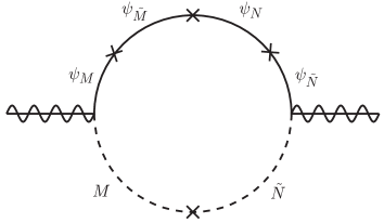
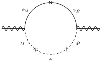
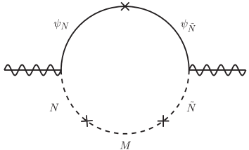
Figure 2: One-loop diagrams for gaugino masses. The symbol $\psi_{x}$ denotes the corresponding superpartner of the scalar $x$.

5 Summary

In this paper we have systematically studied the SUSY-breaking models with F and abelian D terms. The analysis has been performed with the canonical Kähler form and the tree-level scalar potential. The models are classified under the condition whether there exist a F-flatness solution or not. The first class of models has no solution for the F-flatness conditions, i.e. F-term SUSY breaking, and the second one has a solution which is destabilized by the D term in the full potential.

In the first class of models, there exists a pseudo-moduli direction in the F-term scalar potential as studied in [1, 2, 3]. This direction could be lifted in the full scalar potential by a non-vanishing D term with finite values of scalar fields. We have however shown that there is a runaway direction in the full potential and the D term goes to zero. In the second class of models, SUSY breaking requires a FI term added with a proper coefficient. Applying a simple model in the latter class to the gauge mediation, the visible-sector gaugino mass is found to be generated on the stable vacuum at the one-loop order.

Acknowledgment

The authors thank T. Okada for useful discussions. T.A. is supported by Japan Society for the Promotion of Science (JSPS) and Special Postdoctoral Researchers Program at RIKEN. T.K. and K.Y. are supported in part by the Grant-in-Aid for Scientific Research Nos. 20540266 and 23740187, and for the Global COE Program ”The Next Generation of Physics, Spun from Universality and Emergence” from the Ministry of Education, Culture, Sports, Science and Technology of Japan. K.Y. is also supported by Keio Gijuku Academic Development Funds.

Appendix A Stationary conditions

We here examine the stationary conditions of the potential along the direction (3.22). The first derivatives of the F and D-term potentials with respect to $\bar{\phi}_{i}$ are evaluated as

$$(V_{F})_{\bar{i}} =\sum_{j}\Big{(}\sum_{\ell}W_{j\ell}^{(0)}c_{\ell}^{(1)}+\omega^{2}\sum_{\ell,m}W_{j\ell m}^{(0)}\overline{W}_{\bar{\ell}}^{(0)}c_{m}^{(2)}\Big{)}\sum_{k}\overline{W}_{\bar{i}\bar{j}\bar{k}}^{(0)}W_{k}^{(0)}+{\cal O}\Big{(}\frac{1}{z_{\infty}}\Big{)}\ ,$$ (A.1)

$$(V_{D})_{\bar{i}} =g^{2}\omega q_{i}\overline{W}_{\bar{i}}^{(0)}\Big{[}\sum_{j}\omega q_{j}\big{(}\bar{\phi}_{j}^{(0)}c_{j}^{(1)}+W_{j}^{(0)}c_{j}^{(2)}\big{)}+\text{c.c.}\Big{]}+{\cal O}\Big{(}\frac{1}{z_{\infty}}\Big{)}\ ,$$ (A.2)

where we have used the field identities (3.4) and (3.11), and also the minimum conditions of $V_{F}$, i.e. Eqs. (2.4) and (2.8). The coefficients $c^{(1)}_{i}$ satisfy the equations (3.25) and (3.26) so that (3.22) is a runaway direction. As for the generic form (2.11), the superpotential is linear in $X_{i}$ and the F terms of $\phi_{j}$ are assumed to be zero, and we find

$$(V_{F})_{\bar{X}_{i}} =0\ ,$$ (A.3)

$$(V_{F})_{\bar{\phi}_{i}}\, =\sum_{\phi_{j}}\Big{(}\sum_{X_{\ell}}W_{\phi_{j}X_{\ell}}^{(0)}c_{X_{\ell}}^{(1)}+\omega^{2}\!\!\sum_{X_{\ell},\phi_{m}}W_{\phi_{j}\phi_{m}X_{\ell}}^{(0)}\!\overline{W}_{\bar{X}_{\ell}}^{(0)}c_{\phi_{m}}^{(2)}\Big{)}\sum_{X_{k}}\overline{W}_{\bar{\phi}_{i}\bar{\phi}_{j}\bar{X}_{k}}^{(0)}W_{X_{k}}^{(0)}\ ,$$ (A.4)

$$(V_{D})_{\bar{X}_{i}} =g^{2}\omega q_{X_{i}}\overline{W}_{\bar{X}_{i}}^{(0)}\Big{[}\sum_{X_{j}}\omega q_{X_{j}}\big{(}\bar{X}_{j}^{(0)}c_{X_{j}}^{(1)}+W_{X_{j}}^{(0)}c_{X_{j}}^{(2)}\big{)}+\text{c.c.}\Big{]}\ ,$$ (A.5)

$$(V_{D})_{\bar{\phi}_{i}}\, =0\ ,$$ (A.6)

up to ${\cal O}(1/z_{\infty})$. Notice that some combination of $c_{X_{i}}^{(1)}$’s are determined by the runaway conditions of the potential and expressed with $\phi^{(0)}$, and generally $c^{(2)}$ are free parameters. As a result, in the direction (3.22), the stationary conditions for the full potential can be satisfied; $V_{i}=(V_{F})_{i}+(V_{D})_{i}=0+{\cal O}(1/z_{\infty})$ with properly fixed $c^{(2)}$ (and also $c^{(1)}$ consistent with the runaway behavior). The number of parameters is clearly large enough to have a solution for the conditions $V_{i}=0$.

As an example, we discuss the stationary conditions for the model in Section 3.3.3. Along the direction (3.32) with a real $z_{\infty}$, we find the stationary conditions of the full potential

$$V_{\bar{X}_{i}} =2g^{2}F^{2}\,\text{Re}\big{(}c_{X_{1}}^{(2)}+c_{X_{2}}^{(2)}\big{)}=0\ ,\qquad(i=1,2)$$ (A.7)

$$V_{\bar{\phi}_{1}} =m_{1}m_{2}^{2}\big{(}c_{X_{2}}^{(1)}+m_{1}c_{\phi_{1}}^{(2)}\big{)}=0\ ,$$ (A.8)

$$V_{\bar{\phi}_{2}} =m_{1}^{2}m_{2}\big{(}c_{X_{1}}^{(1)}+m_{2}c_{\phi_{2}}^{(2)}\big{)}=0\ ,$$ (A.9)

by explicitly writing down Eqs. (A.4) and (A.5). The condition for the charge-neutral field $X_{0}$ is trivial. Together with the runaway condition (3.33), they give 6 conditions among 12 real parameters, $c^{(1)}_{X_{i}}$, $c^{(2)}_{X_{i}}$, and $c^{(2)}_{\phi_{i}}$. We thus find runaway solutions, an example of which is described by

$$\phi_{1} =-\frac{F}{m_{1}}\ ,$$ (A.10)

$$\phi_{2} =+\frac{F}{m_{2}}+\frac{1}{z_{\infty}^{2}}\,\frac{m_{2}^{2}-m_{1}^{2}}{2m_{1}^{2}m_{2}^{3}}\,F\ ,$$ (A.11)

$$X_{0} =z_{\infty}F_{0}\ ,$$ (A.12)

$$X_{1} =-z_{\infty}F-\frac{1}{z_{\infty}}\,\frac{m_{2}^{2}-m_{1}^{2}}{2m_{1}^{2}m_{2}^{2}}\,F\ ,$$ (A.13)

$$X_{2} =+z_{\infty}F\ .$$ (A.14)

References

- [1] S. Ray, Phys. Lett. B 642, 137 (2006) [arXiv:hep-th/0607172].
- [2] Z. Sun, Nucl. Phys. B 815, 240 (2009) [arXiv:0807.4000 [hep-th]].
- [3] Z. Komargodski and D. Shih, JHEP 0904, 093 (2009) [arXiv:0902.0030 [hep-th]].
- [4] G. F. Giudice and R. Rattazzi, Phys. Rept. 322, 419 (1999) [arXiv:hep-ph/9801271].
- [5] K. I. Izawa, Y. Nomura, K. Tobe and T. Yanagida, Phys. Rev. D 56, 2886 (1997) [arXiv:hep-ph/9705228].
- [6] R. Kitano, H. Ooguri and Y. Ookouchi, Phys. Rev. D 75, 045022 (2007) [arXiv:hep-ph/0612139]; C. Csaki, Y. Shirman and J. Terning, JHEP 0705, 099 (2007) [arXiv:hep-ph/0612241]; S. Abel, C. Durnford, J. Jaeckel and V. V. Khoze, Phys. Lett. B 661, 201 (2008) [arXiv:0707.2958 [hep-ph]]; N. Haba and N. Maru, Phys. Rev. D 76, 115019 (2007) [arXiv:0709.2945 [hep-ph]]; R. Essig, J. F. Fortin, K. Sinha, G. Torroba and M. J. Strassler, JHEP 0903, 043 (2009) [arXiv:0812.3213 [hep-th]].
- [7] Y. Nakai and Y. Ookouchi, JHEP 1101, 093 (2011) [arXiv:1010.5540 [hep-th]].
- [8] G. F. Giudice, M. A. Luty, H. Murayama and R. Rattazzi, JHEP 9812, 027 (1998) [arXiv:hep-ph/9810442]; L. Randall and R. Sundrum, Nucl. Phys. B 557, 79 (1999) [arXiv:hep-th/9810155].
- [9] A. Pomarol and R. Rattazzi, JHEP 9905, 013 (1999) [arXiv:hep-ph/9903448]; R. Rattazzi, A. Strumia and J. D. Wells, Nucl. Phys. B 576, 3 (2000) [arXiv:hep-ph/9912390]; R. Sundrum, Phys. Rev. D 71, 085003 (2005) [arXiv:hep-th/0406012]; K. Hsieh and M. A. Luty, JHEP 0706, 062 (2007) [arXiv:hep-ph/0604256]; M. Endo and K. Yoshioka, Phys. Rev. D 78, 025012 (2008) [arXiv:0804.4192 [hep-ph]]; T. Kobayashi, Y. Nakai and M. Sakai, JHEP 1106, 039 (2011) [arXiv:1103.4912 [hep-ph]].
- [10] K. A. Intriligator, N. Seiberg and D. Shih, JHEP 0707, 017 (2007) [arXiv:hep-th/0703281].
- [11] For example, M. Luo and S. Zheng, JHEP 0901, 004 (2009) [arXiv:0812.4600 [hep-ph]]; L. F. Matos, arXiv:0910.0451 [hep-ph]; K. Intriligator and M. Sudano, JHEP 1006, 047 (2010) [arXiv:1001.5443 [hep-ph]]; T. T. Dumitrescu, Z. Komargodski and M. Sudano, JHEP 1011, 052 (2010) [arXiv:1007.5352 [hep-th]].
- [12] P. Fayet and J. Iliopoulos, Phys. Lett. B 51 (1974) 461.
- [13] Work in progress.