On-shell renormalization of neutralino and chargino mass matrices in R𝑅R-parity violating models - Correlation between LSP decays and neutrino mixing angles revisited

Stefan Liebler sliebler@physik.uni-wuerzburg.de Werner Porod porod@physik.uni-wuerzburg.de Institut für Theoretische Physik und Astrophysik, Universität Würzburg,
D-97074 Würzburg, Germany
Abstract

We present an on-shell renormalization scheme for the neutralino and chargino mass matrices for two R𝑅R-parity violating models, namely bilinear R𝑅R-parity violation and the μν𝜇𝜈\mu\nuSSM with one right-handed neutrino superfield. We discuss in both models how to obtain neutrino masses and mixing angles correctly as well as differences to the existing DR¯¯DR\overline{\text{DR}} calculations. Both models predict correlations between neutrino mixing angles and ratios of R𝑅R-parity violating decays such as χ~10l±Wsuperscriptsubscript~𝜒10superscript𝑙plus-or-minussuperscript𝑊minus-or-plus\tilde{\chi}_{1}^{0}\rightarrow l^{\pm}W^{\mp} which can be tested for example at the LHC. We point out that there are cases where one has to include the complete NLO corrections for the decays χ~10l±Wsuperscriptsubscript~𝜒10superscript𝑙plus-or-minussuperscript𝑊minus-or-plus\tilde{\chi}_{1}^{0}\rightarrow l^{\pm}W^{\mp} to predict reliably the correlations between neutrino- and collider-physics. Moreover, we discuss briefly the implementation of these decays in the public program CNNDecays.

1 Introduction

The Minimal Supersymmetric extension of the Standard Model (MSSM) [1] is based on conserved R𝑅R-parity, where R𝑅R-parity (Rpsubscript𝑅𝑝R_{p}) [2] is defined as Rp=(1)3B+L+2ssubscript𝑅𝑝superscript13𝐵𝐿2𝑠R_{p}=(-1)^{3B+L+2s} and originally guaranteed the stability of the proton in supersymmetric models [3]. It implies on the one hand a stable lightest supersymmetric particle (LSP) and predicts on the other hand zero neutrino masses as in the Standard Model (SM). As neutrino oscillation experiments have shown at least two neutrinos have non-zero mass [4] requiring an extension to explain neutrino data111A recent analysis combining the newest precision results from various experiments like KamLAND [5], Super-K [6], SAGE [7], SNO [8] or MINOS [9] can be found in Ref. [10]..

In the SM exist various ways to explain neutrino data, e.g. postulating very heavy particles as in the seesaw mechanism [11, 12] resulting in a unique dimension-5 operator [13] or via loop-effects [12, 14, 15]. Although all mentioned solutions can be supersymmetrized, there exists an entirely supersymmetric possibility to generate Majorana neutrino masses, namely R𝑅R-parity violation Rp/R_{p}/\;\>\hskip 1.99997pt[16, 17, 18]. Allowing for all possible gauge- and supersymmetric invariant terms within the MSSM particle content, R𝑅R-parity can be broken by bilinear or trilinear terms [17]. Trilinear models provide a huge number of free parameters, where different attempts tried to reduce them [19]. Spontaneous R𝑅R-parity violation can be understood as a violation of lepton number by the vacuum expectation value of some singlet field [16, 20, 21]. Bilinear Rp/R_{p}/\;\>\hskip 1.99997ptcan be interpreted as the low-energy limit of some spontaneous Rp/R_{p}/\;\>\hskip 1.99997ptmodel, where the new singlet fields are all decoupled. The bilinear model has only six new Rp/R_{p}/\;\>\hskip 1.99997ptparameters and is thus more predictive in particular in view of collider physics once the parameters have been chosen to explain correctly neutrino data. For an early work on bilinear R𝑅R-parity violation in the context of a low-energy effective theory we refer to [22].

The phenomenology of Rp/R_{p}/\;\>\hskip 1.99997ptSUSY has been studied extensively in the past, for reviews see [23, 24, 25]. Neutrino masses have been calculated with trilinear couplings [17, 26] and for pure bilinear models [27, 28, 29, 30, 31] or both [32]. Neutrino angles are not predicted in either schemes, but can be easily fitted to experimental data. In bilinear schemes the requirement to correctly explain neutrino data fixes all Rp/R_{p}/\;\>\hskip 1.99997ptcouplings in sufficiently small intervals, so that in some specific final states of the decays of the LSP correlations with neutrino angles appear. This has been shown for a (bino-dominated) neutralino LSP in [33, 34, 35], for charged scalar LSPs in [36], for sneutrino LSPs in [37, 38], and for chargino, gluino and squark LSPs in [37]. Such a tight connection between neutrino physics and LSP decays is lost to some extent in the general trilinear-plus-bilinear case.

The μ𝜇\mu-problem of the MSSM [39] is induced by the mass term for the Higgs superfields μH^dH^u𝜇subscript^𝐻𝑑subscript^𝐻𝑢\mu\widehat{H}_{d}\widehat{H}_{u}. For phenomenological reasons the parameter μ𝜇\mu must be of the order of the electroweak scale. However, if there is a larger scale in the theory, the natural value of μ𝜇\mu should be around this large scale. A solution to this problem can be provided by the Next-to-Minimal SSM (NMSSM) [40, 41], where an additional singlet superfield is introduced. The vacuum expectation value of its scalar component generates an effective μ𝜇\mu term as soon as electroweak symmetry is broken. The phenomenology has been discussed for example in [42, 43]. Electroweak mass corrections were discussed in [44], an on-shell scheme for neutralino and chargino masses including the discussion of the two-body decays χ~i0χ~j±Wsuperscriptsubscript~𝜒𝑖0superscriptsubscript~𝜒𝑗plus-or-minussuperscript𝑊minus-or-plus\tilde{\chi}_{i}^{0}\rightarrow\tilde{\chi}_{j}^{\pm}W^{\mp} at one-loop level was worked out in [45].

The μν𝜇𝜈\mu\nuSSM, which was first proposed in [46], uses the same singlet superfield(s) not only to generate the μ𝜇\mu term but in addition Dirac mass terms for the left-handed neutrinos. The cubic self-couplings of the singlets in the superpotential explicitly break lepton number and moreover also Rpsubscript𝑅𝑝R_{p}. Thus, Majorana neutrino masses are generated once electroweak symmetry is broken. One-loop corrections to the neutrino mass matrix have been calculated in [47, 48]. Compared to the NMSSM the μν𝜇𝜈\mu\nuSSM with one right-handed neutrino superfield also contains six new Rp/R_{p}/\;\>\hskip 1.99997ptparameters, the same number as going from the MSSM to the bilinear Rp/R_{p}/\;\>\hskip 1.99997ptmodel as will be discussed in detail later on. This implies that one also obtains correlations between neutrino mixing angles and ratios of LSP decay branching ratios [47, 49]. Moreover, one has unusual decay modes and signatures in the Higgs sector [47, 50].

Although one expects correlations between neutrino mixing angles and final states of the LSP decays at tree level, it is a priori unclear what happens at one-loop level. In particular using one-loop on-shell masses and the one-loop mixing matrix together with the tree level decay widths results in case of the μν𝜇𝜈\mu\nuSSM with one right-handed neutrino superfield in an unexpected behavior: The expected correlation does not necessarily show up for a singlino-like LSP. Therefore, we present in this paper a full one-loop calculation for the decays χ~10l±Wsuperscriptsubscript~𝜒10superscript𝑙plus-or-minussuperscript𝑊minus-or-plus\tilde{\chi}_{1}^{0}\rightarrow l^{\pm}W^{\mp} and show how the tree level expectations evolve at full one-loop level. For this aim we extend the on-shell scheme presented in [45] for the decays χ~i0χ~j±Wsuperscriptsubscript~𝜒𝑖0superscriptsubscript~𝜒𝑗plus-or-minussuperscript𝑊minus-or-plus\tilde{\chi}_{i}^{0}\rightarrow\tilde{\chi}_{j}^{\pm}W^{\mp} within the MSSM and the NMSSM to the models considered here. Moreover, we briefly discuss the implementation of these decays in CNNDecays [51]. Note that in case of the μν𝜇𝜈\mu\nuSSM with more than one right-handed neutrino superfield similar problems do not show up. The reason is, that neutrino physics can be fully explained at tree level and thus at the same level of perturbation theory as the correlations with the neutralino branching ratios.

This paper is organized as follows: We first define our models in Section 2. In Section 3 we present our on-shell scheme for the neutralino and chargino mass matrices in the considered models. Afterwards we present numerical results for the neutrino masses and mixings comparing the on-shell scheme and the DR¯¯DR\overline{\text{DR}} scheme in Section 4. Next we discuss the decays χ~10l±Wsuperscriptsubscript~𝜒10superscript𝑙plus-or-minussuperscript𝑊minus-or-plus\tilde{\chi}_{1}^{0}\rightarrow l^{\pm}W^{\mp} and the correlations to neutrino physics at tree level in Section 5. In Section 6 we first discuss the complete NLO corrections to the widths and discuss the correlations at one-loop level. Finally we conclude in Section 7. A gives the implementation of the considered models in the public program CNNDecays.

2 Model definition

In this section we introduce the models by presenting the superpotential and the soft-breaking terms. Moreover we will give the neutralino and chargino mass matrices at tree level and comment on the need of one-loop corrections for the neutrino masses.

2.1 Superpotential, soft terms and scalar potential

We will start with the superpotential of bilinear R𝑅R-parity violation (BRpV) and the μν𝜇𝜈\mu\nuSSM with one right-handed neutrino superfield ν^csuperscript^𝜈𝑐\widehat{\nu}^{c}. Both model have in common the Yukawa part of the matter superfields coupled to the SU(2)𝑆𝑈2SU(2)-doublet Higgs fields

𝒲Y=ϵαβ(YUijQ^iαu^jcH^uβ+YDijQ^iβd^jcH^dα+YlijL^iβl^jcH^dα),subscript𝒲𝑌subscriptitalic-ϵ𝛼𝛽superscriptsubscript𝑌𝑈𝑖𝑗superscriptsubscript^𝑄𝑖𝛼superscriptsubscript^𝑢𝑗𝑐superscriptsubscript^𝐻𝑢𝛽superscriptsubscript𝑌𝐷𝑖𝑗superscriptsubscript^𝑄𝑖𝛽superscriptsubscript^𝑑𝑗𝑐superscriptsubscript^𝐻𝑑𝛼superscriptsubscript𝑌𝑙𝑖𝑗superscriptsubscript^𝐿𝑖𝛽superscriptsubscript^𝑙𝑗𝑐superscriptsubscript^𝐻𝑑𝛼\displaystyle{\cal W}_{Y}=\epsilon_{\alpha\beta}\left(Y_{U}^{ij}\widehat{Q}_{i}^{\alpha}\widehat{u}_{j}^{c}\widehat{H}_{u}^{\beta}+Y_{D}^{ij}\widehat{Q}_{i}^{\beta}\widehat{d}_{j}^{c}\widehat{H}_{d}^{\alpha}+Y_{l}^{ij}\widehat{L}_{i}^{\beta}\widehat{l}_{j}^{c}\widehat{H}_{d}^{\alpha}\right)\qquad, (1)

where ϵαβsubscriptitalic-ϵ𝛼𝛽\epsilon_{\alpha\beta} is the complete antisymmetric SU(2)𝑆𝑈2SU(2) tensor with ϵ12=1subscriptitalic-ϵ121\epsilon_{12}=1 and i,j𝑖𝑗i,j denote the three families. In case of BRpV the explicit μ𝜇\mu and ϵisubscriptitalic-ϵ𝑖\epsilon_{i}-terms are added and the total superpotential reads as

𝒲bRp/=𝒲Y+ϵαβ[ϵiL^iαH^uβμH^dαH^uβ],\displaystyle{\cal W}_{b\text{$R_{p}/\;\>\hskip 1.39998pt$}}={\cal W}_{Y}+\epsilon_{\alpha\beta}\left[\epsilon_{i}\widehat{L}_{i}^{\alpha}\widehat{H}_{u}^{\beta}-\mu\widehat{H}_{d}^{\alpha}\widehat{H}_{u}^{\beta}\right]\qquad, (2)

whereas in the μν𝜇𝜈\mu\nuSSM the Higgs doublets are coupled to the right-handed neutrino superfield ν^csuperscript^𝜈𝑐\widehat{\nu}^{c} and in addition a term containing the neutrino Yukawa coupling Yνsubscript𝑌𝜈Y_{\nu} is added

𝒲μνSSM=subscript𝒲𝜇𝜈SSMabsent\displaystyle{\cal W}_{\mu\nu\text{SSM}}= 𝒲Y+ϵαβ[YνiL^iαν^cH^uβλν^cH^dαH^uβ]+13κν^cν^cν^c.subscript𝒲𝑌subscriptitalic-ϵ𝛼𝛽delimited-[]superscriptsubscript𝑌𝜈𝑖superscriptsubscript^𝐿𝑖𝛼superscript^𝜈𝑐superscriptsubscript^𝐻𝑢𝛽𝜆superscript^𝜈𝑐superscriptsubscript^𝐻𝑑𝛼superscriptsubscript^𝐻𝑢𝛽13𝜅superscript^𝜈𝑐superscript^𝜈𝑐superscript^𝜈𝑐\displaystyle{\cal W}_{Y}+\epsilon_{\alpha\beta}\left[Y_{\nu}^{i}\widehat{L}_{i}^{\alpha}\widehat{\nu}^{c}\widehat{H}_{u}^{\beta}-\lambda\widehat{\nu}^{c}\widehat{H}_{d}^{\alpha}\widehat{H}_{u}^{\beta}\right]+\frac{1}{3}\kappa\widehat{\nu}^{c}\widehat{\nu}^{c}\widehat{\nu}^{c}\qquad. (3)

The first term in Equation (2) and the last two terms in Equation (3) explicitly break lepton number if one assigns lepton number to ν^csuperscript^𝜈𝑐\widehat{\nu}^{c}. If not the first term in Equation (3) explicitly breaks lepton number and one immediately sees that in both models one has the same number of Rp/R_{p}/\;\>\hskip 1.99997ptviolating parameters. Note that for the phenomenology it does not matter if ν^csuperscript^𝜈𝑐\widehat{\nu}^{c} carries lepton number as it is broken explicitly by a least one interaction of this field. Both models have in common the soft SUSY breaking terms

VsoftMSSMBμ=superscriptsubscript𝑉𝑠𝑜𝑓𝑡MSSM𝐵𝜇absent\displaystyle V_{soft}^{\text{MSSM}-B\mu}= mQij2Q~iαQ~jα+mUij2u~icu~jc+mDij2d~icd~jc+mLij2L~iαL~jα+mEij2l~icl~jcsuperscriptsuperscriptsubscript𝑚𝑄𝑖𝑗2superscriptsubscript~𝑄𝑖𝛼superscriptsubscript~𝑄𝑗𝛼superscriptsuperscriptsubscript𝑚𝑈𝑖𝑗2superscriptsubscript~𝑢𝑖𝑐superscriptsubscript~𝑢𝑗𝑐superscriptsuperscriptsubscript𝑚𝐷𝑖𝑗2superscriptsubscript~𝑑𝑖𝑐superscriptsubscript~𝑑𝑗𝑐superscriptsuperscriptsubscript𝑚𝐿𝑖𝑗2superscriptsubscript~𝐿𝑖𝛼superscriptsubscript~𝐿𝑗𝛼superscriptsuperscriptsubscript𝑚𝐸𝑖𝑗2superscriptsubscript~𝑙𝑖𝑐superscriptsubscript~𝑙𝑗𝑐\displaystyle{m_{Q}^{ij}}^{2}\tilde{Q}_{i}^{\alpha\ast}\tilde{Q}_{j}^{\alpha}+{m_{U}^{ij}}^{2}\tilde{u}_{i}^{c}\tilde{u}_{j}^{c\ast}+{m_{D}^{ij}}^{2}\tilde{d}_{i}^{c}\tilde{d}_{j}^{c\ast}+{m_{L}^{ij}}^{2}\tilde{L}_{i}^{\alpha\ast}\tilde{L}_{j}^{\alpha}+{m_{E}^{ij}}^{2}\tilde{l}_{i}^{c}\tilde{l}_{j}^{c\ast}
+mHd2HdaHda+mHu2HuaHua12[M1B~0B~0+M2W~γW~γ+M3g~γg~γ+h.c.]\displaystyle+m_{H_{d}}^{2}H_{d}^{a\ast}H_{d}^{a}+m_{H_{u}}^{2}H_{u}^{a\ast}H_{u}^{a}-\frac{1}{2}\big{[}M_{1}\tilde{B}^{0}\tilde{B}^{0}+M_{2}\tilde{W}^{\gamma}\tilde{W}^{\gamma}+M_{3}\tilde{g}^{\gamma^{\prime}}\tilde{g}^{\gamma^{\prime}}+h.c.\big{]}
+ϵαβ[TUijQ~iαu~jcHuβ+TDijQ~iβd~jcHdα+TEijL~iβl~jcHdα+h.c.],\displaystyle+\epsilon_{\alpha\beta}\big{[}T_{U}^{ij}\tilde{Q}_{i}^{\alpha}\tilde{u}_{j}^{c\ast}H_{u}^{\beta}+T_{D}^{ij}\tilde{Q}_{i}^{\beta}\tilde{d}_{j}^{c\ast}H_{d}^{\alpha}+T_{E}^{ij}\tilde{L}_{i}^{\beta}\tilde{l}_{j}^{c\ast}H_{d}^{\alpha}+h.c.\big{]}\quad, (4)

where VsoftMSSMBμsuperscriptsubscript𝑉𝑠𝑜𝑓𝑡MSSM𝐵𝜇V_{soft}^{\text{MSSM}-B\mu} contains all the usual soft terms of the MSSM but the Bμsubscript𝐵𝜇B_{\mu}-term and a summation over γ=1,,3𝛾13\gamma=1,\ldots,3 and γ=1,,8superscript𝛾18\gamma^{\prime}=1,\ldots,8 has to be performed. In addition we add in case of BRpV

VsoftbRp/=VsoftMSSMBμ+ϵαβ[BiϵiL~iαHuβBμHdαHuβ+h.c.]\displaystyle V_{soft}^{b\text{$R_{p}/\;\>\hskip 1.39998pt$}}=V_{soft}^{\text{MSSM}-B\mu}+\epsilon_{\alpha\beta}\left[B_{i}\epsilon_{i}\tilde{L}_{i}^{\alpha}H_{u}^{\beta}-B\mu H_{d}^{\alpha}H_{u}^{\beta}+h.c.\right] (5)

and in case of the μν𝜇𝜈\mu\nuSSM:

VsoftμνSSM=superscriptsubscript𝑉𝑠𝑜𝑓𝑡𝜇𝜈SSMabsent\displaystyle V_{soft}^{\mu\nu\text{SSM}}= VsoftMSSMBμ+mν~c2ν~cν~csuperscriptsubscript𝑉𝑠𝑜𝑓𝑡MSSM𝐵𝜇superscriptsubscript𝑚superscript~𝜈𝑐2superscript~𝜈𝑐superscript~𝜈𝑐\displaystyle V_{soft}^{\text{MSSM}-B\mu}+{m_{\tilde{\nu}^{c}}}^{2}\tilde{\nu}^{c}\tilde{\nu}^{c\ast}
+ϵαβ[TνiL~iαν~cHuβTλν~cHdαHuβ+h.c.]+[13Tκν~cν~cν~c+h.c.]\displaystyle+\epsilon_{\alpha\beta}\big{[}T_{\nu}^{i}\tilde{L}_{i}^{\alpha}\tilde{\nu}^{c}H_{u}^{\beta}-T_{\lambda}\tilde{\nu}^{c}H_{d}^{\alpha}H_{u}^{\beta}+h.c.\big{]}+\big{[}\frac{1}{3}T_{\kappa}\tilde{\nu}^{c}\tilde{\nu}^{c}\tilde{\nu}^{c}+h.c.\big{]} (6)

In these expressions the notation for the soft trilinear couplings introduced in [52] is used. We will not present the scalar potential and the corresponding tadpole equations in this paper, but refer to [30] for BRpV and to [47] for the μν𝜇𝜈\mu\nuSSM. Note the different definition of κ𝜅\kappa in comparison to [47]. The determination of the vacuum structure through the scalar potential induces the following vacuum expectation values (VEVs):

Hd0=12vd,Hu0=12vu,ν~i=12vi,ν~c=12vcformulae-sequencedelimited-⟨⟩superscriptsubscript𝐻𝑑012subscript𝑣𝑑formulae-sequencedelimited-⟨⟩superscriptsubscript𝐻𝑢012subscript𝑣𝑢formulae-sequencedelimited-⟨⟩subscript~𝜈𝑖12subscript𝑣𝑖delimited-⟨⟩superscript~𝜈𝑐12subscript𝑣𝑐\displaystyle\left<H_{d}^{0}\right>=\frac{1}{\sqrt{2}}v_{d},\qquad\left<H_{u}^{0}\right>=\frac{1}{\sqrt{2}}v_{u},\qquad\left<\tilde{\nu}_{i}\right>=\frac{1}{\sqrt{2}}v_{i},\qquad\left<\tilde{\nu}^{c}\right>=\frac{1}{\sqrt{2}}v_{c} (7)

Again ν~csuperscript~𝜈𝑐\tilde{\nu}^{c} is only present in the μν𝜇𝜈\mu\nuSSM, where its vacuum expectation value generates effective μ𝜇\mu- and ϵisubscriptitalic-ϵ𝑖\epsilon_{i}-terms

μ=12λvc,ϵi=12Yνivc.formulae-sequence𝜇12𝜆subscript𝑣𝑐subscriptitalic-ϵ𝑖12superscriptsubscript𝑌𝜈𝑖subscript𝑣𝑐\displaystyle\mu=\frac{1}{\sqrt{2}}\lambda v_{c},\qquad\epsilon_{i}=\frac{1}{\sqrt{2}}Y_{\nu}^{i}v_{c}\qquad. (8)

In this way ν^csuperscript^𝜈𝑐\widehat{\nu}^{c} plays the role of the singlet superfield S^^𝑆\widehat{S} in the NMSSM, implying that μ𝜇\mu, but also ϵisubscriptitalic-ϵ𝑖\epsilon_{i} is naturally of the order of the electroweak scale [43]. Moreover there are no additional terms with dimension of mass present in the superpotential. Beside the parameter ϵisubscriptitalic-ϵ𝑖\epsilon_{i} we define the so-called alignment parameters

Λi=μvi+vdϵi,subscriptΛ𝑖𝜇subscript𝑣𝑖subscript𝑣𝑑subscriptitalic-ϵ𝑖\displaystyle\Lambda_{i}=\mu v_{i}+v_{d}\epsilon_{i}\qquad, (9)

which determine the neutrino mass matrix at tree level [47] and which give the relevant information on the tree level mass matrix in a basis invariant way [53]. ϵisubscriptitalic-ϵ𝑖\epsilon_{i} and ΛisubscriptΛ𝑖\Lambda_{i} can then be used to fit the neutrino data. Concerning the scalar potential we add, that in case of BRpV we determine the soft-breaking parameters mHd2,mHu2superscriptsubscript𝑚subscript𝐻𝑑2superscriptsubscript𝑚subscript𝐻𝑢2m_{H_{d}}^{2},m_{H_{u}}^{2} and Bisubscript𝐵𝑖B_{i} and in case of the μν𝜇𝜈\mu\nuSSM mHd2,mHu2,mνc2superscriptsubscript𝑚subscript𝐻𝑑2superscriptsubscript𝑚subscript𝐻𝑢2superscriptsubscript𝑚superscript𝜈𝑐2m_{H_{d}}^{2},m_{H_{u}}^{2},m_{\nu^{c}}^{2} and Tνisuperscriptsubscript𝑇𝜈𝑖T_{\nu}^{i} from the tadpole equations.

2.2 Masses of neutralinos and charginos

Using Weyl spinors defined by

(ψ)T=(W~,H~d,e,μ,τ),(ψ+)T=(W~+,H~u+,ec,μc,τc)formulae-sequencesuperscriptsuperscript𝜓𝑇superscript~𝑊superscriptsubscript~𝐻𝑑𝑒𝜇𝜏superscriptsuperscript𝜓𝑇superscript~𝑊superscriptsubscript~𝐻𝑢superscript𝑒𝑐superscript𝜇𝑐superscript𝜏𝑐\displaystyle\left(\psi^{-}\right)^{T}=\left(\tilde{W}^{-},\tilde{H}_{d}^{-},e,\mu,\tau\right),\qquad\left(\psi^{+}\right)^{T}=\left(\tilde{W}^{+},\tilde{H}_{u}^{+},e^{c},\mu^{c},\tau^{c}\right) (10)

the Lagrangian density containing the chargino masses can be written in the form

12((ψ)Tcψ++(ψ+)T(c)Tψ)+h.c.,formulae-sequence12superscriptsuperscript𝜓𝑇subscript𝑐superscript𝜓superscriptsuperscript𝜓𝑇superscriptsubscript𝑐𝑇superscript𝜓𝑐\displaystyle\mathcal{L}\supset-\frac{1}{2}\left((\psi^{-})^{T}\mathcal{M}_{c}\psi^{+}+(\psi^{+})^{T}(\mathcal{M}_{c})^{T}\psi^{-}\right)+h.c.\qquad, (11)

where the mass matrix of the charged fermions is given by

c=(M212gvu00012gvdμ12Yli1vi12Yli2vi12Yli3vi12gv1ϵ112Yl11vd12Yl12vd12Yl13vd12gv2ϵ212Yl21vd12Yl22vd12Yl23vd12gv3ϵ312Yl31vd12Yl32vd12Yl33vd).subscript𝑐matrixsubscript𝑀212𝑔subscript𝑣𝑢00012𝑔subscript𝑣𝑑𝜇12superscriptsubscript𝑌𝑙𝑖1subscript𝑣𝑖12superscriptsubscript𝑌𝑙𝑖2subscript𝑣𝑖12superscriptsubscript𝑌𝑙𝑖3subscript𝑣𝑖12𝑔subscript𝑣1subscriptitalic-ϵ112superscriptsubscript𝑌𝑙11subscript𝑣𝑑12superscriptsubscript𝑌𝑙12subscript𝑣𝑑12superscriptsubscript𝑌𝑙13subscript𝑣𝑑12𝑔subscript𝑣2subscriptitalic-ϵ212superscriptsubscript𝑌𝑙21subscript𝑣𝑑12superscriptsubscript𝑌𝑙22subscript𝑣𝑑12superscriptsubscript𝑌𝑙23subscript𝑣𝑑12𝑔subscript𝑣3subscriptitalic-ϵ312superscriptsubscript𝑌𝑙31subscript𝑣𝑑12superscriptsubscript𝑌𝑙32subscript𝑣𝑑12superscriptsubscript𝑌𝑙33subscript𝑣𝑑\mathcal{M}_{c}=\begin{pmatrix}M_{2}&\frac{1}{\sqrt{2}}gv_{u}&0&0&0\\ \frac{1}{\sqrt{2}}gv_{d}&\mu&-\frac{1}{\sqrt{2}}Y_{l}^{i1}v_{i}&-\frac{1}{\sqrt{2}}Y_{l}^{i2}v_{i}&-\frac{1}{\sqrt{2}}Y_{l}^{i3}v_{i}\\ \frac{1}{\sqrt{2}}gv_{1}&-\epsilon_{1}&\frac{1}{\sqrt{2}}Y_{l}^{11}v_{d}&\frac{1}{\sqrt{2}}Y_{l}^{12}v_{d}&\frac{1}{\sqrt{2}}Y_{l}^{13}v_{d}\\ \frac{1}{\sqrt{2}}gv_{2}&-\epsilon_{2}&\frac{1}{\sqrt{2}}Y_{l}^{21}v_{d}&\frac{1}{\sqrt{2}}Y_{l}^{22}v_{d}&\frac{1}{\sqrt{2}}Y_{l}^{23}v_{d}\\ \frac{1}{\sqrt{2}}gv_{3}&-\epsilon_{3}&\frac{1}{\sqrt{2}}Y_{l}^{31}v_{d}&\frac{1}{\sqrt{2}}Y_{l}^{32}v_{d}&\frac{1}{\sqrt{2}}Y_{l}^{33}v_{d}\end{pmatrix}\quad. (12)

The mass eigenstates are obtained by two unitary matrices U𝑈U and V𝑉V

Fi+=Vitψt+andFi=Uitψt,formulae-sequencesuperscriptsubscript𝐹𝑖subscript𝑉𝑖𝑡superscriptsubscript𝜓𝑡andsuperscriptsubscript𝐹𝑖subscript𝑈𝑖𝑡superscriptsubscript𝜓𝑡\displaystyle F_{i}^{+}=V_{it}\psi_{t}^{+}\quad\text{and}\quad F_{i}^{-}=U_{it}\psi_{t}^{-}\quad, (13)

so that the mass eigenvalues can be calculated via

c,dia.=Diag(mχ~1+,,mχ~5+)subscript𝑐𝑑𝑖𝑎Diagsubscript𝑚superscriptsubscript~𝜒1subscript𝑚superscriptsubscript~𝜒5\displaystyle\mathcal{M}_{c,dia.}=\text{Diag}\left(m_{\tilde{\chi}_{1}^{+}},\ldots,m_{\tilde{\chi}_{5}^{+}}\right) =\displaystyle= UcV1superscript𝑈subscript𝑐superscript𝑉1\displaystyle U^{*}\mathcal{M}_{c}V^{-1} (14)
mχ~i+mχ~j+fori<jformulae-sequencesubscript𝑚superscriptsubscript~𝜒𝑖subscript𝑚superscriptsubscript~𝜒𝑗for𝑖𝑗\displaystyle m_{\tilde{\chi}_{i}^{+}}\leq m_{\tilde{\chi}_{j}^{+}}\qquad\text{for}\qquad i<j

and the Dirac spinor χ~i+superscriptsubscript~𝜒𝑖\tilde{\chi}_{i}^{+} can be deduced from

χ~i+=(Fi+Fi¯).superscriptsubscript~𝜒𝑖superscriptsubscript𝐹𝑖¯subscriptsuperscript𝐹𝑖\tilde{\chi}_{i}^{+}=\left(\begin{array}[]{c}F_{i}^{+}\\ \overline{F^{-}_{i}}\end{array}\right)\qquad. (15)

For the neutralinos we obtain in the basis 222ν^csuperscript^𝜈𝑐\widehat{\nu}^{c} is only present in the μν𝜇𝜈\mu\nuSSM.

(ψ0)Tsuperscriptsuperscript𝜓0𝑇\displaystyle\left(\psi^{0}\right)^{T} =(B~0,W~30,H~d0,H~u0,νc,ν1,ν2,ν3)absentsuperscript~𝐵0superscriptsubscript~𝑊30superscriptsubscript~𝐻𝑑0superscriptsubscript~𝐻𝑢0superscript𝜈𝑐subscript𝜈1subscript𝜈2subscript𝜈3\displaystyle=\left({\tilde{B}}^{0},{\tilde{W}}_{3}^{0},{\tilde{H}}_{d}^{0},{\tilde{H}}_{u}^{0},\nu^{c},\nu_{1},\nu_{2},\nu_{3}\right) (16)

the mass matrices of the neutral fermions, which have the generic structure

n=(MHm^m^T0)subscript𝑛matrixsubscript𝑀𝐻^𝑚superscript^𝑚𝑇0\displaystyle\mathcal{M}_{n}=\begin{pmatrix}M_{H}&\hat{m}\\ \hat{m}^{T}&0\end{pmatrix} (17)

and enter the Lagrangian density 12((ψ0)Tnψ0)+h.c.formulae-sequence12superscriptsuperscript𝜓0𝑇subscript𝑛superscript𝜓0𝑐\mathcal{L}\supset-\frac{1}{2}\left((\psi^{0})^{T}\mathcal{M}_{n}\psi^{0}\right)+h.c.. The submatrix MHsubscript𝑀𝐻M_{H} contains the 4(5)454(5) heavy states, which are the four usual neutralinos of the MSSM and in case of the μν𝜇𝜈\mu\nuSSM in addition the right-handed neutrino. The submatrix m^^𝑚\hat{m} mixes the heavy states with the left-handed neutrinos and contains the R𝑅R-parity breaking parameters. In detail the elements are given by

MH=(M1012gvd12gvu00M212gvd12gvu012gvd12gvd0μ12λvu12gvu12gvuμ012λvd0012λvu12λvd2κvc)subscript𝑀𝐻matrixsubscript𝑀1012superscript𝑔subscript𝑣𝑑12superscript𝑔subscript𝑣𝑢00subscript𝑀212𝑔subscript𝑣𝑑12𝑔subscript𝑣𝑢012superscript𝑔subscript𝑣𝑑12𝑔subscript𝑣𝑑0𝜇12𝜆subscript𝑣𝑢12superscript𝑔subscript𝑣𝑢12𝑔subscript𝑣𝑢𝜇012𝜆subscript𝑣𝑑0012𝜆subscript𝑣𝑢12𝜆subscript𝑣𝑑2𝜅subscript𝑣𝑐\displaystyle M_{H}=\begin{pmatrix}M_{1}&0&-\frac{1}{2}g^{\prime}v_{d}&\frac{1}{2}g^{\prime}v_{u}&0\\ 0&M_{2}&\frac{1}{2}gv_{d}&-\frac{1}{2}gv_{u}&0\\ -\frac{1}{2}g^{\prime}v_{d}&\frac{1}{2}gv_{d}&0&-\mu&-\frac{1}{\sqrt{2}}\lambda v_{u}\\ \frac{1}{2}g^{\prime}v_{u}&-\frac{1}{2}gv_{u}&-\mu&0&-\frac{1}{\sqrt{2}}\lambda v_{d}\\ 0&0&-\frac{1}{\sqrt{2}}\lambda v_{u}&-\frac{1}{\sqrt{2}}\lambda v_{d}&\sqrt{2}\kappa v_{c}\end{pmatrix} (18)
m^T=(12gv112gv10ϵ1ϵ1vuvc12gv212gv20ϵ2ϵ2vuvc12gv312gv30ϵ3ϵ3vuvc),superscript^𝑚𝑇matrix12superscript𝑔subscript𝑣112𝑔subscript𝑣10subscriptitalic-ϵ1subscriptitalic-ϵ1subscript𝑣𝑢subscript𝑣𝑐12superscript𝑔subscript𝑣212𝑔subscript𝑣20subscriptitalic-ϵ2subscriptitalic-ϵ2subscript𝑣𝑢subscript𝑣𝑐12superscript𝑔subscript𝑣312𝑔subscript𝑣30subscriptitalic-ϵ3subscriptitalic-ϵ3subscript𝑣𝑢subscript𝑣𝑐\displaystyle\hat{m}^{T}=\begin{pmatrix}-\frac{1}{2}g^{\prime}v_{1}&\frac{1}{2}gv_{1}&0&\epsilon_{1}&\epsilon_{1}\frac{v_{u}}{v_{c}}\\ -\frac{1}{2}g^{\prime}v_{2}&\frac{1}{2}gv_{2}&0&\epsilon_{2}&\epsilon_{2}\frac{v_{u}}{v_{c}}\\ -\frac{1}{2}g^{\prime}v_{3}&\frac{1}{2}gv_{3}&0&\epsilon_{3}&\epsilon_{3}\frac{v_{u}}{v_{c}}\end{pmatrix}\qquad, (19)

where in the μν𝜇𝜈\mu\nuSSM μ𝜇\mu and ϵisubscriptitalic-ϵ𝑖\epsilon_{i} can be taken from Equation (8). In case of BRpV one has to omit the last column and the last row in the submatrix MHsubscript𝑀𝐻M_{H} and the last column in the matrix m^^𝑚\hat{m}. The mass eigenstates Fi0superscriptsubscript𝐹𝑖0F_{i}^{0} are obtained via

Fi0=𝒩isψs0superscriptsubscript𝐹𝑖0subscript𝒩𝑖𝑠superscriptsubscript𝜓𝑠0F_{i}^{0}=\mathcal{N}_{is}\psi_{s}^{0} (20)

from the gauge eigenstates ψs0superscriptsubscript𝜓𝑠0\psi_{s}^{0}, where the unitary matrix 𝒩𝒩\mathcal{N} diagonalizes the mass matrix nsubscript𝑛\mathcal{M}_{n} as

n,dia.=Diag(mχ~10,,mχ~j0)=𝒩n𝒩,subscript𝑛𝑑𝑖𝑎Diagsubscript𝑚superscriptsubscript~𝜒10subscript𝑚superscriptsubscript~𝜒𝑗0superscript𝒩subscript𝑛superscript𝒩\mathcal{M}_{n,dia.}=\text{Diag}\left(m_{\tilde{\chi}_{1}^{0}},\ldots,m_{\tilde{\chi}_{j}^{0}}\right)=\mathcal{N}^{*}\mathcal{M}_{n}\mathcal{N}^{\dagger}\qquad, (21)

where j=7(8)𝑗78j=7(8) in case of BRpV (μν𝜇𝜈\mu\nuSSM). The masses are ordered as mχ~i0mχ~j0subscript𝑚superscriptsubscript~𝜒𝑖0subscript𝑚superscriptsubscript~𝜒𝑗0m_{\tilde{\chi}_{i}^{0}}\leq m_{\tilde{\chi}_{j}^{0}} for i<j𝑖𝑗i<j and we have chosen 𝒩𝒩\mathcal{N} such that all mass eigenvalues are positive. This implies that in general the matrix 𝒩𝒩\mathcal{N} is complex. Similar to [45] we can do useful checks using negative mass eigenvalues in combination with a real mixing matrix 𝒩𝒩\mathcal{N}. The 444-component spinor can be obtained via

χ~i0=(Fi0Fi0¯).superscriptsubscript~𝜒𝑖0superscriptsubscript𝐹𝑖0¯subscriptsuperscript𝐹0𝑖\tilde{\chi}_{i}^{0}=\left(\begin{array}[]{c}F_{i}^{0}\\ \overline{F^{0}_{i}}\end{array}\right)\qquad. (22)

All the other masses of the scalar sectors can be taken from [30] for BRpV and from [47] for the μν𝜇𝜈\mu\nuSSM. The various couplings, which are needed for the one-loop calculations, can be found in the folder couplings within CNNDecays [51].

2.3 Neutrino masses

Due to the smallness of the R𝑅R-parity breaking parameters an effective neutrino mass matrix in a seesaw approximation can be found

mννeff=m^TMH1m^=ξm^,superscriptsubscript𝑚𝜈𝜈effsuperscript^𝑚𝑇superscriptsubscript𝑀𝐻1^𝑚𝜉^𝑚m_{\nu\nu}^{\rm eff}=-\hat{m}^{T}M_{H}^{-1}\hat{m}=-\xi\hat{m}\quad, (23)

where the matrix ξ𝜉\xi contains the small expansion parameters and can be taken from [30, 47]. The basic calculation yields

(mννeff)ijsubscriptsuperscriptsubscript𝑚𝜈𝜈eff𝑖𝑗\displaystyle(m_{\nu\nu}^{\rm eff})_{ij} =aΛiΛjwith a beingabsent𝑎subscriptΛ𝑖subscriptΛ𝑗with 𝑎 being\displaystyle=a\Lambda_{i}\Lambda_{j}\qquad\text{with }a\text{ being} (24)
abRp/\displaystyle a^{b\text{$R_{p}/\;\>\hskip 1.39998pt$}} =mγ4Det0bRp/,aμνSSM=mγ(λ2vdvu+μmR)4μDet0μνSSM,\displaystyle=\frac{m_{\gamma}}{4\mathrm{Det}_{0}^{b\text{$R_{p}/\;\>\hskip 1.39998pt$}}},\qquad a^{\mu\nu\text{SSM}}=\frac{m_{\gamma}(\lambda^{2}v_{d}v_{u}+\mu m_{R})}{4\mu\mathrm{Det}_{0}^{\mu\nu\text{SSM}}}\quad, (25)

where we have used the abbreviations in Equations (8) and (9) and

mγ=g2M1+g2M2,mR=2κvc,formulae-sequencesubscript𝑚𝛾superscript𝑔2subscript𝑀1superscript𝑔2subscript𝑀2subscript𝑚𝑅2𝜅subscript𝑣𝑐\displaystyle m_{\gamma}=g^{2}M_{1}+g^{\prime 2}M_{2},\qquad\qquad m_{R}=\sqrt{2}\kappa v_{c}\quad, (26)

where the singlet mass parameter mRsubscript𝑚𝑅m_{R} is only valid in the μν𝜇𝜈\mu\nuSSM. The determinants of MHsubscript𝑀𝐻M_{H} are given by

Det0bRp/\displaystyle\mathrm{Det}_{0}^{b\text{$R_{p}/\;\>\hskip 1.39998pt$}} =12mγμvdvuM1M2μ2absent12subscript𝑚𝛾𝜇subscript𝑣𝑑subscript𝑣𝑢subscript𝑀1subscript𝑀2superscript𝜇2\displaystyle=\frac{1}{2}m_{\gamma}\mu v_{d}v_{u}-M_{1}M_{2}\mu^{2} (27)
Det0μνSSMsuperscriptsubscriptDet0𝜇𝜈SSM\displaystyle\mathrm{Det}_{0}^{\mu\nu\text{SSM}} =18mγ(λ2v4+4mRμvdvu)M1M2μ(vdvuλ2+mRμ).absent18subscript𝑚𝛾superscript𝜆2superscript𝑣44subscript𝑚𝑅𝜇subscript𝑣𝑑subscript𝑣𝑢subscript𝑀1subscript𝑀2𝜇subscript𝑣𝑑subscript𝑣𝑢superscript𝜆2subscript𝑚𝑅𝜇\displaystyle=\frac{1}{8}m_{\gamma}(\lambda^{2}v^{4}+4m_{R}\mu v_{d}v_{u})-M_{1}M_{2}\mu(v_{d}v_{u}\lambda^{2}+m_{R}\mu)\quad. (28)

The projective form of this mass matrix implies that only one neutrino acquires a tree level mass, while the other two remain massless. We denote the matrix, which diagonalizes mννeffsuperscriptsubscript𝑚𝜈𝜈effm_{\nu\nu}^{\rm eff}, in the following 𝒩νsubscript𝒩𝜈\mathcal{N}_{\nu}. The correct magnitude of ΛΛ\vec{\Lambda} can be easily estimated from the approximated formula for the neutrino mass mν3subscript𝑚subscript𝜈3m_{\nu_{3}} at tree level

mν3=a|Λ|.subscript𝑚subscript𝜈3𝑎Λ\displaystyle m_{\nu_{3}}=a|\vec{\Lambda}|\qquad. (29)

Since one neutrino mass is not sufficient to explain the oscillation data, one-loop corrections in BRpV [30, 31, 54] and in the μν𝜇𝜈\mu\nuSSM [47, 48, 55] have to be added to match the current bounds. We will therefore consider the complete mass matrices at the one-loop level using an on-shell scheme for calculating the masses. In addition we will show, that this also requires the complete NLO corrections to the decays Γ(χ~10l±W)Γsuperscriptsubscript~𝜒10superscript𝑙plus-or-minussuperscript𝑊minus-or-plus\Gamma(\tilde{\chi}_{1}^{0}\rightarrow l^{\pm}W^{\mp}) to obtain the correct correlations between neutrino mixing angles and ratios of branching ratios.

3 One-loop on-shell masses of neutralinos and charginos

As we have shown pure tree level neutralino masses including the neutrinos cannot explain the full neutrino bounds in BRpV and the μν𝜇𝜈\mu\nuSSM with one right-handed neutrino ν^csuperscript^𝜈𝑐\widehat{\nu}^{c} only. We will therefore go to the next order in perturbation theory for the masses, which was illustrated using a DR¯¯DR\overline{\text{DR}} scheme in BRpV [30, 31, 54] and in the μν𝜇𝜈\mu\nuSSM [47, 48, 55] in previous articles. However, we will later focus on the decay width Γ(χ~10li±W)Γsuperscriptsubscript~𝜒10subscriptsuperscript𝑙plus-or-minus𝑖superscript𝑊minus-or-plus\Gamma(\tilde{\chi}_{1}^{0}\rightarrow l^{\pm}_{i}W^{\mp}) at one-loop level to investigate the relations between branching ratios and neutrino mixing angles on higher loop order and choose a more convenient on-shell scheme for our calculation. Before discussing this topic, we will first discuss the masses for neutralinos and charginos in an on-shell scheme as in [45], which allows to have finite corrections to the neutrino masses mνi1Lsuperscriptsubscript𝑚subscript𝜈𝑖1𝐿m_{\nu_{i}}^{1L} but also to the mixing matrix 𝒩1Lsuperscript𝒩1𝐿\mathcal{N}^{1L} at one-loop level, which is crucial to explain the neutrino oscillation data. The approach is similar to [56, 57], whereas for the MSSM another procedure has been worked out in [58, 59].

3.1 Common basic principles

A special feature of the chargino/neutralino sector is, that the number of parameters is lower than the number of imposed on-shell conditions. This implies finite corrections to the tree level masses of neutralinos and charginos. We closely follow [45, 56] and start with the one-loop contributions to neutralino masses δn𝛿superscriptsubscript𝑛\delta\mathcal{M}_{n}^{\circledast} and chargino masses δc𝛿superscriptsubscript𝑐\delta\mathcal{M}_{c}^{\circledast}

(δn)ij=δ(𝒩Tn,dia.𝒩)ijsubscript𝛿superscriptsubscript𝑛𝑖𝑗𝛿subscriptsuperscript𝒩𝑇superscriptsubscript𝑛𝑑𝑖𝑎𝒩𝑖𝑗\displaystyle\left(\delta\mathcal{M}_{n}^{\circledast}\right)_{ij}=\delta\left(\mathcal{N}^{T}\mathcal{M}_{n,dia.}^{\circledast}\mathcal{N}\right)_{ij} (30)
=n,l[δ𝒩ni(n,dia.)nl𝒩lj+𝒩ni(δn,dia.)nl𝒩lj+𝒩ni(n,dia.)nlδ𝒩lj]absentsubscript𝑛𝑙delimited-[]𝛿subscript𝒩𝑛𝑖subscriptsuperscriptsubscript𝑛𝑑𝑖𝑎𝑛𝑙subscript𝒩𝑙𝑗subscript𝒩𝑛𝑖subscript𝛿superscriptsubscript𝑛𝑑𝑖𝑎𝑛𝑙subscript𝒩𝑙𝑗subscript𝒩𝑛𝑖subscriptsuperscriptsubscript𝑛𝑑𝑖𝑎𝑛𝑙𝛿subscript𝒩𝑙𝑗\displaystyle\quad=\sum_{n,l}\left[\delta\mathcal{N}_{ni}\left(\mathcal{M}_{n,dia.}^{\circledast}\right)_{nl}\mathcal{N}_{lj}+\mathcal{N}_{ni}\left(\delta\mathcal{M}_{n,dia.}^{\circledast}\right)_{nl}\mathcal{N}_{lj}+\mathcal{N}_{ni}\left(\mathcal{M}_{n,dia.}^{\circledast}\right)_{nl}\delta\mathcal{N}_{lj}\right]
(δc)ij=δ(UTc,dia.V)ijsubscript𝛿superscriptsubscript𝑐𝑖𝑗𝛿subscriptsuperscript𝑈𝑇superscriptsubscript𝑐𝑑𝑖𝑎𝑉𝑖𝑗\displaystyle\left(\delta\mathcal{M}_{c}^{\circledast}\right)_{ij}=\delta\left(U^{T}\mathcal{M}_{c,dia.}^{\circledast}V\right)_{ij} (31)
=n,l[δUni(c,dia.)nlVlj+Uni(δc,dia.)nlVlj+Uni(c,dia.)nlδVlj]absentsubscript𝑛𝑙delimited-[]𝛿subscript𝑈𝑛𝑖subscriptsuperscriptsubscript𝑐𝑑𝑖𝑎𝑛𝑙subscript𝑉𝑙𝑗subscript𝑈𝑛𝑖subscript𝛿superscriptsubscript𝑐𝑑𝑖𝑎𝑛𝑙subscript𝑉𝑙𝑗subscript𝑈𝑛𝑖subscriptsuperscriptsubscript𝑐𝑑𝑖𝑎𝑛𝑙𝛿subscript𝑉𝑙𝑗\displaystyle\quad=\sum_{n,l}\left[\delta U_{ni}\left(\mathcal{M}_{c,dia.}^{\circledast}\right)_{nl}V_{lj}+U_{ni}\left(\delta\mathcal{M}_{c,dia.}^{\circledast}\right)_{nl}V_{lj}+U_{ni}\left(\mathcal{M}_{c,dia.}^{\circledast}\right)_{nl}\delta V_{lj}\right]

with the diagonalized mass matrices dia.superscriptsubscript𝑑𝑖𝑎\mathcal{M}_{dia.}^{\circledast} and their counterterms δdia.𝛿superscriptsubscript𝑑𝑖𝑎\delta\mathcal{M}_{dia.}^{\circledast}:

(n,dia.)nl=δnlmχ~l0subscriptsuperscriptsubscript𝑛𝑑𝑖𝑎𝑛𝑙subscript𝛿𝑛𝑙subscript𝑚superscriptsubscript~𝜒𝑙0\displaystyle\left(\mathcal{M}_{n,dia.}^{\circledast}\right)_{nl}=\delta_{nl}m_{\tilde{\chi}_{l}^{0}} ,(δn,dia.)nl=δnlδmχ~l0\displaystyle,\quad\left(\delta\mathcal{M}_{n,dia.}^{\circledast}\right)_{nl}=\delta_{nl}\delta m_{\tilde{\chi}_{l}^{0}} (32)
(c,dia.)nl=δnlmχ~l±subscriptsuperscriptsubscript𝑐𝑑𝑖𝑎𝑛𝑙subscript𝛿𝑛𝑙subscript𝑚superscriptsubscript~𝜒𝑙plus-or-minus\displaystyle\left(\mathcal{M}_{c,dia.}^{\circledast}\right)_{nl}=\delta_{nl}m_{\tilde{\chi}_{l}^{\pm}} ,(δc,dia.)nl=δnlδmχ~l±\displaystyle,\quad\left(\delta\mathcal{M}_{c,dia.}^{\circledast}\right)_{nl}=\delta_{nl}\delta m_{\tilde{\chi}_{l}^{\pm}} (33)

The bare mass matrices of the neutralinos and charginos can now be expressed as the corrected on-shell mass matrix with the corrections in Equations (30) and (31) or via the tree level mass matrix expressed in physical parameters together with the renormalization constants of those:

n,c0=n,c+δn,c=n,c+δn,csuperscriptsubscript𝑛𝑐0superscriptsubscript𝑛𝑐𝛿superscriptsubscript𝑛𝑐subscript𝑛𝑐𝛿subscript𝑛𝑐\displaystyle\mathcal{M}_{n,c}^{0}=\mathcal{M}_{n,c}^{\circledast}+\delta\mathcal{M}_{n,c}^{\circledast}=\mathcal{M}_{n,c}+\delta\mathcal{M}_{n,c} (34)

Therefore the relations between tree level and one-loop mass matrices take the form:

n,csuperscriptsubscript𝑛𝑐\displaystyle\mathcal{M}_{n,c}^{\circledast} =n,c+δn,cδn,c=:n,c+Δn,c\displaystyle=\mathcal{M}_{n,c}+\delta\mathcal{M}_{n,c}-\delta\mathcal{M}_{n,c}^{\circledast}=:\mathcal{M}_{n,c}+\varDelta\mathcal{M}_{n,c} (35)

In the following we will define the model-dependent physical parameters, write down the renormalization of the mass matrices δn,c𝛿subscript𝑛𝑐\delta\mathcal{M}_{n,c} and identify the renormalization constants of the physical parameters, which should be fixed in the neutralino or chargino sector. Some physical parameters, namely δmW,δmZ𝛿subscript𝑚𝑊𝛿subscript𝑚𝑍\delta m_{W},\delta m_{Z} and thus δcosθW𝛿subscript𝜃𝑊\delta\cos\theta_{W} are fixed in the gauge boson sector and δtanβ𝛿𝛽\delta\tan\beta in the Higgs sector. In particular for δtanβ𝛿𝛽\delta\tan\beta we take the DR¯¯DR\overline{\text{DR}} renormalization [60], so that UV divergences in the masses and the considered process cancel

δtanβtanβ=132π2Δ(3Tr(YdYd)3Tr(YuYu)+Tr(YlYl)Tr(YνYν)),𝛿𝛽𝛽132superscript𝜋2Δ3Trsubscript𝑌𝑑superscriptsubscript𝑌𝑑3Trsubscript𝑌𝑢superscriptsubscript𝑌𝑢Trsubscript𝑌𝑙superscriptsubscript𝑌𝑙Trsubscript𝑌𝜈superscriptsubscript𝑌𝜈\displaystyle\frac{\delta\tan\beta}{\tan\beta}=\frac{1}{32\pi^{2}}\Delta\left(3\text{Tr}({Y_{d}}{Y_{d}}^{\dagger})-3\text{Tr}({Y_{u}}{Y_{u}}^{\dagger})+\text{Tr}({Y_{l}}{Y_{l}}^{\dagger})-\text{Tr}({Y_{\nu}}{Y_{\nu}}^{\dagger})\right)\qquad, (36)

where Δ=1ϵγ+ln(4π)Δ1italic-ϵ𝛾4𝜋\Delta=\tfrac{1}{\epsilon}-\gamma+\ln(4\pi) parametrizes the UV divergence as in [45] and Yνsubscript𝑌𝜈Y_{\nu} is only present in the μν𝜇𝜈\mu\nuSSM. Note that this choice maintains also the gauge invariance of masses and the considered decay widths. We will also need the renormalization constants for the sine and cosine of different angles, which are given by:

δcosβcosβ=sin2βδtanβtanβ,δsinβsinβ=cos2βδtanβtanβformulae-sequence𝛿𝛽𝛽superscript2𝛽𝛿𝛽𝛽𝛿𝛽𝛽superscript2𝛽𝛿𝛽𝛽\displaystyle\frac{\delta\cos\beta}{\cos\beta}=-\sin^{2}\beta\frac{\delta\tan\beta}{\tan\beta},\quad\frac{\delta\sin\beta}{\sin\beta}=\cos^{2}\beta\frac{\delta\tan\beta}{\tan\beta} (37)

3.2 Bilinear R𝑅R-parity breaking

The on-shell renormalization of neutralino and chargino masses in the MSSM and NMSSM was extensively discussed in [45]. In case of BRpV the renormalization of the physical parameters is more challenging. The masses of the Z𝑍Z and W𝑊W bosons are defined in the following form

mZ2=14(g2+g2)(vd2+vu2+ivi2),mW2=14g2(vd2+vu2+ivi2),formulae-sequencesuperscriptsubscript𝑚𝑍214superscript𝑔2superscript𝑔2superscriptsubscript𝑣𝑑2superscriptsubscript𝑣𝑢2subscript𝑖superscriptsubscript𝑣𝑖2superscriptsubscript𝑚𝑊214superscript𝑔2superscriptsubscript𝑣𝑑2superscriptsubscript𝑣𝑢2subscript𝑖superscriptsubscript𝑣𝑖2\displaystyle m_{Z}^{2}=\frac{1}{4}(g^{2}+g^{\prime 2})\left(v_{d}^{2}+v_{u}^{2}+\sum_{i}v_{i}^{2}\right),\qquad m_{W}^{2}=\frac{1}{4}g^{2}\left(v_{d}^{2}+v_{u}^{2}+\sum_{i}v_{i}^{2}\right)\quad, (38)

where not only the vacuum expectation values of the Higgs enter, but also the ones of the left-handed sneutrinos. As in the (N)MSSM the cos\cos of the given Weinberg angle cosθWsubscript𝜃𝑊\cos\theta_{W} can be derived from mW=cosθWmZsubscript𝑚𝑊subscript𝜃𝑊subscript𝑚𝑍m_{W}=\cos\theta_{W}m_{Z}. Beside the already known tanβ𝛽\tan\beta, we define

tanβi=vivdandϵisubscript𝛽𝑖subscript𝑣𝑖subscript𝑣𝑑andsubscriptitalic-ϵ𝑖\displaystyle\tan\beta_{i}=\frac{v_{i}}{v_{d}}\qquad\text{and}\qquad\epsilon_{i} (39)

as additional parameters, which are present at tree level, such that the tree level mass matrix of the neutralinos is given by

nsubscript𝑛\displaystyle\mathcal{M}_{n} =(MHm^m^T0)absentmatrixsubscript𝑀𝐻^𝑚superscript^𝑚𝑇0\displaystyle=\begin{pmatrix}M_{H}&\hat{m}\\ \hat{m}^{T}&0\end{pmatrix} (40)
MHsubscript𝑀𝐻\displaystyle M_{H} =(M10mZsinθWcosβΘmZsinθWsinβΘM2mZcosθWcosβΘmZcosθWsinβΘ0μsym.0)absentmatrixsubscript𝑀10subscript𝑚𝑍subscript𝜃𝑊𝛽Θsubscript𝑚𝑍subscript𝜃𝑊𝛽Θmissing-subexpressionsubscript𝑀2subscript𝑚𝑍subscript𝜃𝑊𝛽Θsubscript𝑚𝑍subscript𝜃𝑊𝛽Θmissing-subexpressionmissing-subexpression0𝜇missing-subexpressionsym.missing-subexpression0\displaystyle=\begin{pmatrix}M_{1}&0&-m_{Z}\sin\theta_{W}\cos\beta\Theta&m_{Z}\sin\theta_{W}\sin\beta\Theta\\ &M_{2}&m_{Z}\cos\theta_{W}\cos\beta\Theta&-m_{Z}\cos\theta_{W}\sin\beta\Theta\\ &&0&-\mu\\ &\text{sym.}&&0\end{pmatrix} (41)
(m^T)isubscriptsuperscript^𝑚𝑇𝑖\displaystyle(\hat{m}^{T})_{i} =(mZsinθWcosβtanβiΘmZcosθWcosβtanβiΘ0ϵi),absentmatrixsubscript𝑚𝑍subscript𝜃𝑊𝛽subscript𝛽𝑖Θsubscript𝑚𝑍subscript𝜃𝑊𝛽subscript𝛽𝑖Θ0subscriptitalic-ϵ𝑖\displaystyle=\begin{pmatrix}-m_{Z}\sin\theta_{W}\cos\beta\tan\beta_{i}\Theta&m_{Z}\cos\theta_{W}\cos\beta\tan\beta_{i}\Theta&0&\epsilon_{i}\end{pmatrix}\quad, (42)

where ΘΘ\Theta is a function of tanβ𝛽\tan\beta and tanβisubscript𝛽𝑖\tan\beta_{i}, namely:

Θ=Θ(β,βi)=11+cos2βitan2βivi01formulae-sequenceΘΘ𝛽subscript𝛽𝑖11superscript2𝛽subscript𝑖superscript2subscript𝛽𝑖superscriptsubscript𝑣𝑖01\displaystyle\Theta=\Theta(\beta,\beta_{i})=\sqrt{\frac{1}{1+\cos^{2}\beta\sum_{i}\tan^{2}\beta_{i}}}\quad\stackrel{{\scriptstyle v_{i}\rightarrow 0}}{{\longrightarrow}}\quad 1 (43)

In this way we maintain the possibility to fix the renormalization constants of mZsubscript𝑚𝑍m_{Z} and cosθWsubscript𝜃𝑊\cos\theta_{W} in the gauge boson sector, whereas the corrections from R𝑅R-parity breaking are parameterized by tanβisubscript𝛽𝑖\tan\beta_{i}, ϵisubscriptitalic-ϵ𝑖\epsilon_{i} and the parameter ΘΘ\Theta, the latter depends on β𝛽\beta and βisubscript𝛽𝑖\beta_{i}. Defining in addition the lepton masses mij=12Ylijvdsubscript𝑚𝑖𝑗12superscriptsubscript𝑌𝑙𝑖𝑗subscript𝑣𝑑m_{ij}=\tfrac{1}{\sqrt{2}}Y_{l}^{ij}v_{d} the chargino mass matrix is given by:

c=(M22mWsinβΘ0002mWcosβΘμtanβimi1tanβimi2tanβimi32mWcosβtanβ1Θϵ1m11m12m132mWcosβtanβ2Θϵ2m21m22m232mWcosβtanβ3Θϵ3m31m32m33)subscript𝑐matrixsubscript𝑀22subscript𝑚𝑊𝛽Θ0002subscript𝑚𝑊𝛽Θ𝜇subscript𝛽𝑖subscript𝑚𝑖1subscript𝛽𝑖subscript𝑚𝑖2subscript𝛽𝑖subscript𝑚𝑖32subscript𝑚𝑊𝛽subscript𝛽1Θsubscriptitalic-ϵ1subscript𝑚11subscript𝑚12subscript𝑚132subscript𝑚𝑊𝛽subscript𝛽2Θsubscriptitalic-ϵ2subscript𝑚21subscript𝑚22subscript𝑚232subscript𝑚𝑊𝛽subscript𝛽3Θsubscriptitalic-ϵ3subscript𝑚31subscript𝑚32subscript𝑚33\displaystyle\mathcal{M}_{c}=\begin{pmatrix}M_{2}&\sqrt{2}m_{W}\sin\beta\Theta&0&0&0\\ \sqrt{2}m_{W}\cos\beta\Theta&\mu&-\tan\beta_{i}m_{i1}&-\tan\beta_{i}m_{i2}&-\tan\beta_{i}m_{i3}\\ \sqrt{2}m_{W}\cos\beta\tan\beta_{1}\Theta&-\epsilon_{1}&m_{11}&m_{12}&m_{13}\\ \sqrt{2}m_{W}\cos\beta\tan\beta_{2}\Theta&-\epsilon_{2}&m_{21}&m_{22}&m_{23}\\ \sqrt{2}m_{W}\cos\beta\tan\beta_{3}\Theta&-\epsilon_{3}&m_{31}&m_{32}&m_{33}\end{pmatrix} (44)

We discuss the general case of non-diagonal lepton masses mijsubscript𝑚𝑖𝑗m_{ij}, since the counterterms δmij𝛿subscript𝑚𝑖𝑗\delta m_{ij} are needed to cancel non-diagonal contributions in the lepton mass matrix at one-loop level. However, the lepton Yukawa couplings Ylsubscript𝑌𝑙Y_{l} and thus mijsubscript𝑚𝑖𝑗m_{ij} can be chosen diagonal at tree level. Using now the relations cosβ0=cosβ+δcosβsuperscript𝛽0𝛽𝛿𝛽\cos\beta^{0}=\cos\beta+\delta\cos\beta and tanβi0=tanβi+δtanβisuperscriptsubscript𝛽𝑖0subscript𝛽𝑖𝛿subscript𝛽𝑖\tan\beta_{i}^{0}=\tan\beta_{i}+\delta\tan\beta_{i} one can do a simple expansion in first order of δcosβ𝛿𝛽\delta\cos\beta and δtanβi𝛿subscript𝛽𝑖\delta\tan\beta_{i}:

Θ0subscriptΘ0\displaystyle\Theta_{0} =11+cos2β0itan2βi011+cos2βitan2βiabsent11superscript2superscript𝛽0subscript𝑖superscript2superscriptsubscript𝛽𝑖011superscript2𝛽subscript𝑖superscript2subscript𝛽𝑖\displaystyle=\sqrt{\frac{1}{1+\cos^{2}\beta^{0}\sum_{i}\tan^{2}\beta_{i}^{0}}}\approx\sqrt{\frac{1}{1+\cos^{2}\beta\sum_{i}\tan^{2}\beta_{i}}}
(11+cos2βjtan2βj)32i(cos2βtanβiδtanβi+cosβδcosβtan2βi)superscript11superscript2𝛽subscript𝑗superscript2subscript𝛽𝑗32subscript𝑖superscript2𝛽subscript𝛽𝑖𝛿subscript𝛽𝑖𝛽𝛿𝛽superscript2subscript𝛽𝑖\displaystyle\quad-\left(\frac{1}{1+\cos^{2}\beta\sum_{j}\tan^{2}\beta_{j}}\right)^{\tfrac{3}{2}}\sum_{i}(\cos^{2}\beta\tan\beta_{i}\delta\tan\beta_{i}+\cos\beta\delta\cos\beta\tan^{2}\beta_{i})
=Θ+δΘabsentΘ𝛿Θ\displaystyle=\Theta+\delta\Theta (45)

Therefore the counterterm of ΘΘ\Theta can be expressed as a function of δtanβi𝛿subscript𝛽𝑖\delta\tan\beta_{i} and δcosβ𝛿𝛽\delta\cos\beta:

δΘ𝛿Θ\displaystyle\delta\Theta =cosβδcosβΘ3itan2βicos2βΘ3itanβiδtanβiabsent𝛽𝛿𝛽superscriptΘ3subscript𝑖superscript2subscript𝛽𝑖superscript2𝛽superscriptΘ3subscript𝑖subscript𝛽𝑖𝛿subscript𝛽𝑖\displaystyle=-\cos\beta\delta\cos\beta\Theta^{3}\sum_{i}\tan^{2}\beta_{i}-\cos^{2}\beta\Theta^{3}\sum_{i}\tan\beta_{i}\delta\tan\beta_{i} (46)
=icos2βtan2βiΘ3(δcosβcosβ+δtanβitanβi)vi00absentsubscript𝑖superscript2𝛽superscript2subscript𝛽𝑖superscriptΘ3𝛿𝛽𝛽𝛿subscript𝛽𝑖subscript𝛽𝑖superscriptsubscript𝑣𝑖00\displaystyle=-\sum_{i}\cos^{2}\beta\tan^{2}\beta_{i}\Theta^{3}\left(\frac{\delta\cos\beta}{\cos\beta}+\frac{\delta\tan\beta_{i}}{\tan\beta_{i}}\right)\quad\stackrel{{\scriptstyle v_{i}\rightarrow 0}}{{\longrightarrow}}\quad 0

The variation of all non-zero entries of the tree level mass matrix yields:

δn11𝛿superscriptsubscript𝑛11\displaystyle\delta\mathcal{M}_{n}^{11} =δM1=δM1M1n11absent𝛿subscript𝑀1𝛿subscript𝑀1subscript𝑀1superscriptsubscript𝑛11\displaystyle=\delta M_{1}=\frac{\delta M_{1}}{M_{1}}\mathcal{M}_{n}^{11} (47)
δn13𝛿superscriptsubscript𝑛13\displaystyle\delta\mathcal{M}_{n}^{13} =δ(mZsinθWcosβΘ)=(δmZmZ+δsinθWsinθW+δcosβcosβ+δΘΘ)n13absent𝛿subscript𝑚𝑍subscript𝜃𝑊𝛽Θ𝛿subscript𝑚𝑍subscript𝑚𝑍𝛿subscript𝜃𝑊subscript𝜃𝑊𝛿𝛽𝛽𝛿ΘΘsuperscriptsubscript𝑛13\displaystyle=-\delta(m_{Z}\sin\theta_{W}\cos\beta\Theta)=\left(\frac{\delta m_{Z}}{m_{Z}}+\frac{\delta\sin\theta_{W}}{\sin\theta_{W}}+\frac{\delta\cos\beta}{\cos\beta}+\frac{\delta\Theta}{\Theta}\right)\mathcal{M}_{n}^{13} (48)
δn14𝛿superscriptsubscript𝑛14\displaystyle\delta\mathcal{M}_{n}^{14} =δ(mZsinθWsinβΘ)=(δmZmZ+δsinθWsinθW+δsinβsinβ+δΘΘ)n14absent𝛿subscript𝑚𝑍subscript𝜃𝑊𝛽Θ𝛿subscript𝑚𝑍subscript𝑚𝑍𝛿subscript𝜃𝑊subscript𝜃𝑊𝛿𝛽𝛽𝛿ΘΘsuperscriptsubscript𝑛14\displaystyle=\delta(m_{Z}\sin\theta_{W}\sin\beta\Theta)=\left(\frac{\delta m_{Z}}{m_{Z}}+\frac{\delta\sin\theta_{W}}{\sin\theta_{W}}+\frac{\delta\sin\beta}{\sin\beta}+\frac{\delta\Theta}{\Theta}\right)\mathcal{M}_{n}^{14} (49)
δn1,4+i𝛿superscriptsubscript𝑛14𝑖\displaystyle\delta\mathcal{M}_{n}^{1,4+i} =δ(mZsinθWcosβtanβiΘ)absent𝛿subscript𝑚𝑍subscript𝜃𝑊𝛽subscript𝛽𝑖Θ\displaystyle=-\delta(m_{Z}\sin\theta_{W}\cos\beta\tan\beta_{i}\Theta) (50)
=(δmZmZ+δsinθWsinθW+δcosβcosβ+δtanβitanβi+δΘΘ)n1,4+iabsent𝛿subscript𝑚𝑍subscript𝑚𝑍𝛿subscript𝜃𝑊subscript𝜃𝑊𝛿𝛽𝛽𝛿subscript𝛽𝑖subscript𝛽𝑖𝛿ΘΘsuperscriptsubscript𝑛14𝑖\displaystyle=\left(\frac{\delta m_{Z}}{m_{Z}}+\frac{\delta\sin\theta_{W}}{\sin\theta_{W}}+\frac{\delta\cos\beta}{\cos\beta}+\frac{\delta\tan\beta_{i}}{\tan\beta_{i}}+\frac{\delta\Theta}{\Theta}\right)\mathcal{M}_{n}^{1,4+i}
δn22𝛿superscriptsubscript𝑛22\displaystyle\delta\mathcal{M}_{n}^{22} =δM2=δM2M2n22absent𝛿subscript𝑀2𝛿subscript𝑀2subscript𝑀2superscriptsubscript𝑛22\displaystyle=\delta M_{2}=\frac{\delta M_{2}}{M_{2}}\mathcal{M}_{n}^{22} (51)
δn23𝛿superscriptsubscript𝑛23\displaystyle\delta\mathcal{M}_{n}^{23} =δ(mZcosθWcosβΘ)=(δmZmZ+δcosθWcosθW+δcosβcosβ+δΘΘ)n23absent𝛿subscript𝑚𝑍subscript𝜃𝑊𝛽Θ𝛿subscript𝑚𝑍subscript𝑚𝑍𝛿subscript𝜃𝑊subscript𝜃𝑊𝛿𝛽𝛽𝛿ΘΘsuperscriptsubscript𝑛23\displaystyle=\delta(m_{Z}\cos\theta_{W}\cos\beta\Theta)=\left(\frac{\delta m_{Z}}{m_{Z}}+\frac{\delta\cos\theta_{W}}{\cos\theta_{W}}+\frac{\delta\cos\beta}{\cos\beta}+\frac{\delta\Theta}{\Theta}\right)\mathcal{M}_{n}^{23} (52)
δn24𝛿superscriptsubscript𝑛24\displaystyle\delta\mathcal{M}_{n}^{24} =δ(mZcosθWsinβΘ)=(δmZmZ+δcosθWcosθW+δsinβsinβ+δΘΘ)n24absent𝛿subscript𝑚𝑍subscript𝜃𝑊𝛽Θ𝛿subscript𝑚𝑍subscript𝑚𝑍𝛿subscript𝜃𝑊subscript𝜃𝑊𝛿𝛽𝛽𝛿ΘΘsuperscriptsubscript𝑛24\displaystyle=-\delta(m_{Z}\cos\theta_{W}\sin\beta\Theta)=\left(\frac{\delta m_{Z}}{m_{Z}}+\frac{\delta\cos\theta_{W}}{\cos\theta_{W}}+\frac{\delta\sin\beta}{\sin\beta}+\frac{\delta\Theta}{\Theta}\right)\mathcal{M}_{n}^{24} (53)
δn2,4+i𝛿superscriptsubscript𝑛24𝑖\displaystyle\delta\mathcal{M}_{n}^{2,4+i} =δ(mZcosθWcosβtanβiΘ)absent𝛿subscript𝑚𝑍subscript𝜃𝑊𝛽subscript𝛽𝑖Θ\displaystyle=\delta(m_{Z}\cos\theta_{W}\cos\beta\tan\beta_{i}\Theta) (54)
=(δmZmZ+δcosθWcosθW+δcosβcosβ+δtanβitanβi+δΘΘ)n2,4+iabsent𝛿subscript𝑚𝑍subscript𝑚𝑍𝛿subscript𝜃𝑊subscript𝜃𝑊𝛿𝛽𝛽𝛿subscript𝛽𝑖subscript𝛽𝑖𝛿ΘΘsuperscriptsubscript𝑛24𝑖\displaystyle=\left(\frac{\delta m_{Z}}{m_{Z}}+\frac{\delta\cos\theta_{W}}{\cos\theta_{W}}+\frac{\delta\cos\beta}{\cos\beta}+\frac{\delta\tan\beta_{i}}{\tan\beta_{i}}+\frac{\delta\Theta}{\Theta}\right)\mathcal{M}_{n}^{2,4+i}
δn34𝛿superscriptsubscript𝑛34\displaystyle\delta\mathcal{M}_{n}^{34} =δμ=δμμn34absent𝛿𝜇𝛿𝜇𝜇superscriptsubscript𝑛34\displaystyle=-\delta\mu=\frac{\delta\mu}{\mu}\mathcal{M}_{n}^{34} (55)
δn4,4+i𝛿superscriptsubscript𝑛44𝑖\displaystyle\delta\mathcal{M}_{n}^{4,4+i} =δϵi=δϵiϵin44+iabsent𝛿subscriptitalic-ϵ𝑖𝛿subscriptitalic-ϵ𝑖subscriptitalic-ϵ𝑖superscriptsubscript𝑛44𝑖\displaystyle=\delta\epsilon_{i}=\frac{\delta\epsilon_{i}}{\epsilon_{i}}\mathcal{M}_{n}^{44+i} (56)

whereas all the other variations δn12=δn33=δn3,4+i=δn44=0𝛿superscriptsubscript𝑛12𝛿superscriptsubscript𝑛33𝛿superscriptsubscript𝑛34𝑖𝛿superscriptsubscript𝑛440\delta\mathcal{M}_{n}^{12}=\delta\mathcal{M}_{n}^{33}=\delta\mathcal{M}_{n}^{3,4+i}=\delta\mathcal{M}_{n}^{44}=0 necessarily vanish. The corrections in the chargino mass matrix read:

δc11𝛿superscriptsubscript𝑐11\displaystyle\delta\mathcal{M}_{c}^{11} =δM2=δM2M2n22absent𝛿subscript𝑀2𝛿subscript𝑀2subscript𝑀2superscriptsubscript𝑛22\displaystyle=\delta M_{2}=\frac{\delta M_{2}}{M_{2}}\mathcal{M}_{n}^{22} (57)
δc12𝛿superscriptsubscript𝑐12\displaystyle\delta\mathcal{M}_{c}^{12} =2δ(mWsinβΘ)=(δmWmW+δsinβsinβ+δΘΘ)c12absent2𝛿subscript𝑚𝑊𝛽Θ𝛿subscript𝑚𝑊subscript𝑚𝑊𝛿𝛽𝛽𝛿ΘΘsuperscriptsubscript𝑐12\displaystyle=\sqrt{2}\delta(m_{W}\sin\beta\Theta)=\left(\frac{\delta m_{W}}{m_{W}}+\frac{\delta\sin\beta}{\sin\beta}+\frac{\delta\Theta}{\Theta}\right)\mathcal{M}_{c}^{12} (58)
δc21𝛿superscriptsubscript𝑐21\displaystyle\delta\mathcal{M}_{c}^{21} =2δ(mWcosβΘ)=(δmWmW+δcosβcosβ+δΘΘ)c21absent2𝛿subscript𝑚𝑊𝛽Θ𝛿subscript𝑚𝑊subscript𝑚𝑊𝛿𝛽𝛽𝛿ΘΘsuperscriptsubscript𝑐21\displaystyle=\sqrt{2}\delta(m_{W}\cos\beta\Theta)=\left(\frac{\delta m_{W}}{m_{W}}+\frac{\delta\cos\beta}{\cos\beta}+\frac{\delta\Theta}{\Theta}\right)\mathcal{M}_{c}^{21} (59)
δc22𝛿superscriptsubscript𝑐22\displaystyle\delta\mathcal{M}_{c}^{22} =δμ=δμμc22absent𝛿𝜇𝛿𝜇𝜇superscriptsubscript𝑐22\displaystyle=\delta\mu=\frac{\delta\mu}{\mu}\mathcal{M}_{c}^{22} (60)
δc2,2+i𝛿superscriptsubscript𝑐22𝑖\displaystyle\delta\mathcal{M}_{c}^{2,2+i} =δ(tanβkmki)=k(δtanβktanβkδmkimki)c2,2+iabsent𝛿subscript𝛽𝑘subscript𝑚𝑘𝑖subscript𝑘𝛿subscript𝛽𝑘subscript𝛽𝑘𝛿subscript𝑚𝑘𝑖subscript𝑚𝑘𝑖superscriptsubscript𝑐22𝑖\displaystyle=\delta\left(-\tan\beta_{k}m_{ki}\right)=\sum_{k}\left(\frac{\delta\tan\beta_{k}}{\tan\beta_{k}}-\frac{\delta m_{ki}}{m_{ki}}\right)\mathcal{M}_{c}^{2,2+i} (61)
δc2+i,1𝛿superscriptsubscript𝑐2𝑖1\displaystyle\delta\mathcal{M}_{c}^{2+i,1} =2δ(mWcosβtanβiΘ)absent2𝛿subscript𝑚𝑊𝛽subscript𝛽𝑖Θ\displaystyle=\sqrt{2}\delta(m_{W}\cos\beta\tan\beta_{i}\Theta) (62)
=(δmWmW+δcosβcosβ+δtanβitanβi+δΘΘ)c2+i,1absent𝛿subscript𝑚𝑊subscript𝑚𝑊𝛿𝛽𝛽𝛿subscript𝛽𝑖subscript𝛽𝑖𝛿ΘΘsuperscriptsubscript𝑐2𝑖1\displaystyle=\left(\frac{\delta m_{W}}{m_{W}}+\frac{\delta\cos\beta}{\cos\beta}+\frac{\delta\tan\beta_{i}}{\tan\beta_{i}}+\frac{\delta\Theta}{\Theta}\right)\mathcal{M}_{c}^{2+i,1}
δc2+i,2𝛿superscriptsubscript𝑐2𝑖2\displaystyle\delta\mathcal{M}_{c}^{2+i,2} =δϵi=δϵiϵic2+i,2absent𝛿subscriptitalic-ϵ𝑖𝛿subscriptitalic-ϵ𝑖subscriptitalic-ϵ𝑖superscriptsubscript𝑐2𝑖2\displaystyle=-\delta\epsilon_{i}=\frac{\delta\epsilon_{i}}{\epsilon_{i}}\mathcal{M}_{c}^{2+i,2} (63)
δc2+i,2+j𝛿superscriptsubscript𝑐2𝑖2𝑗\displaystyle\delta\mathcal{M}_{c}^{2+i,2+j} =δmij=δmijmijc2+i,2+jabsent𝛿subscript𝑚𝑖𝑗𝛿subscript𝑚𝑖𝑗subscript𝑚𝑖𝑗superscriptsubscript𝑐2𝑖2𝑗\displaystyle=\delta m_{ij}=\frac{\delta m_{ij}}{m_{ij}}\mathcal{M}_{c}^{2+i,2+j} (64)

and δc1,2+i=0𝛿superscriptsubscript𝑐12𝑖0\delta\mathcal{M}_{c}^{1,2+i}=0 vanishes. Similar to the (N)MSSM we fix δM1𝛿subscript𝑀1\delta M_{1} in the neutralino and δM2,δμ𝛿subscript𝑀2𝛿𝜇\delta M_{2},\delta\mu in the chargino sector. However, we still have to find appropriate renormalization conditions for δtanβi,δϵi𝛿subscript𝛽𝑖𝛿subscriptitalic-ϵ𝑖\delta\tan\beta_{i},\delta\epsilon_{i} and δmij𝛿subscript𝑚𝑖𝑗\delta m_{ij}. Whereas δmij𝛿subscript𝑚𝑖𝑗\delta m_{ij} should be fixed in the lepton sector, so that one-loop contributions to leptonic two-point functions vanish, we have several possibilities for δtanβi𝛿subscript𝛽𝑖\delta\tan\beta_{i} and δϵi𝛿subscriptitalic-ϵ𝑖\delta\epsilon_{i}. Whereas δtanβi𝛿subscript𝛽𝑖\delta\tan\beta_{i} could for example be fixed in the Higgs sector together with tanβ𝛽\tan\beta, one could fix δϵi𝛿subscriptitalic-ϵ𝑖\delta\epsilon_{i} with respect to an R𝑅R-parity violating decay. We will focus on stable lepton masses. Thus, we calculate δtanβi𝛿subscript𝛽𝑖\delta\tan\beta_{i} and δϵi𝛿subscriptitalic-ϵ𝑖\delta\epsilon_{i} from the one-loop contributions in the chargino sector, which mix the well-known MSSM charginos with the leptons. In total we therefore impose the following conditions for the MSSM parameters

Δn11=Δc11=Δc22=!0,Δsuperscriptsubscript𝑛11Δsuperscriptsubscript𝑐11Δsuperscriptsubscript𝑐22superscript0\displaystyle\varDelta\mathcal{M}_{n}^{11}=\varDelta\mathcal{M}_{c}^{11}=\varDelta\mathcal{M}_{c}^{22}\stackrel{{\scriptstyle!}}{{=}}0\qquad, (65)

which results in

δM1𝛿subscript𝑀1\displaystyle\delta M_{1} =δn11,δM2=δc11,δμ=δc22.formulae-sequenceabsent𝛿superscriptsubscript𝑛absent11formulae-sequence𝛿subscript𝑀2𝛿superscriptsubscript𝑐absent11𝛿𝜇𝛿superscriptsubscript𝑐absent22\displaystyle=\delta\mathcal{M}_{n}^{\circledast 11},\qquad\delta M_{2}=\delta\mathcal{M}_{c}^{\circledast 11},\qquad\delta\mu=-\delta\mathcal{M}_{c}^{\circledast 22}\quad. (66)

In a second step the conditions Δc2+i,2+j=!0superscriptΔsuperscriptsubscript𝑐2𝑖2𝑗0\varDelta\mathcal{M}_{c}^{2+i,2+j}\stackrel{{\scriptstyle!}}{{=}}0 for the renormalization constants of the lepton masses δmij𝛿subscript𝑚𝑖𝑗\delta m_{ij} are imposed, resulting in

δmii=δc2+i,2+j.𝛿subscript𝑚𝑖𝑖𝛿superscriptsubscript𝑐absent2𝑖2𝑗\displaystyle\delta m_{ii}=\delta\mathcal{M}_{c}^{\circledast 2+i,2+j}\quad. (67)

In a last step the R𝑅R-parity violating sector with δtanβi𝛿subscript𝛽𝑖\delta\tan\beta_{i} and δϵi𝛿subscriptitalic-ϵ𝑖\delta\epsilon_{i} is considered, which can be fixed by imposing Δc2+i,2=Δc2,2+i=!0Δsuperscriptsubscript𝑐2𝑖2Δsuperscriptsubscript𝑐22𝑖superscript0\varDelta\mathcal{M}_{c}^{2+i,2}=\varDelta\mathcal{M}_{c}^{2,2+i}\stackrel{{\scriptstyle!}}{{=}}0

δtanβi=1det(m)12j,k,l,r,sϵijkϵlrsΥlmjrmks𝛿subscript𝛽𝑖1det𝑚12subscript𝑗𝑘𝑙𝑟𝑠subscriptitalic-ϵ𝑖𝑗𝑘subscriptitalic-ϵ𝑙𝑟𝑠subscriptΥ𝑙subscript𝑚𝑗𝑟subscript𝑚𝑘𝑠\displaystyle\delta\tan\beta_{i}=\frac{1}{\text{det}(m)}\frac{1}{2}\sum_{j,k,l,r,s}\epsilon_{ijk}\epsilon_{lrs}\Upsilon_{l}m_{jr}m_{ks} (68)
withΥi=ktanβkδmkiδn2,2+iwithsubscriptΥ𝑖subscript𝑘subscript𝛽𝑘𝛿subscript𝑚𝑘𝑖𝛿superscriptsubscript𝑛absent22𝑖\displaystyle\qquad\text{with}\quad\Upsilon_{i}=-\sum_{k}\tan\beta_{k}\delta m_{ki}-\delta\mathcal{M}_{n}^{\circledast 2,2+i} (69)
δϵi=δc2+i,2,𝛿subscriptitalic-ϵ𝑖𝛿superscriptsubscript𝑐absent2𝑖2\displaystyle\delta\epsilon_{i}=\delta\mathcal{M}_{c}^{\circledast 2+i,2}\quad, (70)

where ϵijksubscriptitalic-ϵ𝑖𝑗𝑘\epsilon_{ijk} is the Levi-Civita symbol and det(m)𝑚(m) is the determinant of the lepton masses. In case of vanishing non-diagonal lepton masses at tree level mij=0subscript𝑚𝑖𝑗0m_{ij}=0 for ij𝑖𝑗i\neq j this simplifies to δtanβi=1miiΥi𝛿subscript𝛽𝑖1subscript𝑚𝑖𝑖subscriptΥ𝑖\delta\tan\beta_{i}=\tfrac{1}{m_{ii}}\Upsilon_{i}. Another possibility is to fix δtanβi𝛿subscript𝛽𝑖\delta\tan\beta_{i} from Δc2+i,1Δsuperscriptsubscript𝑐2𝑖1\varDelta\mathcal{M}_{c}^{2+i,1}. However, this induces a dependence on the renormalization constants of the gauge sector, whereas in the described case the neutrino and lepton sector are “decoupled” from those.

For all the remaining entries of the neutralino and chargino mass matrices shifts Δn,cΔsubscript𝑛𝑐\varDelta\mathcal{M}_{n,c} have to be taken into account. Due to the non-vanishing entries Δc2+i,1Δsuperscriptsubscript𝑐2𝑖1\varDelta\mathcal{M}_{c}^{2+i,1} also the lepton masses differ between tree and one-loop level. However, we will show that this difference is tiny, for reasonable neutrino masses far below the experimental uncertainties. Note that the Yukawa couplings of the leptons at tree level of course have to be adopted, so that the tree level lepton masses fit the experimental known values.

3.3 μν𝜇𝜈\mu\nuSSM

Combining the already known procedures from the NMSSM and BRpV we define

tanβi=vivd,tanβc=vcvuformulae-sequencesubscript𝛽𝑖subscript𝑣𝑖subscript𝑣𝑑subscript𝛽𝑐subscript𝑣𝑐subscript𝑣𝑢\displaystyle\tan\beta_{i}=\frac{v_{i}}{v_{d}},\qquad\tan\beta_{c}=\frac{v_{c}}{v_{u}} (71)
μ=12λ𝜇12𝜆\displaystyle\mu=\frac{1}{\sqrt{2}}\lambda vc,mR=12κvc,ϵi=12Yνivc.formulae-sequencesubscript𝑣𝑐subscript𝑚𝑅12𝜅subscript𝑣𝑐subscriptitalic-ϵ𝑖12subscriptsuperscript𝑌𝑖𝜈subscript𝑣𝑐\displaystyle v_{c},\qquad m_{R}=\frac{1}{\sqrt{2}}\kappa v_{c},\qquad\epsilon_{i}=\frac{1}{\sqrt{2}}Y^{i}_{\nu}v_{c}\quad. (72)

In this notation the tree level mass matrix of the neutralinos is given by

nsubscript𝑛\displaystyle\mathcal{M}_{n} =(MHm^m^T0)absentmatrixsubscript𝑀𝐻^𝑚superscript^𝑚𝑇0\displaystyle=\begin{pmatrix}M_{H}&\hat{m}\\ \hat{m}^{T}&0\end{pmatrix} (73)
MHsubscript𝑀𝐻\displaystyle M_{H} =(M10mZsinθWcosβΘmZsinθWsinβΘ0M2mZcosθWcosβΘmZcosθWsinβΘ00μμtanβcsym.0tanβiϵiμtanβtanβcmR)absentmatrixsubscript𝑀10subscript𝑚𝑍subscript𝜃𝑊𝛽Θsubscript𝑚𝑍subscript𝜃𝑊𝛽Θ0missing-subexpressionsubscript𝑀2subscript𝑚𝑍subscript𝜃𝑊𝛽Θsubscript𝑚𝑍subscript𝜃𝑊𝛽Θ0missing-subexpressionmissing-subexpression0𝜇𝜇subscript𝛽𝑐missing-subexpressionsym.missing-subexpression0subscript𝛽𝑖subscriptitalic-ϵ𝑖𝜇𝛽subscript𝛽𝑐missing-subexpressionmissing-subexpressionmissing-subexpressionmissing-subexpressionsubscript𝑚𝑅\displaystyle=\begin{pmatrix}M_{1}&0&-m_{Z}\sin\theta_{W}\cos\beta\Theta&m_{Z}\sin\theta_{W}\sin\beta\Theta&0\\ &M_{2}&m_{Z}\cos\theta_{W}\cos\beta\Theta&-m_{Z}\cos\theta_{W}\sin\beta\Theta&0\\ &&0&-\mu&-\frac{\mu}{\tan\beta_{c}}\\ &\text{sym.}&&0&\frac{\tan\beta_{i}\epsilon_{i}-\mu}{\tan\beta\tan\beta_{c}}\\ &&&&m_{R}\end{pmatrix} (74)
(m^T)isubscriptsuperscript^𝑚𝑇𝑖\displaystyle(\hat{m}^{T})_{i} =(mZsinθWcosβtanβiΘmZcosθWcosβtanβiΘ0ϵiϵitanβc),absentmatrixsubscript𝑚𝑍subscript𝜃𝑊𝛽subscript𝛽𝑖Θsubscript𝑚𝑍subscript𝜃𝑊𝛽subscript𝛽𝑖Θ0subscriptitalic-ϵ𝑖subscriptitalic-ϵ𝑖subscript𝛽𝑐\displaystyle=\begin{pmatrix}-m_{Z}\sin\theta_{W}\cos\beta\tan\beta_{i}\Theta&m_{Z}\cos\theta_{W}\cos\beta\tan\beta_{i}\Theta&0&\epsilon_{i}&\frac{\epsilon_{i}}{\tan\beta_{c}}\end{pmatrix}\quad, (75)

where ΘΘ\Theta is defined in Equation (43) and the chargino mass matrix has the same form as in BRpV, see Equation (44). Beside the variations already present in the bilinear model as shown in Equations (47)-(56), where the indices 4+i4𝑖4+i have to be shifted to 5+i5𝑖5+i, δn𝛿subscript𝑛\delta\mathcal{M}_{n} has the following additional entries:

δn35=δ(μtanβc)=(δμμδtanβctanβc)n35𝛿superscriptsubscript𝑛35𝛿𝜇subscript𝛽𝑐𝛿𝜇𝜇𝛿subscript𝛽𝑐subscript𝛽𝑐superscriptsubscript𝑛35\displaystyle\delta\mathcal{M}_{n}^{35}=\delta\left(-\frac{\mu}{\tan\beta_{c}}\right)=\left(\frac{\delta\mu}{\mu}-\frac{\delta\tan\beta_{c}}{\tan\beta_{c}}\right)\mathcal{M}_{n}^{35} (76)
δn45=δ(tanβiϵiμtanβtanβc)=(δtanβtanβδtanβctanβc+δtanβiϵi+tanβiδϵiδμtanβiϵiμ)n45𝛿superscriptsubscript𝑛45𝛿subscript𝛽𝑖subscriptitalic-ϵ𝑖𝜇𝛽subscript𝛽𝑐𝛿𝛽𝛽𝛿subscript𝛽𝑐subscript𝛽𝑐𝛿subscript𝛽𝑖subscriptitalic-ϵ𝑖subscript𝛽𝑖𝛿subscriptitalic-ϵ𝑖𝛿𝜇subscript𝛽𝑖subscriptitalic-ϵ𝑖𝜇superscriptsubscript𝑛45\displaystyle\delta\mathcal{M}_{n}^{45}=\delta\left(\frac{\tan\beta_{i}\epsilon_{i}-\mu}{\tan\beta\tan\beta_{c}}\right)=\left(-\frac{\delta\tan\beta}{\tan\beta}-\frac{\delta\tan\beta_{c}}{\tan\beta_{c}}+\frac{\delta\tan\beta_{i}\epsilon_{i}+\tan\beta_{i}\delta\epsilon_{i}-\delta\mu}{\tan\beta_{i}\epsilon_{i}-\mu}\right)\mathcal{M}_{n}^{45} (77)
δn55=δmRmRn55𝛿superscriptsubscript𝑛55𝛿subscript𝑚𝑅subscript𝑚𝑅superscriptsubscript𝑛55\displaystyle\delta\mathcal{M}_{n}^{55}=\frac{\delta m_{R}}{m_{R}}\mathcal{M}_{n}^{55} (78)
δn5,5+i=δ(ϵitanβc)=(δϵiϵiδtanβctanβc)n55+i𝛿superscriptsubscript𝑛55𝑖𝛿subscriptitalic-ϵ𝑖subscript𝛽𝑐𝛿subscriptitalic-ϵ𝑖subscriptitalic-ϵ𝑖𝛿subscript𝛽𝑐subscript𝛽𝑐superscriptsubscript𝑛55𝑖\displaystyle\delta\mathcal{M}_{n}^{5,5+i}=\delta\left(\frac{\epsilon_{i}}{\tan\beta_{c}}\right)=\left(\frac{\delta\epsilon_{i}}{\epsilon_{i}}-\frac{\delta\tan\beta_{c}}{\tan\beta_{c}}\right)\mathcal{M}_{n}^{55+i} (79)

whereas all the other variations δn12=δn15=δn25=δn33=δn3,5+i=δn44=0𝛿superscriptsubscript𝑛12𝛿superscriptsubscript𝑛15𝛿superscriptsubscript𝑛25𝛿superscriptsubscript𝑛33𝛿superscriptsubscript𝑛35𝑖𝛿superscriptsubscript𝑛440\delta\mathcal{M}_{n}^{12}=\delta\mathcal{M}_{n}^{15}=\delta\mathcal{M}_{n}^{25}=\delta\mathcal{M}_{n}^{33}=\delta\mathcal{M}_{n}^{3,5+i}=\delta\mathcal{M}_{n}^{44}=0 necessarily vanish. The corrections in the chargino mass matrix are the same as in the bilinear case, presented in Equations (57)-(64). Similar to the MSSM, we fix δM1𝛿subscript𝑀1\delta M_{1} in the neutralino and δM2,δμ𝛿subscript𝑀2𝛿𝜇\delta M_{2},\delta\mu in the chargino sector. Similar to the NMSSM, we fix δtanβc𝛿subscript𝛽𝑐\delta\tan\beta_{c} and δmR𝛿subscript𝑚𝑅\delta m_{R} in the neutralino sector and similar to the BRpV case δtanβi𝛿subscript𝛽𝑖\delta\tan\beta_{i} and δϵi𝛿subscriptitalic-ϵ𝑖\delta\epsilon_{i} are determined in the chargino sector. However, we will summarize these results once again for the μν𝜇𝜈\mu\nuSSM. We start with the conditions for the non-R𝑅R-parity breaking variables

Δc11=Δc22=Δn11=Δn35=Δn55=!0,Δsuperscriptsubscript𝑐11Δsuperscriptsubscript𝑐22Δsuperscriptsubscript𝑛11Δsuperscriptsubscript𝑛35Δsuperscriptsubscript𝑛55superscript0\displaystyle\varDelta\mathcal{M}_{c}^{11}=\varDelta\mathcal{M}_{c}^{22}=\varDelta\mathcal{M}_{n}^{11}=\varDelta\mathcal{M}_{n}^{35}=\varDelta\mathcal{M}_{n}^{55}\stackrel{{\scriptstyle!}}{{=}}0\quad, (80)

which results in:

δM1𝛿subscript𝑀1\displaystyle\delta M_{1} =δn11,δM2=δc11,δμ=δc22formulae-sequenceabsent𝛿superscriptsubscript𝑛absent11formulae-sequence𝛿subscript𝑀2𝛿superscriptsubscript𝑐absent11𝛿𝜇𝛿superscriptsubscript𝑐absent22\displaystyle=\delta\mathcal{M}_{n}^{\circledast 11},\qquad\delta M_{2}=\delta\mathcal{M}_{c}^{\circledast 11},\qquad\delta\mu=\delta\mathcal{M}_{c}^{\circledast 22} (81)
δtanβc𝛿subscript𝛽𝑐\displaystyle\delta\tan\beta_{c} =tan2βcμ(δn351tanβcδn34),δmR=δn55formulae-sequenceabsentsuperscript2subscript𝛽𝑐𝜇𝛿superscriptsubscript𝑛absent351subscript𝛽𝑐𝛿superscriptsubscript𝑛absent34𝛿subscript𝑚𝑅𝛿superscriptsubscript𝑛absent55\displaystyle=\frac{\tan^{2}\beta_{c}}{\mu}\left(\delta\mathcal{M}_{n}^{\circledast 35}-\frac{1}{\tan\beta_{c}}\delta\mathcal{M}_{n}^{\circledast 34}\right),\qquad\delta m_{R}=\delta\mathcal{M}_{n}^{\circledast 55} (82)

In a second step the conditions Δc2+i,2=Δc2,2+i=Δc2+i,2+j=!0Δsuperscriptsubscript𝑐2𝑖2Δsuperscriptsubscript𝑐22𝑖Δsuperscriptsubscript𝑐2𝑖2𝑗superscript0\varDelta\mathcal{M}_{c}^{2+i,2}=\varDelta\mathcal{M}_{c}^{2,2+i}=\varDelta\mathcal{M}_{c}^{2+i,2+j}\stackrel{{\scriptstyle!}}{{=}}0 for the renormalization constants of the lepton masses δmij𝛿subscript𝑚𝑖𝑗\delta m_{ij}, δtanβi𝛿subscript𝛽𝑖\delta\tan\beta_{i} and δϵi𝛿subscriptitalic-ϵ𝑖\delta\epsilon_{i} are imposed, resulting in:

δmij=δc2+i,2+j,δϵi=δc2+i,2formulae-sequence𝛿subscript𝑚𝑖𝑗𝛿superscriptsubscript𝑐absent2𝑖2𝑗𝛿subscriptitalic-ϵ𝑖𝛿superscriptsubscript𝑐absent2𝑖2\displaystyle\delta m_{ij}=\delta\mathcal{M}_{c}^{\circledast 2+i,2+j},\qquad\delta\epsilon_{i}=\delta\mathcal{M}_{c}^{\circledast 2+i,2} (83)
δtanβi=1det(m)12j,k,l,r,sϵijkϵlrsΥlmjrmks𝛿subscript𝛽𝑖1det𝑚12subscript𝑗𝑘𝑙𝑟𝑠subscriptitalic-ϵ𝑖𝑗𝑘subscriptitalic-ϵ𝑙𝑟𝑠subscriptΥ𝑙subscript𝑚𝑗𝑟subscript𝑚𝑘𝑠\displaystyle\delta\tan\beta_{i}=\frac{1}{\text{det}(m)}\frac{1}{2}\sum_{j,k,l,r,s}\epsilon_{ijk}\epsilon_{lrs}\Upsilon_{l}m_{jr}m_{ks} (84)
withΥi=ktanβkδmkiδn2,2+iwithsubscriptΥ𝑖subscript𝑘subscript𝛽𝑘𝛿subscript𝑚𝑘𝑖𝛿superscriptsubscript𝑛absent22𝑖\displaystyle\qquad\text{with}\quad\Upsilon_{i}=-\sum_{k}\tan\beta_{k}\delta m_{ki}-\delta\mathcal{M}_{n}^{\circledast 2,2+i} (85)

3.4 Definition of one-loop on-shell masses

With the procedure introduced in the last sections we can calculate one-loop on-shell neutralino and chargino masses for BRpV and the μν𝜇𝜈\mu\nuSSM, namely by combining the full one-loop corrections δn,c𝛿superscriptsubscript𝑛𝑐\delta\mathcal{M}_{n,c}^{\circledast} with the counterterms δn,c𝛿subscript𝑛𝑐\delta\mathcal{M}_{n,c} obtained according to Equation (35). This results in the one-loop mass matrix n,csuperscriptsubscript𝑛𝑐\mathcal{M}_{n,c}^{\circledast}, whose diagonalizations lead to one-loop neutralino mχ~i01Lsubscriptsuperscript𝑚1𝐿superscriptsubscript~𝜒𝑖0m^{1L}_{\tilde{\chi}_{i}^{0}} and chargino masses mχ~i±1Lsubscriptsuperscript𝑚1𝐿superscriptsubscript~𝜒𝑖plus-or-minusm^{1L}_{\tilde{\chi}_{i}^{\pm}} and mixing matrices at the one-loop level 𝒩1L,U1L,V1Lsuperscript𝒩1𝐿superscript𝑈1𝐿superscript𝑉1𝐿\mathcal{N}^{1L},U^{1L},V^{1L}. Note that these masses are UV and IR finite as well as gauge independent, if one takes into account the gauge independent renormalization of the mixing matrices as presented in [45] for the Equations (30) and (31). Similar to the case of DR¯¯DR\overline{\text{DR}} masses an effective neutrino mass matrix of the form

(mννeff)ijsubscriptsuperscriptsubscript𝑚𝜈𝜈eff𝑖𝑗\displaystyle(m_{\nu\nu}^{\rm eff})_{ij} =aΛiΛj+b(ϵiΛj+ϵjΛi)+cϵiϵjabsent𝑎subscriptΛ𝑖subscriptΛ𝑗𝑏subscriptitalic-ϵ𝑖subscriptΛ𝑗subscriptitalic-ϵ𝑗subscriptΛ𝑖𝑐subscriptitalic-ϵ𝑖subscriptitalic-ϵ𝑗\displaystyle=a\Lambda_{i}\Lambda_{j}+b(\epsilon_{i}\Lambda_{j}+\epsilon_{j}\Lambda_{i})+c\epsilon_{i}\epsilon_{j} (86)

is obtained at one-loop level [30, 31].

3.5 Calculation of the neutrino parameters

With the one-loop on-shell masses mνi1Lsubscriptsuperscript𝑚1𝐿subscript𝜈𝑖m^{1L}_{\nu_{i}} of the neutrinos and the mixing matrix 𝒩1Lsuperscript𝒩1𝐿\mathcal{N}^{1L} one can calculate the relevant parameters to be compared with experimental neutrino data:

Δmatm2=(mν31L)2(mν11L)2,Δmsol2=(mν21L)2(mν11L)2formulae-sequenceΔsubscriptsuperscript𝑚2𝑎𝑡𝑚superscriptsubscriptsuperscript𝑚1𝐿subscript𝜈32superscriptsubscriptsuperscript𝑚1𝐿subscript𝜈12Δsubscriptsuperscript𝑚2𝑠𝑜𝑙superscriptsubscriptsuperscript𝑚1𝐿subscript𝜈22superscriptsubscriptsuperscript𝑚1𝐿subscript𝜈12\displaystyle\Delta m^{2}_{atm}=\left(m^{1L}_{\nu_{3}}\right)^{2}-\left(m^{1L}_{\nu_{1}}\right)^{2},\qquad\Delta m^{2}_{sol}=\left(m^{1L}_{\nu_{2}}\right)^{2}-\left(m^{1L}_{\nu_{1}}\right)^{2} (87)
tan2θatm=|𝒩3,61L𝒩3,71L|2,tan2θsol=|𝒩2,51L𝒩1,51L|2,Ue32=|𝒩3,51L|2formulae-sequencesuperscript2subscript𝜃𝑎𝑡𝑚superscriptsubscriptsuperscript𝒩1𝐿36subscriptsuperscript𝒩1𝐿372formulae-sequencesuperscript2subscript𝜃𝑠𝑜𝑙superscriptsubscriptsuperscript𝒩1𝐿25subscriptsuperscript𝒩1𝐿152superscriptsubscript𝑈𝑒32superscriptsubscriptsuperscript𝒩1𝐿352\displaystyle\tan^{2}\theta_{atm}=\left|\frac{\mathcal{N}^{1L}_{3,6}}{\mathcal{N}^{1L}_{3,7}}\right|^{2},\qquad\tan^{2}\theta_{sol}=\left|\frac{\mathcal{N}^{1L}_{2,5}}{\mathcal{N}^{1L}_{1,5}}\right|^{2},\qquad U_{e3}^{2}=\left|\mathcal{N}^{1L}_{3,5}\right|^{2} (88)

The formulas are valid for BRpV, in case of the μν𝜇𝜈\mu\nuSSM one has to replace 𝒩i,j1L𝒩i,j+11Lsubscriptsuperscript𝒩1𝐿𝑖𝑗subscriptsuperscript𝒩1𝐿𝑖𝑗1\mathcal{N}^{1L}_{i,j}\rightarrow\mathcal{N}^{1L}_{i,j+1}.

4 One-loop on-shell neutrino masses

In this section we show the results for the one-loop on-shell neutrino masses in BRpV and the μν𝜇𝜈\mu\nuSSM, which we obtain using the definitions of the last sections. The two models and the procedure explained before are also added to CNNDecays [51], so that the reader is able to reproduce all the presented results.

4.1 Parameter choice

In the choice of our parameters we closely follow the strategy presented in [47]. In Table 1 we show the current bounds on neutrino data taken from [10], which will be used for our later analysis. Moreover we note for the specific models:

  • 1.

    BRpV: We use the low-energy parameter sets of the well-known “Snowmass Points and Slopes” (SPS) [61, 62] as benchmark scenarios. In the discussion of the decay widths we refer to two particular scenarios, which are defined in Table 2. SPS 222 was changed such, that a higgsino-like lightest neutralino is present by setting M1=M2=600subscript𝑀1subscript𝑀2600M_{1}=M_{2}=600 GeV. The additional parameters ϵi,visubscriptitalic-ϵ𝑖subscript𝑣𝑖\epsilon_{i},v_{i} or respectively ϵi,Λisubscriptitalic-ϵ𝑖subscriptΛ𝑖\epsilon_{i},\Lambda_{i} are fixed by the neutrino constraints, which can be found in Table 1, if not mentioned to be chosen otherwise. The corresponding Bisubscript𝐵𝑖B_{i} are determined from the tadpole equations.

  • 2.

    μν𝜇𝜈\mu\nuSSM: We refer to the low-energy parameter sets of the NMSSM benchmark scenarios [42, 63] named mSUGRA i𝑖i or GMSB j𝑗j based on the soft SUSY breaking mechanism. Details can also be found within [45]. We add for completeness, that the VEV vcsubscript𝑣𝑐v_{c} is fixed from μ𝜇\mu and λ𝜆\lambda using Equation (8). In the discussion of the decay widths we use four scenarios, which are defined in Table 2 and which are chosen such, that the lightest neutralino is either bino, wino, higgsino or singlino. Concerning perturbativity and charge or color breaking minima we refer to [47, 64] and note that our choices of λ,κ𝜆𝜅\lambda,\kappa and Tλ,Tκsubscript𝑇𝜆subscript𝑇𝜅T_{\lambda},T_{\kappa} respect the given constraints. The additional parameters vi,Yνisubscript𝑣𝑖superscriptsubscript𝑌𝜈𝑖v_{i},Y_{\nu}^{i} or respectively ϵi,Λisubscriptitalic-ϵ𝑖subscriptΛ𝑖\epsilon_{i},\Lambda_{i} are fixed by the neutrino constraints, which can be found in Table 1, if not mentioned to be chosen otherwise. The corresponding Tνisuperscriptsubscript𝑇𝜈𝑖T_{\nu}^{i} are determined from the tadpole equations.

Parameter Best fit 2σ2𝜎2\sigma
Δm212[105 eV2]Δsuperscriptsubscript𝑚212delimited-[]superscript105superscript eV2\Delta m_{21}^{2}[10^{-5}\text{~{}eV}^{2}] 7.590.18+0.20subscriptsuperscript7.590.200.187.59^{+0.20}_{-0.18} 7.247.997.247.997.24-7.99
|Δm312|[103 eV2]Δsuperscriptsubscript𝑚312delimited-[]superscript103superscript eV2|\Delta m_{31}^{2}|[10^{-3}\text{~{}eV}^{2}] 2.450.09+0.09subscriptsuperscript2.450.090.092.45^{+0.09}_{-0.09} 2.282.642.282.642.28-2.64
tan2θ12=tan2θsolsuperscript2subscript𝜃12superscript2subscript𝜃𝑠𝑜𝑙\tan^{2}\theta_{12}=\tan^{2}\theta_{sol} 0.4530.031+0.037subscriptsuperscript0.4530.0370.0310.453^{+0.037}_{-0.031} 0.390.540.390.540.39-0.54
tan2θ23=tan2θatmsuperscript2subscript𝜃23superscript2subscript𝜃𝑎𝑡𝑚\tan^{2}\theta_{23}=\tan^{2}\theta_{atm} 1.040.22+0.28subscriptsuperscript1.040.280.221.04^{+0.28}_{-0.22} 0.691.560.691.560.69-1.56
tan2θ13=tan2θRsuperscript2subscript𝜃13superscript2subscript𝜃𝑅\tan^{2}\theta_{13}=\tan^{2}\theta_{R} 0.0100.006+0.009subscriptsuperscript0.0100.0090.0060.010^{+0.009}_{-0.006} 0.028absent0.028\leq 0.028
Table 1: Current bounds on neutrino data taken from [10].
SPS 2superscript22^{\prime} SPS 333 mSUGRA 111 mSUGRA 3superscript33^{\prime} mSUGRA 4superscript44^{\prime} GMSB 555
Changes M1=M2=600 GeVmatrixsubscript𝑀1subscript𝑀2absent600 GeV\begin{matrix}M_{1}=M_{2}\\ =600\text{~{}GeV}\end{matrix} None None M1M2subscript𝑀1subscript𝑀2M_{1}\leftrightarrow M_{2} κ0.10.4matrix𝜅0.1absent0.4\begin{matrix}\kappa\approx 0.1\\ \rightarrow 0.4\end{matrix} None
χ~10::subscriptsuperscript~𝜒01absent\tilde{\chi}^{0}_{1}: m𝑚m 371.05371.05371.05 165.03165.03165.03 210.79210.79210.79 208.78208.78208.78 196.82196.82196.82 203.30203.30203.30
m1Lsuperscript𝑚1𝐿m^{1L} 370.68370.68370.68 164.76164.76164.76 210.61210.61210.61 208.55208.55208.55 199.51199.51199.51 203.30203.30203.30
C𝐶C H~~𝐻\tilde{H} B~~𝐵\tilde{B} B~~𝐵\tilde{B} W~~𝑊\tilde{W} H~~𝐻\tilde{H} S~~𝑆\tilde{S}
χ~20::subscriptsuperscript~𝜒02absent\tilde{\chi}^{0}_{2}: m𝑚m 395.76395.76395.76 295.36295.36295.36 387.18387.18387.18 391.11391.11391.11 205.60205.60205.60 496.87496.87496.87
m1Lsuperscript𝑚1𝐿m^{1L} 395.67395.67395.67 295.73295.73295.73 387.10387.10387.10 390.82390.82390.82 205.24205.24205.24 496.81496.81496.81
C𝐶C H~~𝐻\tilde{H} W~~𝑊\tilde{W} W~~𝑊\tilde{W} B~~𝐵\tilde{B} H~~𝐻\tilde{H} B~~𝐵\tilde{B}
χ~30::subscriptsuperscript~𝜒03absent\tilde{\chi}^{0}_{3}: m𝑚m 600.00600.00600.00 504.42504.42504.42 971.11971.11971.11 941.92941.92941.92 327.26327.26327.26 899.60899.60899.60
m1Lsuperscript𝑚1𝐿m^{1L} 599.87599.87599.87 504.76504.76504.76 971.75971.75971.75 940.00940.00940.00 326.83326.83326.83 899.98899.98899.98
C𝐶C B~~𝐵\tilde{B} H~~𝐻\tilde{H} H~~𝐻\tilde{H} H~~𝐻\tilde{H} S~~𝑆\tilde{S} W~~𝑊\tilde{W}
χ~40::subscriptsuperscript~𝜒04absent\tilde{\chi}^{0}_{4}: m𝑚m 624.71624.71624.71 521.86521.86521.86 976.52976.52976.52 942.49942.49942.49 330.44330.44330.44 1377.671377.671377.67
m1Lsuperscript𝑚1𝐿m^{1L} 624.42624.42624.42 520.49520.49520.49 975.14975.14975.14 943.05943.05943.05 330.95330.95330.95 1377.451377.451377.45
C𝐶C W~~𝑊\tilde{W} H~~𝐻\tilde{H} H~~𝐻\tilde{H} H~~𝐻\tilde{H} B~~𝐵\tilde{B} H~~𝐻\tilde{H}
χ~50::subscriptsuperscript~𝜒05absent\tilde{\chi}^{0}_{5}: m𝑚m 2101.572101.572101.57 1421.701421.701421.70 608.43608.43608.43 1383.971383.971383.97
m1Lsuperscript𝑚1𝐿m^{1L} 2101.572101.572101.57 1421.661421.661421.66 607.65607.65607.65 1383.041383.041383.04
C𝐶C S~~𝑆\tilde{S} S~~𝑆\tilde{S} W~~𝑊\tilde{W} H~~𝐻\tilde{H}
χ~1±::subscriptsuperscript~𝜒plus-or-minus1absent\tilde{\chi}^{\pm}_{1}: m𝑚m 377.77377.77377.77 295.07295.07295.07 387.16387.16387.16 208.83208.83208.83 201.36201.36201.36 899.59899.59899.59
m1Lsuperscript𝑚1𝐿m^{1L} 378.22378.22378.22 295.58295.58295.58 387.23387.23387.23 208.77208.77208.77 201.75201.75201.75 900.14900.14900.14
C𝐶C H~±superscript~𝐻plus-or-minus\tilde{H}^{\pm} W~±superscript~𝑊plus-or-minus\tilde{W}^{\pm} W~±superscript~𝑊plus-or-minus\tilde{W}^{\pm} W~±superscript~𝑊plus-or-minus\tilde{W}^{\pm} H~±superscript~𝐻plus-or-minus\tilde{H}^{\pm} W~±superscript~𝑊plus-or-minus\tilde{W}^{\pm}
χ~2±::subscriptsuperscript~𝜒plus-or-minus2absent\tilde{\chi}^{\pm}_{2}: m𝑚m 619.84619.84619.84 521.90521.90521.90 977.07977.07977.07 946.04946.04946.04 608.40608.40608.40 1384.241384.241384.24
m1Lsuperscript𝑚1𝐿m^{1L} 619.13619.13619.13 521.03521.03521.03 976.69976.69976.69 945.71945.71945.71 607.81607.81607.81 1383.511383.511383.51
C𝐶C W~±superscript~𝑊plus-or-minus\tilde{W}^{\pm} H~±superscript~𝐻plus-or-minus\tilde{H}^{\pm} H~±superscript~𝐻plus-or-minus\tilde{H}^{\pm} H~±superscript~𝐻plus-or-minus\tilde{H}^{\pm} W~±superscript~𝑊plus-or-minus\tilde{W}^{\pm} H~±superscript~𝐻plus-or-minus\tilde{H}^{\pm}
Table 2: 222 scenarios for BRpV and 444 scenarios for the μν𝜇𝜈\mu\nuSSM to allow for lightest neutralinos with different particle characters C𝐶C where m𝑚m and m1Lsuperscript𝑚1𝐿m^{1L} represent the tree level and one-loop masses; SPS 222, mSUGRA 333 and 444 were adopted, so that also a wino- and higgsino-like lightest neutralino is accessible.

4.2 Absolute neutrino masses and mass differences

First we illustrate the behavior of the absolute neutrino masses and point out, that the on-shell renormalization allows a similar parameter dependence as the DR¯¯DR\overline{\text{DR}} masses, which were defined in [30].
Refer to caption
Refer to caption
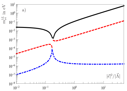
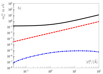
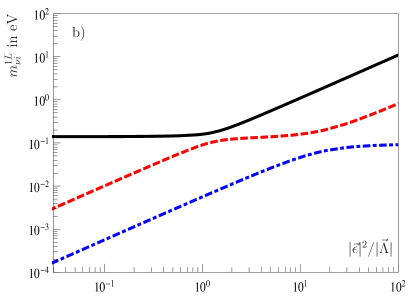
Figure 1: Three on-shell neutrino masses mνi1Lsuperscriptsubscript𝑚subscript𝜈𝑖1𝐿m_{\nu_{i}}^{1L} in eV as a function of |ϵ|2/|Λ|superscriptitalic-ϵ2Λ|\vec{\epsilon}|^{2}/|\vec{\Lambda}| for a scenario in a) the μν𝜇𝜈\mu\nuSSM based on mSUGRA 111; b) BRpV based on SPS 333.
Refer to caption
Refer to caption
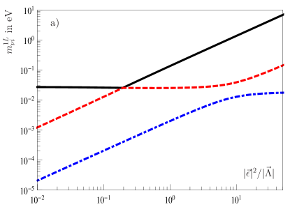
Figure 2: Three on-shell neutrino masses mνi1Lsuperscriptsubscript𝑚subscript𝜈𝑖1𝐿m_{\nu_{i}}^{1L} in eV as a function of |ϵ|2/|Λ|superscriptitalic-ϵ2Λ|\vec{\epsilon}|^{2}/|\vec{\Lambda}| using the sign-condition defined in Equation (89) for a scenario in a) μν𝜇𝜈\mu\nuSSM based on mSUGRA 111; b) BRpV based on SPS 333.

Figure 2 shows the neutrino masses mνi1Lsuperscriptsubscript𝑚subscript𝜈𝑖1𝐿m_{\nu_{i}}^{1L} of the three left-handed neutrinos as a function of |ϵ|2/|Λ|superscriptitalic-ϵ2Λ|\vec{\epsilon}|^{2}/|\vec{\Lambda}|, where we have chosen ϵ1=ϵ2=ϵ3subscriptitalic-ϵ1subscriptitalic-ϵ2subscriptitalic-ϵ3\epsilon_{1}=\epsilon_{2}=\epsilon_{3} and Λ1=Λ2=Λ3subscriptΛ1subscriptΛ2subscriptΛ3\Lambda_{1}=\Lambda_{2}=\Lambda_{3} and a fixed value of |Λ|=0.235 GeV2Λ0.235superscript GeV2|\vec{\Lambda}|=0.235\text{~{}GeV}^{2}. In case of the μν𝜇𝜈\mu\nuSSM the scenario is based on mSUGRA 111 and in case of BRpV on SPS 333. In Figure 2 we set Λ1=Λ2=Λ3subscriptΛ1subscriptΛ2subscriptΛ3\Lambda_{1}=-\Lambda_{2}=\Lambda_{3}, so that the sign-condition

ϵ2ϵ3Λ2Λ3<0subscriptitalic-ϵ2subscriptitalic-ϵ3subscriptΛ2subscriptΛ30\displaystyle\frac{\epsilon_{2}}{\epsilon_{3}}\frac{\Lambda_{2}}{\Lambda_{3}}<0 (89)

is fulfilled. This allows for a simpler fit to the solar angle, since it helps to decouple the atmospheric and the solar problem by reducing the contributions from the b𝑏b-term in the effective neutrino mass matrix at one-loop level in Equation (86) [30, 31]. We will therefore make use of the sign-condition in the following. Both models show a similar behavior.

The absolute value of |ϵ|italic-ϵ|\vec{\epsilon}| determines the neutrino masses mν11Lsuperscriptsubscript𝑚subscript𝜈11𝐿m_{\nu_{1}}^{1L} and mν21Lsuperscriptsubscript𝑚subscript𝜈21𝐿m_{\nu_{2}}^{1L}, which are generated at one-loop level, whereas the tree level neutrino mass mν31Lsuperscriptsubscript𝑚subscript𝜈31𝐿m_{\nu_{3}}^{1L} is set constant by |Λ|Λ|\vec{\Lambda}| for small |ϵ|italic-ϵ|\vec{\epsilon}| and is only affected by the one-loop corrections for large values of |ϵ|italic-ϵ|\vec{\epsilon}|. Note that for the explanation of the neutrino data the individual ϵisubscriptitalic-ϵ𝑖\epsilon_{i} and ΛisubscriptΛ𝑖\Lambda_{i} have to be chosen differently. In case of the scenarios without sign-condition a level-crossing as in Figure 2 a) can take place, which existence is dependent on the parameter point in the μν𝜇𝜈\mu\nuSSM as well as in BRpV. It corresponds to a sign-flip between mν11Lsuperscriptsubscript𝑚subscript𝜈11𝐿m_{\nu_{1}}^{1L} and mν31Lsuperscriptsubscript𝑚subscript𝜈31𝐿m_{\nu_{3}}^{1L}.

The Yukawa couplings Ylsubscript𝑌𝑙Y_{l} of the leptons at tree level have to be adopted such, that the tree level lepton masses coincide with the experimental values. Suppose we have fitted the tree level lepton masses mlsubscript𝑚𝑙m_{l} to the experimental values, we can define the relative one-loop corrections by

δl=|ml1Lmlml|.subscript𝛿𝑙subscriptsuperscript𝑚1𝐿𝑙subscript𝑚𝑙subscript𝑚𝑙\displaystyle\delta_{l}=\left|\frac{m^{1L}_{l}-m_{l}}{m_{l}}\right|\quad. (90)

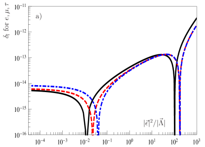
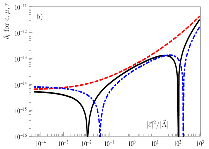
For the μν𝜇𝜈\mu\nuSSM scenarios already presented in Figures 2 a) and 2 a) with respect to the neutrino masses, Figure 3 shows the relative correction δlsubscript𝛿𝑙\delta_{l} for the lepton masses at one-loop level. For reasonable neutrino masses the corrections to the lepton masses are small δl<1010subscript𝛿𝑙superscript1010\delta_{l}<10^{-10}, even for the electron below the experimental uncertainties. Note that the shown dips correspond to a sign change, since we show the absolute value of the correction.
Refer to caption
Refer to caption
Figure 3: Corrections δlsubscript𝛿𝑙\delta_{l} defined in Equation (90) for the three lepton masses (τ𝜏\tau (black, solid), μ𝜇\mu (red, dashed), e𝑒e (blue, dot-dashed)) as a function of |ϵ|2/|Λ|superscriptitalic-ϵ2Λ|\vec{\epsilon}|^{2}/|\vec{\Lambda}| for the μν𝜇𝜈\mu\nuSSM as in Figure 2 a), in detail a) without sign-condition (89); b) with sign-condition (89).

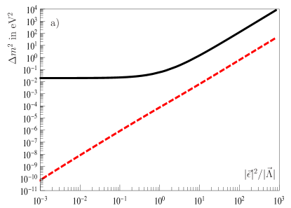
In the following we want to point out the difference between the DR¯¯DR\overline{\text{DR}} masses in [30] and the on-shell masses as defined in this article. For BRpV based on SPS 333 we present both schemes in Figure 4.

Refer to caption
Refer to caption
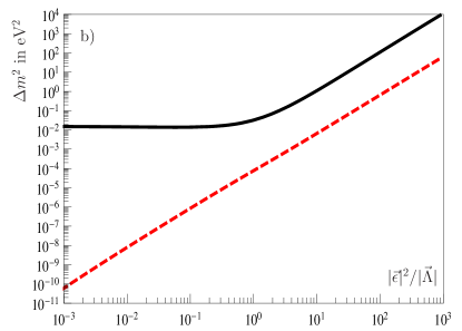
Figure 4: Mass differences Δmatm2Δsubscriptsuperscript𝑚2𝑎𝑡𝑚\Delta m^{2}_{atm} (black, solid) and Δmsol2Δsubscriptsuperscript𝑚2𝑠𝑜𝑙\Delta m^{2}_{sol} (red, dashed) as a function of |ϵ|2/|Λ|superscriptitalic-ϵ2Λ|\vec{\epsilon}|^{2}/|\vec{\Lambda}| for BRpV based on SPS 333 using the a) on-shell masses defined in Section 3; b) DR¯¯DR\overline{\text{DR}} masses as defined in [30].

Although there exists a difference in the lightest neutrino mass mν11Lsuperscriptsubscript𝑚subscript𝜈11𝐿m_{\nu_{1}}^{1L}, the mass differences Δmatm2Δsubscriptsuperscript𝑚2𝑎𝑡𝑚\Delta m^{2}_{atm} and Δmsol2Δsubscriptsuperscript𝑚2𝑠𝑜𝑙\Delta m^{2}_{sol} defined in Equation (87) are very similar, since those are given by the absolute values of mν31Lsuperscriptsubscript𝑚subscript𝜈31𝐿m_{\nu_{3}}^{1L} and mν21Lsuperscriptsubscript𝑚subscript𝜈21𝐿m_{\nu_{2}}^{1L}. Since the on-shell procedure tends to reduce the impact of the one-loop contributions, the largest mass mν31Lsuperscriptsubscript𝑚subscript𝜈31𝐿m_{\nu_{3}}^{1L} is in some scenarios only for larger values of |ϵ|italic-ϵ|\vec{\epsilon}| affected by the one-loop contributions when comparing the on-shell with the DR¯¯DR\overline{\text{DR}} masses. However, for the neutrinos the two renormalization prescriptions are very similar, whereas for the other neutralinos and charginos and in particular for the leptons the corrections are (much) smaller in case of on-shell masses compared to the DR¯¯DR\overline{\text{DR}} masses. In the scenarios above δlsubscript𝛿𝑙\delta_{l} for DR¯¯DR\overline{\text{DR}} lepton masses is between 0.30.30.3 and 222%. The one-loop corrections to the neutralino and chargino masses are included in Table 2 and are typically in the per-mil range, whereas in case of DR¯¯DR\overline{\text{DR}} masses the corrections are in the order of a few per-cent [44].

4.3 Relation between ΛΛ\vec{\Lambda}, ϵitalic-ϵ\vec{\epsilon} and the neutrino mass differences/the mixing angles

In this section we discuss the relations between the neutrino mass differences, the mixing angles and the alignment parameters ϵitalic-ϵ\vec{\epsilon} and ΛΛ\vec{\Lambda}. We refer to [10] for the current neutrino data, which we presented in Table 1. For all figures presented in this section we fit ϵitalic-ϵ\vec{\epsilon} and ΛΛ\vec{\Lambda} such, that the neutrino data bounds are fulfilled except for the angle shown in the figure.

Similar to [30] we use ΛΛ\vec{\Lambda} at tree level to explain the atmospheric mass difference and the atmospheric mixing angle, whereas ϵitalic-ϵ\vec{\epsilon} respectively ϵ~~italic-ϵ\vec{\tilde{\epsilon}} at one-loop level is used for the solar mass difference and the solar mixing angle. The latter correlation to ϵ~~italic-ϵ\vec{\tilde{\epsilon}} is more distinct than the one to ϵitalic-ϵ\vec{\epsilon}, where a prerotation with the matrix 𝒩νsubscript𝒩𝜈\mathcal{N}_{\nu} diagonalizing the tree level neutrino mass matrix mννeffsuperscriptsubscript𝑚𝜈𝜈effm_{\nu\nu}^{\rm eff} given in Equation (24) according to ϵ~=𝒩vϵ~italic-ϵsubscript𝒩𝑣italic-ϵ\vec{\tilde{\epsilon}}=\mathcal{N}_{v}\vec{\epsilon} was performed. The mixing matrix 𝒩νsubscript𝒩𝜈\mathcal{N}_{\nu} is in the considered scenarios exactly given by [65]

𝒩ν=(Λ22+Λ32|Λ|Λ1Λ2Λ22+Λ32|Λ|Λ1Λ3Λ22+Λ32|Λ|0Λ3Λ22+Λ32Λ2Λ22+Λ32Λ1|Λ|Λ2|Λ|Λ3|Λ|).subscript𝒩𝜈matrixsuperscriptsubscriptΛ22superscriptsubscriptΛ32ΛsubscriptΛ1subscriptΛ2superscriptsubscriptΛ22superscriptsubscriptΛ32ΛsubscriptΛ1subscriptΛ3superscriptsubscriptΛ22superscriptsubscriptΛ32Λ0subscriptΛ3superscriptsubscriptΛ22superscriptsubscriptΛ32subscriptΛ2superscriptsubscriptΛ22superscriptsubscriptΛ32subscriptΛ1ΛsubscriptΛ2ΛsubscriptΛ3Λ\displaystyle\mathcal{N}_{\nu}=\begin{pmatrix}\frac{\sqrt{\Lambda_{2}^{2}+\Lambda_{3}^{2}}}{|\vec{\Lambda}|}&-\frac{\Lambda_{1}\Lambda_{2}}{\sqrt{\Lambda_{2}^{2}+\Lambda_{3}^{2}}|\vec{\Lambda}|}&-\frac{\Lambda_{1}\Lambda_{3}}{\sqrt{\Lambda_{2}^{2}+\Lambda_{3}^{2}}|\vec{\Lambda}|}\\ 0&\frac{\Lambda_{3}}{\sqrt{\Lambda_{2}^{2}+\Lambda_{3}^{2}}}&-\frac{\Lambda_{2}}{\sqrt{\Lambda_{2}^{2}+\Lambda_{3}^{2}}}\\ \frac{\Lambda_{1}}{|\vec{\Lambda}|}&\frac{\Lambda_{2}}{|\vec{\Lambda}|}&\frac{\Lambda_{3}}{|\vec{\Lambda}|}\end{pmatrix}\quad. (91)

We will first comment on the atmospheric and solar mass differences Δmatm2Δsubscriptsuperscript𝑚2𝑎𝑡𝑚\Delta m^{2}_{atm} and Δmsol2Δsubscriptsuperscript𝑚2𝑠𝑜𝑙\Delta m^{2}_{sol}. Whereas the atmospheric mass difference is determined by |Λ|Λ|\vec{\Lambda}|, the solar mass difference correlates with |ϵ|italic-ϵ|\vec{\epsilon}|. Therein the absolute value of ΛΛ\vec{\Lambda} can be estimated using Equation (29).
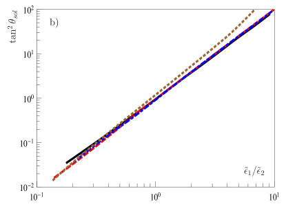
Refer to caption
Refer to caption
Figure 5: Correlation between the alignment parameters and the neutrino mixing angles for the μν𝜇𝜈\mu\nuSSM based on mSUGRA 111 (black), 3superscript33^{\prime} (red, dashed), 4superscript44^{\prime} (blue, dot-dashed) and GMSB 555 (brown, dotted) presented in Table 2, in detail a) tan2θatmsuperscript2subscript𝜃𝑎𝑡𝑚\tan^{2}\theta_{atm} as a function of Λ2/Λ3subscriptΛ2subscriptΛ3\Lambda_{2}/\Lambda_{3}; b) tan2θsolsuperscript2subscript𝜃𝑠𝑜𝑙\tan^{2}\theta_{sol} as a function of ϵ~1/ϵ~2subscript~italic-ϵ1subscript~italic-ϵ2\tilde{\epsilon}_{1}/\tilde{\epsilon}_{2}.

Using the definitions of Equation (88) for the neutrino mixing angles we will now focus on the correlation between the alignment parameters ΛisubscriptΛ𝑖\Lambda_{i} and ϵ~isubscript~italic-ϵ𝑖\tilde{\epsilon}_{i} and the neutrino mixing angles, which is shown in Figure 5. The ratio Λ2/Λ3subscriptΛ2subscriptΛ3\Lambda_{2}/\Lambda_{3} defines the atmospheric angle and ϵ~1/ϵ~2subscript~italic-ϵ1subscript~italic-ϵ2\tilde{\epsilon}_{1}/\tilde{\epsilon}_{2} fits the solar angle. The reactor angle is determined by Λ1/Λ22+Λ32subscriptΛ1superscriptsubscriptΛ22superscriptsubscriptΛ32\Lambda_{1}/\sqrt{\Lambda_{2}^{2}+\Lambda_{3}^{2}} [30] which however can receive sizable loop corrections.

5 Tree level decay widths of χ~10l±Wsuperscriptsubscript~𝜒10superscript𝑙plus-or-minussuperscript𝑊minus-or-plus\tilde{\chi}_{1}^{0}\rightarrow l^{\pm}W^{\mp}

After having discussed the finite mass corrections between tree level and one-loop level, which allow to explain the full neutrino spectrum, we will now turn to the decays χ~10l±Wsuperscriptsubscript~𝜒10superscript𝑙plus-or-minussuperscript𝑊minus-or-plus\tilde{\chi}_{1}^{0}\rightarrow l^{\pm}W^{\mp} in order to study the correlations between neutrino mixing angles and the different leptonic final states. The partial widths for the decays χ~j0χ~l±Wsuperscriptsubscript~𝜒𝑗0superscriptsubscript~𝜒𝑙plus-or-minussuperscript𝑊minus-or-plus\tilde{\chi}_{j}^{0}\rightarrow\tilde{\chi}_{l}^{\pm}W^{\mp} including the Rp/R_{p}/\;\>\hskip 1.99997ptdecays χ~10ll±Wsuperscriptsubscript~𝜒10superscriptsubscript𝑙𝑙plus-or-minussuperscript𝑊minus-or-plus\tilde{\chi}_{1}^{0}\rightarrow l_{l}^{\pm}W^{\mp} are obtained from the following interaction Lagrangian

=χ~l¯γμ(PLOLlj+PRORlj)χ~j0Wμ+h.c..formulae-sequence¯superscriptsubscript~𝜒𝑙superscript𝛾𝜇subscript𝑃𝐿subscript𝑂𝐿𝑙𝑗subscript𝑃𝑅subscript𝑂𝑅𝑙𝑗superscriptsubscript~𝜒𝑗0subscriptsuperscript𝑊𝜇𝑐\displaystyle\mathcal{L}=\overline{\tilde{\chi}_{l}^{-}}\gamma^{\mu}\left(P_{L}O_{Llj}+P_{R}O_{Rlj}\right)\tilde{\chi}_{j}^{0}W^{-}_{\mu}+h.c.\qquad. (92)

The couplings are given by

OLljsubscript𝑂𝐿𝑙𝑗\displaystyle O_{Llj} =g𝒩j2Ul112g(𝒩j3Ul2+k=13Ul,2+k𝒩j,4(5)+k)absent𝑔subscriptsuperscript𝒩𝑗2subscript𝑈𝑙112𝑔subscriptsuperscript𝒩𝑗3subscript𝑈𝑙2superscriptsubscript𝑘13subscript𝑈𝑙2𝑘superscriptsubscript𝒩𝑗45𝑘\displaystyle=-g\mathcal{N}^{*}_{j2}U_{l1}-\frac{1}{\sqrt{2}}g\left(\mathcal{N}^{*}_{j3}U_{l2}+\sum_{k=1}^{3}U_{l,2+k}\mathcal{N}_{j,4(5)+k}^{*}\right) (93)
ORljsubscript𝑂𝑅𝑙𝑗\displaystyle O_{Rlj} =gVl1𝒩j2+12gVl2𝒩j4,absent𝑔superscriptsubscript𝑉𝑙1subscript𝒩𝑗212𝑔superscriptsubscript𝑉𝑙2subscript𝒩𝑗4\displaystyle=-gV_{l1}^{*}\mathcal{N}_{j2}+\frac{1}{\sqrt{2}}gV_{l2}^{*}\mathcal{N}_{j4}\quad, (94)

where in Equation (93) the index is 444 (5)5(5) in case of BRpV (μν𝜇𝜈\mu\nuSSM). The widths have the form

Γ0=116πmi3κ(mi2,mo2,mW2)12pol|MT|2,superscriptΓ0116𝜋superscriptsubscript𝑚𝑖3𝜅superscriptsubscript𝑚𝑖2superscriptsubscript𝑚𝑜2superscriptsubscript𝑚𝑊212subscript𝑝𝑜𝑙superscriptsubscript𝑀𝑇2\Gamma^{0}=\frac{1}{16\pi m_{i}^{3}}\sqrt{\kappa(m_{i}^{2},m_{o}^{2},m_{W}^{2})}\frac{1}{2}\sum_{pol}|M_{T}|^{2}\qquad, (95)

where misubscript𝑚𝑖m_{i} (mosubscript𝑚𝑜m_{o}) is the mass of the mother (daughter) particle and MTsubscript𝑀𝑇M_{T} is the tree level matrix element. Explicitly they are given by

Γ0(χ~j0χ~l+W)=superscriptΓ0superscriptsubscript~𝜒𝑗0superscriptsubscript~𝜒𝑙superscript𝑊absent\displaystyle\Gamma^{\mathrm{0}}\left(\tilde{\chi}_{j}^{0}\rightarrow\tilde{\chi}_{l}^{+}W^{-}\right)= 116πmj3κ(mj2,ml2,mW2)116𝜋superscriptsubscript𝑚𝑗3𝜅superscriptsubscript𝑚𝑗2superscriptsubscript𝑚𝑙2superscriptsubscript𝑚𝑊2\displaystyle\frac{1}{16\pi m_{j}^{3}}\sqrt{\kappa(m_{j}^{2},m_{l}^{2},m_{W}^{2})}
×((|OLlj|2+\displaystyle\times\Big{(}\big{(}|O_{Llj}|^{2}+ |ORlj|2)f(mj2,ml2,mW2)6Re(OLljORlj)mjml)\displaystyle|O_{Rlj}|^{2}\big{)}f(m_{j}^{2},m_{l}^{2},m_{W}^{2})-6\mathrm{Re}(O_{Llj}O_{Rlj}^{*})m_{j}m_{l}\Big{)} (96)
Γ0(χ~i+χ~k0W+)=superscriptΓ0superscriptsubscript~𝜒𝑖superscriptsubscript~𝜒𝑘0superscript𝑊absent\displaystyle\Gamma^{\mathrm{0}}\left(\tilde{\chi}_{i}^{+}\rightarrow\tilde{\chi}_{k}^{0}W^{+}\right)= 116πmi3κ(mi2,mk2,mW2)116𝜋superscriptsubscript𝑚𝑖3𝜅superscriptsubscript𝑚𝑖2superscriptsubscript𝑚𝑘2superscriptsubscript𝑚𝑊2\displaystyle\frac{1}{16\pi m_{i}^{3}}\sqrt{\kappa(m_{i}^{2},m_{k}^{2},m_{W}^{2})}
×((|OLik|2+\displaystyle\times\Big{(}\big{(}|O_{Lik}|^{2}+ |ORik|2)f(mi2,mk2,mW2)6Re(OLikORik)mimk)\displaystyle|O_{Rik}|^{2}\big{)}f(m_{i}^{2},m_{k}^{2},m_{W}^{2})-6\mathrm{Re}(O_{Lik}O_{Rik}^{*})m_{i}m_{k}\Big{)} (97)

using the functions

f(x,y,z)=𝑓𝑥𝑦𝑧absent\displaystyle f(x,y,z)= 12(x+y)z+(xy)22z12𝑥𝑦𝑧superscript𝑥𝑦22𝑧\displaystyle\frac{1}{2}(x+y)-z+\frac{(x-y)^{2}}{2z} (98)
κ(x,y,z)=𝜅𝑥𝑦𝑧absent\displaystyle\kappa(x,y,z)= x2+y2+z22xy2xz2yz.superscript𝑥2superscript𝑦2superscript𝑧22𝑥𝑦2𝑥𝑧2𝑦𝑧\displaystyle x^{2}+y^{2}+z^{2}-2xy-2xz-2yz\qquad. (99)

Coupling χ~10liW±superscriptsubscript~𝜒10subscriptsuperscript𝑙minus-or-plus𝑖superscript𝑊plus-or-minus\tilde{\chi}_{1}^{0}-l^{\mp}_{i}-W^{\pm}

The tree level couplings OLi1subscript𝑂𝐿𝑖1O_{Li1} in Equation (93) and ORi1subscript𝑂𝑅𝑖1O_{Ri1} in Equation (94) for the special case of the lightest neutralino χ~10superscriptsubscript~𝜒10\tilde{\chi}_{1}^{0} coupling to a lepton lisubscript𝑙𝑖l_{i} can be approximated in terms of the alignment parameters ΛisubscriptΛ𝑖\Lambda_{i} and ϵisubscriptitalic-ϵ𝑖\epsilon_{i}, which allows to understand the correlations to the neutrino mixing angles. Although we have shown these approximated couplings in great detail already in [47] for the μν𝜇𝜈\mu\nuSSM, their knowledge is of great importance. The right-handed couplings ORi1subscript𝑂𝑅𝑖1O_{Ri1} can be approximated in BRpV and the μν𝜇𝜈\mu\nuSSM by:

ORi1subscript𝑂𝑅𝑖1\displaystyle O_{Ri1} g(Yl)iivd2Det+[gvuN12M2N14μϵi+g(2μ2+g2vu2)N12g2(vdμ+M2vu)N142μDet+Λi]absent𝑔subscriptsubscript𝑌𝑙𝑖𝑖subscript𝑣𝑑2Desubscripttdelimited-[]𝑔subscript𝑣𝑢subscript𝑁12subscript𝑀2subscript𝑁14𝜇subscriptitalic-ϵ𝑖𝑔2superscript𝜇2superscript𝑔2superscriptsubscript𝑣𝑢2subscript𝑁12superscript𝑔2subscript𝑣𝑑𝜇subscript𝑀2subscript𝑣𝑢subscript𝑁142𝜇subscriptDetsubscriptΛ𝑖\displaystyle\approx\frac{g(Y_{l})_{ii}v_{d}}{2\mathrm{Det}_{+}}\left[\frac{gv_{u}N_{12}-M_{2}N_{14}}{\mu}\epsilon_{i}+\frac{g(2\mu^{2}+g^{2}v_{u}^{2})N_{12}-g^{2}(v_{d}\mu+M_{2}v_{u})N_{14}}{2\mu\mathrm{Det}_{+}}\Lambda_{i}\right] (100)

Therein the determinant of the heavy states in the chargino mass matrix appears

Det+subscriptDet\displaystyle\mathrm{Det}_{+} =M2μ12g2vdvu.absentsubscript𝑀2𝜇12superscript𝑔2subscript𝑣𝑑subscript𝑣𝑢\displaystyle=M_{2}\mu-\frac{1}{2}g^{2}v_{d}v_{u}\quad. (101)

In contrast the left-handed couplings differ in both models and are given by the following expressions:

OLi1bRp/\displaystyle O_{Li1}^{b\text{$R_{p}/\;\>\hskip 1.39998pt$}}\approx gΛi2[gM2μ2Det0bRp/N11+(gDet++gM1μ2Det0bRp/)N12\displaystyle\frac{g\Lambda_{i}}{\sqrt{2}}\left[-\frac{g^{\prime}M_{2}\mu}{2\mathrm{Det}_{0}^{b\text{$R_{p}/\;\>\hskip 1.39998pt$}}}N_{11}+\left(\frac{g}{\mathrm{Det}_{+}}+\frac{gM_{1}\mu}{2\mathrm{Det}_{0}^{b\text{$R_{p}/\;\>\hskip 1.39998pt$}}}\right)N_{12}\right.
vu2(mγ2Det0bRp/+g2μDet+)N13+vdmγ4Det0bRp/N14]\displaystyle\qquad-\frac{v_{u}}{2}\left(\frac{m_{\gamma}}{2\mathrm{Det}_{0}^{b\text{$R_{p}/\;\>\hskip 1.39998pt$}}}+\frac{g^{2}}{\mu\mathrm{Det}_{+}}\right)N_{13}+\left.\frac{v_{d}m_{\gamma}}{4\mathrm{Det}_{0}^{b\text{$R_{p}/\;\>\hskip 1.39998pt$}}}N_{14}\right] (102)
OLi1μνSSMsuperscriptsubscript𝑂𝐿𝑖1𝜇𝜈SSMabsent\displaystyle O_{Li1}^{\mu\nu\text{SSM}}\approx gΛi2[gM22Det0μνSSM(vdvuλ2+mRμ)N11\displaystyle\frac{g\Lambda_{i}}{\sqrt{2}}\left[-\frac{g^{\prime}M_{2}}{2\mathrm{Det}_{0}^{\mu\nu\text{SSM}}}(v_{d}v_{u}\lambda^{2}+m_{R}\mu)N_{11}\right.
+(gDet++gM12Det0μνSSM(vdvuλ2+mRμ))N12𝑔subscriptDet𝑔subscript𝑀12Desuperscriptsubscriptt0𝜇𝜈SSMsubscript𝑣𝑑subscript𝑣𝑢superscript𝜆2subscript𝑚𝑅𝜇subscript𝑁12\displaystyle\qquad+\left(\frac{g}{\mathrm{Det}_{+}}+\frac{gM_{1}}{2\mathrm{Det}_{0}^{\mu\nu\text{SSM}}}(v_{d}v_{u}\lambda^{2}+m_{R}\mu)\right)N_{12}
(g2vu2μDet+mγ8μDet0μνSSM(λ2vd(vd2+vu2)+2mRμvu))N13superscript𝑔2subscript𝑣𝑢2𝜇subscriptDetsubscript𝑚𝛾8𝜇superscriptsubscriptDet0𝜇𝜈SSMsuperscript𝜆2subscript𝑣𝑑superscriptsubscript𝑣𝑑2superscriptsubscript𝑣𝑢22subscript𝑚𝑅𝜇subscript𝑣𝑢subscript𝑁13\displaystyle\qquad-\left(\frac{g^{2}v_{u}}{2\mu\mathrm{Det}_{+}}-\frac{m_{\gamma}}{8\mu\mathrm{Det}_{0}^{\mu\nu\text{SSM}}}(\lambda^{2}v_{d}(v_{d}^{2}+v_{u}^{2})+2m_{R}\mu v_{u})\right)N_{13}
+mγ8μDet0μνSSM(λ2vu(vd2+vu2)+2mRμvd)N14subscript𝑚𝛾8𝜇superscriptsubscriptDet0𝜇𝜈SSMsuperscript𝜆2subscript𝑣𝑢superscriptsubscript𝑣𝑑2superscriptsubscript𝑣𝑢22subscript𝑚𝑅𝜇subscript𝑣𝑑subscript𝑁14\displaystyle\qquad+\frac{m_{\gamma}}{8\mu\mathrm{Det}_{0}^{\mu\nu\text{SSM}}}(\lambda^{2}v_{u}(v_{d}^{2}+v_{u}^{2})+2m_{R}\mu v_{d})N_{14}
λmγ42Det0μνSSM(vu2vd2)N15]\displaystyle\qquad\left.-\frac{\lambda m_{\gamma}}{4\sqrt{2}\mathrm{Det}_{0}^{\mu\nu\text{SSM}}}(v_{u}^{2}-v_{d}^{2})N_{15}\right] (103)

The couplings include the abbreviations of Equations (8),(9) and (26) and the determinants shown in Equations (27) and (28). Neglecting the right-handed couplings, which are generally smaller than the left-handed ones, it is obvious that the lightest neutralino χ~10superscriptsubscript~𝜒10\tilde{\chi}_{1}^{0} couples to li±Wsuperscriptsubscript𝑙𝑖plus-or-minussuperscript𝑊minus-or-plusl_{i}^{\pm}W^{\mp} proportional to ΛisubscriptΛ𝑖\Lambda_{i} without any dependence on the ϵisubscriptitalic-ϵ𝑖\epsilon_{i} parameters. This fact is in case of the considered BRpV and the μν𝜇𝜈\mu\nuSSM independent of the nature of the lightest neutralino χ~10superscriptsubscript~𝜒10\tilde{\chi}_{1}^{0}. However, it is important to emphasize that all previous formulas are tree level results. A priori it is not clear, what happens if one uses the mixing matrices 𝒩𝒩\mathcal{N}, U𝑈U and V𝑉V for masses at one-loop level or performs a complete NLO calculation of the decay width.

6 NLO decay widths of χ~10l±Wsuperscriptsubscript~𝜒10superscript𝑙plus-or-minussuperscript𝑊minus-or-plus\tilde{\chi}_{1}^{0}\rightarrow l^{\pm}W^{\mp} and correlations to neutrino mixing angles

In this section we focus on the NLO decay widths Γ1(χ~10l+W)superscriptΓ1superscriptsubscript~𝜒10superscript𝑙superscript𝑊\Gamma^{1}\left(\tilde{\chi}_{1}^{0}\rightarrow l^{+}W^{-}\right). The calculation procedure was introduced in [45] and can be adopted for BRpV and the μν𝜇𝜈\mu\nuSSM without any changes. The corresponding formulas have been implemented in the public program CNNDecays [51]. All technical questions concerning the used renormalization scheme like the cancellation of UV and IR divergences or gauge invariance have been discussed in [45] for the (N)MSSM and preserve their validity for the R𝑅R-parity violating extensions.

6.1 Absolute size of the corrections

In Figure 6 we present the NLO decay width for a mSUGRA 444 based scenario, where we varied κ=0.10.5𝜅0.10.5\kappa=0.1-0.5 in order to have a singlino- and a higgsino-like lightest neutralino χ~10superscriptsubscript~𝜒10\tilde{\chi}_{1}^{0} in comparison. For κ0.1less-than-or-similar-to𝜅0.1\kappa\lesssim 0.1 the decay is near the kinematical threshold and for κ0.5much-greater-than𝜅0.5\kappa\gg 0.5 a Landau pole appears. We show the relative correction δ(χ~10l+W)𝛿superscriptsubscript~𝜒10superscript𝑙superscript𝑊\delta(\tilde{\chi}_{1}^{0}\rightarrow l^{+}W^{-}), which is defined by:

δ(χ~10l+W)=Γ1(χ~10l+W)Γ0(χ~10l+W)Γ0(χ~10l+W)𝛿superscriptsubscript~𝜒10superscript𝑙superscript𝑊superscriptΓ1superscriptsubscript~𝜒10superscript𝑙superscript𝑊superscriptΓ0superscriptsubscript~𝜒10superscript𝑙superscript𝑊superscriptΓ0superscriptsubscript~𝜒10superscript𝑙superscript𝑊\displaystyle\delta(\tilde{\chi}_{1}^{0}\rightarrow l^{+}W^{-})=\frac{\Gamma^{1}(\tilde{\chi}_{1}^{0}\rightarrow l^{+}W^{-})-\Gamma^{0}(\tilde{\chi}_{1}^{0}\rightarrow l^{+}W^{-})}{\Gamma^{0}(\tilde{\chi}_{1}^{0}\rightarrow l^{+}W^{-})} (104)

The size and the sign of the corrections is strongly dependent on the size and the sign of the R𝑅R-parity violating parameters visubscript𝑣𝑖v_{i} and Yνisuperscriptsubscript𝑌𝜈𝑖Y_{\nu}^{i} or ΛisubscriptΛ𝑖\Lambda_{i} and ϵisubscriptitalic-ϵ𝑖\epsilon_{i}. In Figure 6 we set Λ=(0.31,5.21,2.02)102Λ0.315.212.02superscript102\vec{\Lambda}=(0.31,5.21,2.02)\cdot 10^{-2} GeV2 and ϵ=(7.49,9.61,6.57)103italic-ϵ7.499.616.57superscript103\vec{\epsilon}=(7.49,9.61,-6.57)\cdot 10^{-3} GeV. Since the solar mass difference and mixing angle are only well defined at one-loop level, the corrections to the decay χ~10e+Wsuperscriptsubscript~𝜒10superscript𝑒superscript𝑊\tilde{\chi}_{1}^{0}\rightarrow e^{+}W^{-} are sizable and can be of the order of the tree level decay width or larger. The corrections to χ~10μ+Wsuperscriptsubscript~𝜒10superscript𝜇superscript𝑊\tilde{\chi}_{1}^{0}\rightarrow\mu^{+}W^{-} or τ+Wsuperscript𝜏superscript𝑊\tau^{+}W^{-} are generally smaller, but remain of order 10%percent1010\%.

Refer to caption
Refer to caption
Refer to caption
Refer to caption
Figure 6: Neutralino masses, particle content of the lightest neutralino and decay widths Γ1(χ~10l+W)superscriptΓ1superscriptsubscript~𝜒10superscript𝑙superscript𝑊\Gamma^{1}(\tilde{\chi}_{1}^{0}\rightarrow l^{+}W^{-}) as a function of κ𝜅\kappa within the μν𝜇𝜈\mu\nuSSM based on the mSUGRA 444 scenario and Λ=(0.31,5.21,2.02)102Λ0.315.212.02superscript102\vec{\Lambda}=(0.31,5.21,2.02)\cdot 10^{-2} GeV2 and ϵ=(7.49,9.61,6.57)103italic-ϵ7.499.616.57superscript103\vec{\epsilon}=(7.49,9.61,-6.57)\cdot 10^{-3} GeV: a) Neutralino masses mχ~i01Lsuperscriptsubscript𝑚superscriptsubscript~𝜒𝑖01𝐿m_{\tilde{\chi}_{i}^{0}}^{1L} (mχ~101Lsuperscriptsubscript𝑚superscriptsubscript~𝜒101𝐿m_{\tilde{\chi}_{1}^{0}}^{1L} (red, solid), mχ~2,3,401Lsuperscriptsubscript𝑚superscriptsubscript~𝜒23401𝐿m_{\tilde{\chi}_{2,3,4}^{0}}^{1L} (black, dashed)); b) Particle character |𝒩4i1L|2superscriptsuperscriptsubscript𝒩4𝑖1𝐿2|\mathcal{N}_{4i}^{1L}|^{2} (ν~csuperscript~𝜈𝑐\tilde{\nu}^{c} (red, solid), H~u+H~dsubscript~𝐻𝑢subscript~𝐻𝑑\tilde{H}_{u}+\tilde{H}_{d} (blue, dashed), B~~𝐵\tilde{B} (black, dot-dashed), W~~𝑊\tilde{W} (orange, dot-dashed)); c) NLO decay width Γ1superscriptΓ1\Gamma^{1} (e𝑒e (blue, dot-dashed), μ𝜇\mu (red, dashed), τ𝜏\tau (black)); d) Relative correction δ𝛿\delta defined in Equation (104) (e𝑒e (blue, dot-dashed), μ𝜇\mu (red, dashed), τ𝜏\tau (black)).

6.2 Correlation between decay widths and neutrino mixing angles

Having discussed the absolute size of the NLO contributions to the decay widths of the two body decays χ~10l+Wsuperscriptsubscript~𝜒10superscript𝑙superscript𝑊\tilde{\chi}_{1}^{0}\rightarrow l^{+}W^{-}, we will now focus on the correlations between the branching ratios and the neutrino mixing angles. We have shown in Section 5, that the tree level couplings can be approximated in terms of the alignment parameters ΛΛ\vec{\Lambda} and ϵitalic-ϵ\vec{\epsilon}. Since the alignment parameters are connected to the neutrino mixing angles as explained in Section 4.3, one can expect the following tree level relation:

Γ0(χ~10μ+W)Γ0(χ~10τ+W)(OL21OL31)2(Λ2Λ3)2tan2θatmproportional-tosuperscriptΓ0superscriptsubscript~𝜒10superscript𝜇superscript𝑊superscriptΓ0superscriptsubscript~𝜒10superscript𝜏superscript𝑊superscriptsubscript𝑂𝐿21subscript𝑂𝐿312superscriptsubscriptΛ2subscriptΛ32superscript2subscript𝜃𝑎𝑡𝑚\displaystyle\frac{\Gamma^{0}(\tilde{\chi}_{1}^{0}\rightarrow\mu^{+}W^{-})}{\Gamma^{0}(\tilde{\chi}_{1}^{0}\rightarrow\tau^{+}W^{-})}\propto\left(\frac{O_{L21}}{O_{L31}}\right)^{2}\approx\left(\frac{\Lambda_{2}}{\Lambda_{3}}\right)^{2}\approx\tan^{2}\theta_{atm} (105)

It is a priori not clear to which extent this relation also holds at one-loop level. We have found that using one-loop corrected DR¯¯DR\overline{\text{DR}} masses together with the corresponding one-loop corrected mixing matrix 𝒩1Lsuperscript𝒩1𝐿\mathcal{N}^{1L} in the tree level decay width can spoil this relation. However, performing the full one-loop corrections including the real corrections from photon emission in the considered on-shell scheme retains the predictions at tree level, so that

Γ1(χ~10μ+W)Γ1(χ~10τ+W)(Λ2Λ3)2tan2θatm.proportional-tosuperscriptΓ1superscriptsubscript~𝜒10superscript𝜇superscript𝑊superscriptΓ1superscriptsubscript~𝜒10superscript𝜏superscript𝑊superscriptsubscriptΛ2subscriptΛ32superscript2subscript𝜃𝑎𝑡𝑚\displaystyle\frac{\Gamma^{1}(\tilde{\chi}_{1}^{0}\rightarrow\mu^{+}W^{-})}{\Gamma^{1}(\tilde{\chi}_{1}^{0}\rightarrow\tau^{+}W^{-})}\propto\left(\frac{\Lambda_{2}}{\Lambda_{3}}\right)^{2}\approx\tan^{2}\theta_{atm}\quad. (106)

In Figure 7 we highlight this feature using the scenarios of Table 2 for the μν𝜇𝜈\mu\nuSSM. We do not only show the tree level and one-loop relations, but also the relations obtained by using the one-loop mixing matrices 𝒩1L,U1Lsuperscript𝒩1𝐿superscript𝑈1𝐿\mathcal{N}^{1L},U^{1L} and V1Lsuperscript𝑉1𝐿V^{1L} within the tree level decay width Γ0(χ~10l+W)superscriptΓ0superscriptsubscript~𝜒10superscript𝑙superscript𝑊\Gamma^{0}(\tilde{\chi}_{1}^{0}\rightarrow l^{+}W^{-}), see Equation (5). The ratios are shown as a function of Λ2/Λ3subscriptΛ2subscriptΛ3\Lambda_{2}/\Lambda_{3}, which is equivalent to varying tan2θatmsuperscript2subscript𝜃𝑎𝑡𝑚\tan^{2}\theta_{atm} as can be seen in Figure 5. We vary the other parameters such, that the neutrino data are within their 2σ2𝜎2\sigma bounds as given in Table 1. This is the cause of the observed widths in case of the mSUGRA 4superscript44^{\prime} scenario.

Refer to caption
Refer to caption
Refer to caption
Refer to caption
Figure 7: Ratios Γ(χ~10μ+W)/Γ(χ~10τ+W)Γsuperscriptsubscript~𝜒10superscript𝜇superscript𝑊Γsuperscriptsubscript~𝜒10superscript𝜏superscript𝑊\Gamma(\tilde{\chi}_{1}^{0}\rightarrow\mu^{+}W^{-})/\Gamma(\tilde{\chi}_{1}^{0}\rightarrow\tau^{+}W^{-}) with Γ=Γ0ΓsuperscriptΓ0\Gamma=\Gamma^{0} in black, Γ=Γ1ΓsuperscriptΓ1\Gamma=\Gamma^{1} in red, dashed, Γ=Γ0ΓsuperscriptΓ0\Gamma=\Gamma^{0} with 𝒩1Lsuperscript𝒩1𝐿\mathcal{N}^{1L} in blue, dot-dashed, Γ=Γ0ΓsuperscriptΓ0\Gamma=\Gamma^{0} with 𝒩1L,U1Lsuperscript𝒩1𝐿superscript𝑈1𝐿\mathcal{N}^{1L},U^{1L} and V1Lsuperscript𝑉1𝐿V^{1L} in brown, dotted as a function of Λ2/Λ3subscriptΛ2subscriptΛ3\Lambda_{2}/\Lambda_{3} for the μν𝜇𝜈\mu\nuSSM scenarios of Table 2: a) mSUGRA 111; b) mSUGRA 3superscript33^{\prime}; c) mSUGRA 4superscript44^{\prime}; d) GMSB 555.

As already known from BRpV the approximated one-loop contributions using Γ0superscriptΓ0\Gamma^{0} together with the one-loop corrected mixing matrices show the expected behavior if the lightest neutralino is either mainly a bino, wino or a pure higgsino. However, in case that the singlino-component gets sizable or dominant, these approximations fail and the complete one-loop decay width Γ1superscriptΓ1\Gamma^{1} has to be calculated to obtain a reliable result. In case of mSUGRA 4superscript44^{\prime}, which is shown in Figure 7, the higgsino has a purity of 91.7%percent91.791.7\%, but a singlino component of 6.9%percent6.96.9\% is left, so that also in this case the full one-loop decay width is advisable.

The reason for the misleading ratios in case of a singlino-like neutralino is a cancellation between the second and the last terms of the left-handed coupling OLl1subscript𝑂𝐿𝑙1O_{Ll1} in Equation (93) at tree level. Replacing the tree level mixing matrix 𝒩𝒩\mathcal{N} by the one-loop mixing matrix 𝒩1Lsuperscript𝒩1𝐿\mathcal{N}^{1L} spoils this cancellation, so that unreasonable results for the decay widths and also the ratios are obtained. However, the very same effect is restored once the complete one-loop corrections are included.

For completeness let us briefly discuss the situation within BRpV. As examples we take scenarios where the lightest neutralino is either mainly a bino, scenario SPS 333, or mainly a higgsino, scenario SPS 2superscript22^{\prime}. The ratios of decay widths using the various approximations are shown in Figure 8. We observe that NLO corrections are somewhat more important for higgsino-like neutralinos: Here the combination of tree level decay widths with NLO masses and mixing matrices can lead to correlations which are off by a factor 2 compared the case of the complete NLO calculation. Moreover, the complete NLO corrections can shift the correlations up to 30 per-cent compared to the tree level result.
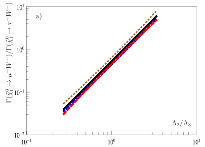
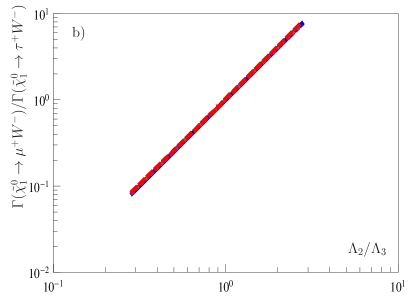
Refer to caption
Refer to caption
Figure 8: Ratios Γ(χ~10μ+W)/Γ(χ~10τ+W)Γsuperscriptsubscript~𝜒10superscript𝜇superscript𝑊Γsuperscriptsubscript~𝜒10superscript𝜏superscript𝑊\Gamma(\tilde{\chi}_{1}^{0}\rightarrow\mu^{+}W^{-})/\Gamma(\tilde{\chi}_{1}^{0}\rightarrow\tau^{+}W^{-}) with Γ=Γ0ΓsuperscriptΓ0\Gamma=\Gamma^{0} in black, Γ=Γ1ΓsuperscriptΓ1\Gamma=\Gamma^{1} in red, dashed, Γ=Γ0ΓsuperscriptΓ0\Gamma=\Gamma^{0} with 𝒩1Lsuperscript𝒩1𝐿\mathcal{N}^{1L} in blue, dot-dashed, Γ=Γ0ΓsuperscriptΓ0\Gamma=\Gamma^{0} with 𝒩1L,U1Lsuperscript𝒩1𝐿superscript𝑈1𝐿\mathcal{N}^{1L},U^{1L} and V1Lsuperscript𝑉1𝐿V^{1L} in brown, dotted as a function of Λ2/Λ3subscriptΛ2subscriptΛ3\Lambda_{2}/\Lambda_{3} for the BRpV scenarios of Table 2: a) SPS 2superscript22^{\prime}; b) SPS 333.

7 Conclusion

In Rp/R_{p}/\;\>\hskip 1.99997ptmodels, where the sneutrinos obtain a VEV, a mixing between charged leptons and charginos as well as a mixing between neutrinos and neutralinos occur at tree level. The latter can be used to obtain at least one neutrino mass at tree level. The other neutrino masses can be generated at the one-loop level as it happens e.g. in bilinear Rp/R_{p}/\;\>\hskip 1.99997ptor in the μν𝜇𝜈\mu\nuSSM with one generation of right-handed neutrinos. In previous work a DR¯¯DR\overline{\text{DR}} scheme had been used for this. In this paper we worked out an on-shell scheme and compared both schemes. The challenge here is, that there are less parameters than masses implying finite shifts at the one-loop level to the masses. With respect to the masses of neutrinos and charged leptons we have found only small differences well below the current and near future experimental accuracies.

In both models one expects correlations between ratios of the decay widths or equivalently the branching ratios for the decays χ~10l±Wsubscriptsuperscript~𝜒01superscript𝑙plus-or-minussuperscript𝑊minus-or-plus\tilde{\chi}^{0}_{1}\rightarrow l^{\pm}W^{\mp} and the atmospheric mixing angle which can be shown easily at tree level using approximate formulas for the mixing matrices. We have calculated these decays including the complete NLO order corrections in the on-shell scheme and compared the results to the pure tree level as well as to the case where one uses tree level formulas for the decay widths but one-loop corrected masses and mixing matrices.

We have found that corrections to the channels containing either a μ𝜇\mu or a τ𝜏\tau lepton are typically of order ten per-cent whereas the corrections for the e𝑒e-channel can be of the order of the tree level decay width. The reason for the latter finding is that the solar mixing angle is not well defined at tree level but only at the one-loop level. For the correlations between the decay widths and the atmospheric mixing angle we find that in case of gaugino-like neutralino in all approximations nearly the same correlations. However, already for doublet-higgsino-like neutralino the correlations can be off by a factor two if one combines tree level widths with one-loop corrected masses and mixing angles. In case of a neutralino which has either a sizable singlino-component or which is dominantly singlino-like this is even more pronounced and the correlations get completely wrong in this approximation. Here one has to use the complete NLO corrections to obtain a reliable prediction. Last but not least we note that both models have been implemented in the publicly available program CNNDecays for the numerical evaluation.

8 Acknowledgments

This work has been supported by the DFG, Project no. PO-1337/2-1. S.L. has been supported by the DFG research training group GRK1147.

Appendix A New blocks in CNNDecays

Both considered models, BRpV and the μν𝜇𝜈\mu\nuSSM with one right-handed neutrino superfield, are now supported by CNNDecays, which was published in [45] and can be found online [51]. We provide input files for the MSSM, the NMSSM, BRpV and the μν𝜇𝜈\mu\nuSSM with one right-handed neutrino superfield in the folder /examples, where in addition the corresponding output files can be found. In BRpV ϵisubscriptitalic-ϵ𝑖\epsilon_{i} and visubscript𝑣𝑖v_{i} can be chosen beside the input parameters of the MSSM:

Block MODSEL # Select model
1 0 # bilinear model
4 1 # RPviolation
….
BLOCK RVKAPPAIN
1 1.45660382E-02 # kappa_1 = eps_1
2 9.01765562E-03 # kappa_2 = eps_2
3 -3.16131217E-03 # kappa_3 = eps_3
BLOCK RVSNVEVIN
1 -8.68089903E-04 # v_L_1
2 -4.50162251E-04 # v_L_2
3 4.19592513E-04 # v_L_3
….

The input file of the μν𝜇𝜈\mu\nuSSM follows the convention of the NMSSM, implying that the VEV of the right-handed sneutrino vcsubscript𝑣𝑐v_{c} is calculated from the effective μ=12λvc𝜇12𝜆subscript𝑣𝑐\mu=\tfrac{1}{\sqrt{2}}\lambda v_{c}. In addition κ𝜅\kappa and the soft-breaking terms Aλsubscript𝐴𝜆A_{\lambda} and Aκsubscript𝐴𝜅A_{\kappa} are input. The R𝑅R-parity violating parameters should be provided via the variables Yνisuperscriptsubscript𝑌𝜈𝑖Y_{\nu}^{i} and visubscript𝑣𝑖v_{i}:

Block MODSEL # Select model
3 6 # munuSSM
4 1 # RPviolation
….
BLOCK EXTPAR
….
61 1.00000000E-01 # lambda
62 1.08485437E-01 # kappa/2
63 -9.59966990E+02 # T_lambda/lambda = A_lambda
64 -1.58051889E+00 # T_kappa/kappa = A_kappa
65 9.68523016E+02 # mu_eff
73 5.71920838E-06 # Y_nu_1
74 6.20206893E-06 # Y_nu_2
75 -6.20206893E-06 # Y_nu_3
BLOCK RVSNVEVIN
1 -1.35445088E-03 # v_L_1
2 -1.27271724E-03 # v_L_2
3 1.71364110E-03 # v_L_3
….

The corresponding soft-breaking terms of Yνisuperscriptsubscript𝑌𝜈𝑖Y_{\nu}^{i}, namely Tνisuperscriptsubscript𝑇𝜈𝑖T_{\nu}^{i}, are calculated from the tadpole equations in addition to mHd2superscriptsubscript𝑚subscript𝐻𝑑2m_{H_{d}}^{2}, mHu2superscriptsubscript𝑚subscript𝐻𝑢2m_{H_{u}}^{2} and mν~c2superscriptsubscript𝑚superscript~𝜈𝑐2{m_{\tilde{\nu}^{c}}}^{2}. The output does not only contain the R𝑅R-parity violating decays of the lightest neutralino χ~10l±Wsuperscriptsubscript~𝜒10superscript𝑙plus-or-minussuperscript𝑊minus-or-plus\tilde{\chi}_{1}^{0}\rightarrow l^{\pm}W^{\mp}, but in addition the relevant parameters for neutrino physics:

….
DECAYTREE 1000022 2.03988581E-13 # chi01
# BR NDA ID1 ID2
5.00974421E-01 2 15 -24 # BR(chi01 -> tau+ W-)
4.94172793E-01 2 13 -24 # BR(chi01 -> mu + W-)
4.85278632E-03 2 11 -24 # BR(chi01 -> e+ W-)
DECAY 1000022 2.17956335E-13 # chi01 on NLO
# BR NDA ID1 ID2
4.99329442E-01 2 15 -24 # BR(chi01 -> tau+ W-)
4.95513455E-01 2 13 -24 # BR(chi01 -> mu + W-)
5.15710289E-03 2 11 -24 # BR(chi01 -> e+ W-)
….
Block SPhenoRP # additional RP parameters
1 5.53918495E-02 # eps_1
2 6.00684651E-02 # eps_2
3 -6.00684651E-02 # eps_3
4 2.10857140E-02 # Lambda_1 = v_d epsilon_1 + mu v_L1 [GeV^2]
5 2.12780743E-01 # Lambda_2 = v_d epsilon_2 + mu v_L2 [GeV^2]
6 2.14264164E-01 # Lambda_3 = v_d epsilon_3 + mu v_L3 [GeV^2]
7 2.24691592E-03 # m^2_atm [eV^2]
8 7.74812242E-05 # m^2_sol [eV^2]
9 9.27311984E-01 # tan^2 theta_atm
10 4.08412270E-01 # tan^2 theta_sol
11 3.54098593E-03 # U_e3^2
15 2.40631533E+01 # v_d
16 2.40631533E+02 # v_u
17 -1.35445088E-03 # v_L1
18 -1.27271724E-03 # v_L2
19 1.71364110E-03 # v_L3

In case of the μν𝜇𝜈\mu\nuSSM the given ϵisubscriptitalic-ϵ𝑖\epsilon_{i} are calculated from Equation (8). The screen output moreover contains not only the one-loop on-shell neutralino and chargino masses, but also the tree level masses for comparison. Please note that for the correct calculation of the one-loop on-shell lepton masses a high accuracy of more than 202020 digits is needed to obtain numerical stable results. In most cases for neutrino masses and the decay widths 151515 digits are sufficient, as long as all parameters are chosen real, implying that the diagonalization process isn’t based on the squared mass matrices. To allow for a higher accuracy, adopt Selected_real_kind(15,300)15300(15,300) to (25,300)25300(25,300) in /sphenooriginal/Control.F90 and compile CNNDecays. We note that a higher accuracy can result in significantly longer computing times.

References

  • [1] For an introduction to Supersymmetry and the MSSM see, for example: S. P. Martin, [arXiv:hep-ph/9709356]; I. J. R. Aitchison, [arXiv:hep-ph/0505105].
  • [2] G. R. Farrar and P. Fayet, Phys. Lett.  B 76, 575 (1978).
  • [3] S. Weinberg, Phys. Rev.  D 26, 287 (1982). N. Sakai and T. Yanagida, Nucl. Phys.  B 197, 533 (1982).
  • [4] Y. Fukuda et al. [Super-Kamiokande Collaboration], Phys. Rev. Lett.  81, 1562 (1998) [arXiv:hep-ex/9807003]. SNO, Q. R. Ahmad et al., Phys. Rev. Lett. 89, 011301 (2002), [nucl-ex/0204008]. KamLAND, K. Eguchi et al., Phys. Rev. Lett. 90, 021802 (2003), [hep-ex/0212021].
  • [5] A. Gando et al. [The KamLAND Collaboration], Phys. Rev.  D 83 (2011) 052002 [arXiv:1009.4771 [hep-ex]].
  • [6] J. P. Cravens et al. [Super-Kamiokande Collaboration], Phys. Rev.  D 78, 032002 (2008) [arXiv:0803.4312 [hep-ex]]. R. Wendell et al. [Kamiokande Collaboration], Phys. Rev.  D 81, 092004 (2010) [arXiv:1002.3471 [hep-ex]]. K. Abe et al. [Super-Kamiokande Collaboration], arXiv:1010.0118 [hep-ex].
  • [7] J. N. Abdurashitov et al. [SAGE Collaboration], Phys. Rev.  C 80 (2009) 015807 [arXiv:0901.2200 [nucl-ex]].
  • [8] B. Aharmim et al. [SNO Collaboration], Phys. Rev. Lett.  101, 111301 (2008) [arXiv:0806.0989 [nucl-ex]]. B. Aharmim et al. [SNO Collaboration], Phys. Rev.  C 81 (2010) 055504 [arXiv:0910.2984 [nucl-ex]].
  • [9] P. Adamson et al. [The MINOS Collaboration], Phys. Rev.  D 82, 051102 (2010) [arXiv:1006.0996 [hep-ex]]. P. Adamson et al. [The MINOS Collaboration], arXiv:1103.0340 [hep-ex].
  • [10] T. Schwetz, M. Tortola and J. W. F. Valle, arXiv:1103.0734 [hep-ph].
  • [11] P. Minkowski, Phys. Lett. B 67 (1977) 421. T. Yanagida, in KEK lectures, ed. O. Sawada and A. Sugamoto, KEK, 1979; M Gell-Mann, P Ramond, R. Slansky, in Supergravity, ed. P. van Niewenhuizen and D. Freedman (North Holland, 1979). R.N. Mohapatra and G. Senjanovic, Phys. Rev. Lett. 44 912 (1980). J. Schechter and J. W. F. Valle, Phys. Rev. D 22, 2227 (1980). R. Foot, H. Lew, X. G. He and G. C. Joshi, Z. Phys.  C 44, 441 (1989).
  • [12] T. P. Cheng and L. F. Li, Phys. Rev.  D 22, 2860 (1980).
  • [13] S. Weinberg, Phys. Rev. Lett.  43, 1566 (1979); S. Weinberg, Phys. Rev.  D 22, 1694 (1980).
  • [14] A. Zee, Nucl. Phys. B 264 (1986) 99. K. S. Babu, Phys. Lett. B 203 (1988) 132.
  • [15] A compilation of possible 1-loop structures for neutrino masses has been given in: E. Ma, Phys. Rev. Lett.  81, 1171 (1998) [arXiv:hep-ph/9805219].
  • [16] C. S. Aulakh and R. N. Mohapatra, Phys. Lett.  B 119, 136 (1982).
  • [17] L. J. Hall and M. Suzuki, Nucl. Phys.  B 231, 419 (1984).
  • [18] G. G. Ross and J. W. F. Valle, Phys. Lett.  B 151, 375 (1985).
  • [19] M. Drees, S. Pakvasa, X. Tata and T. ter Veldhuis, Phys. Rev.  D 57, 5335 (1998) [arXiv:hep-ph/9712392]. H. K. Dreiner, J. Soo Kim and M. Thormeier, arXiv:0711.4315 [hep-ph]. H. K. Dreiner, C. Luhn, H. Murayama and M. Thormeier, Nucl. Phys.  B 774, 127 (2007) [arXiv:hep-ph/0610026]. H. K. Dreiner, C. Luhn and M. Thormeier, Phys. Rev.  D 73, 075007 (2006) [arXiv:hep-ph/0512163].
  • [20] A. Masiero and J. W. F. Valle, Phys. Lett. B251, 273 (1990).
  • [21] C. Amsler et al. [Particle Data Group], Phys. Lett.  B 667, 1 (2008).
  • [22] I-H. Lee, Phys. Lett.  B138 (1984) 121. I-H. Lee, Nucl. Phys.  B246 (1984) 120.
  • [23] R. Barbier et al., Phys. Rept.  420, 1 (2005) [arXiv:hep-ph/0406039].
  • [24] M. Chemtob, Prog. Part. Nucl. Phys.  54 (2005) 71-191. [hep-ph/0406029].
  • [25] M. Hirsch and J. W. F. Valle, New J. Phys.  6, 76 (2004) [arXiv:hep-ph/0405015].
  • [26] A. Dedes, S. Rimmer and J. Rosiek, JHEP 0608 (2006) 005 [arXiv:hep-ph/0603225].
  • [27] S. Roy, B. Mukhopadhyaya, Phys. Rev.  D55 (1997) 7020-7029. [hep-ph/9612447]. M. A. Diaz, J. C. Romao, J. W. F. Valle, Nucl. Phys.  B524 (1998) 23-40. [hep-ph/9706315]. A. S. Joshipura, S. K. Vempati, Phys. Rev.  D60 (1999) 095009. [hep-ph/9808232]. A. S. Joshipura, R. D. Vaidya, S. K. Vempati, Nucl. Phys.  B639 (2002) 290-306. [hep-ph/0203182].
  • [28] R. Hempfling, Nucl. Phys. B478, 3 (1996).
  • [29] M. Bisset, O. C. W. Kong, C. Macesanu, L. H. Orr, Phys. Lett.  B430 (1998) 274-280. [hep-ph/9804282]. A. Abada, S. Davidson, M. Losada, Phys. Rev.  D65 (2002) 075010. [hep-ph/0111332]. E. J. Chun, D. -W. Jung, J. D. Park, Phys. Lett.  B557 (2003) 233-239. [hep-ph/0211310].
  • [30] M. Hirsch, M. A. Diaz, W. Porod, J. C. Romao, J. W. F. Valle, Phys. Rev.  D62 (2000) 113008. [hep-ph/0004115].
  • [31] M. A. Diaz, M. Hirsch, W. Porod, J. C. Romao and J. W. F. Valle, Phys. Rev.  D 68, 013009 (2003) [Erratum-ibid.  D 71, 059904 (2005)] [arXiv:hep-ph/0302021].
  • [32] S. Davidson, M. Losada, Phys. Rev.  D65 (2002) 075025. [hep-ph/0010325]. Y. Grossman, S. Rakshit, Phys. Rev.  D69 (2004) 093002. [hep-ph/0311310].
  • [33] B. Mukhopadhyaya, S. Roy and F. Vissani, Phys. Lett.  B 443 (1998) 191 [arXiv:hep-ph/9808265].
  • [34] W. Porod, M. Hirsch, J. Romao and J. W. F. Valle, Phys. Rev.  D 63 (2001) 115004 [arXiv:hep-ph/0011248].
  • [35] E. J. Chun, D. W. Jung, S. K. Kang and J. D. Park, Phys. Rev.  D 66 (2002) 073003 [arXiv:hep-ph/0206030].
  • [36] M. Hirsch, W. Porod, J. C. Romao and J. W. F. Valle, Phys. Rev.  D 66, 095006 (2002) [arXiv:hep-ph/0207334].
  • [37] M. Hirsch and W. Porod, Phys. Rev.  D 68, 115007 (2003) [arXiv:hep-ph/0307364].
  • [38] D. Aristizabal Sierra, M. Hirsch and W. Porod, JHEP 0509 (2005) 033 [arXiv:hep-ph/0409241].
  • [39] J. E. Kim and H. P. Nilles, Phys. Lett.  B 138, 150 (1984).
  • [40] R. Barbieri, S. Ferrara and C. A. Savoy, Phys. Lett. B119, 343 (1982).
  • [41] H. P. Nilles, M. Srednicki and D. Wyler, Phys. Lett.  B 120, 346 (1983).
  • [42] A. Djouadi et al., JHEP 0807, 002 (2008) [arXiv:0801.4321 [hep-ph]]. U. Ellwanger and C. Hugonie, Comput. Phys. Commun.  175, 290 (2006) [arXiv:hep-ph/0508022]. U. Ellwanger, J. F. Gunion and C. Hugonie, JHEP 0507, 041 (2005) [arXiv:hep-ph/0503203]. S. Kraml and W. Porod, Phys. Lett.  B 626 (2005) 175 [arXiv:hep-ph/0507055].
  • [43] U. Ellwanger, C. Hugonie and A. M. Teixeira, Phys. Rep.  496, 1 (2010) [arXiv:0910.1785 [hep-ph]].
  • [44] F. Staub, W. Porod and B. Herrmann, JHEP 1010 (2010) 040 [arXiv:1007.4049 [hep-ph]].
  • [45] S. Liebler and W. Porod, Nucl. Phys.  B 849 (2011) 213 [arXiv:1011.6163 [hep-ph]].
  • [46] D. E. Lopez-Fogliani and C. Munoz, Phys. Rev. Lett.  97, 041801 (2006) [arXiv:hep-ph/0508297].
  • [47] A. Bartl, M. Hirsch, A. Vicente, S. Liebler and W. Porod, JHEP 0905 (2009) 120 [arXiv:0903.3596 [hep-ph]].
  • [48] P. Ghosh, P. Dey, B. Mukhopadhyaya, S. Roy, JHEP 1005 (2010) 087. [arXiv:1002.2705 [hep-ph]].
  • [49] P. Ghosh and S. Roy, arXiv:0812.0084 [hep-ph].
  • [50] P. Bandyopadhyay, P. Ghosh and S. Roy, arXiv:1012.5762 [hep-ph].
  • [51] S. Liebler, The program CNNDecays can be down-loaded from:
    www.physik.uni-wuerzburg.de/~sliebler/CNNDecays.tar.gz
  • [52] P. Skands et al., JHEP 0407 (2004) 036 [arXiv:hep-ph/0311123]. B. Allanach et al., Comput. Phys. Commun.  180 (2009) 8 [arXiv:0801.0045 [hep-ph]].
  • [53] J. Ferrandis, Phys. Rev.  D60, 095012 (1999). [hep-ph/9810371];
  • [54] J. C. Romao, M. A. Diaz, M. Hirsch, W. Porod and J. W. F. Valle, Phys. Rev.  D 61 (2000) 071703 [arXiv:hep-ph/9907499].
  • [55] D. Das, S. Roy, Phys. Rev.  D82 (2010) 035002. [arXiv:1003.4381 [hep-ph]].
  • [56] H. Eberl, M. Kincel, W. Majerotto and Y. Yamada, Phys. Rev.  D 64 (2001) 115013 [arXiv:hep-ph/0104109].
  • [57] W. Oller, H. Eberl, W. Majerotto and C. Weber, Eur. Phys. J.  C 29 (2003) 563 [arXiv:hep-ph/0304006].
  • [58] T. Fritzsche and W. Hollik, Eur. Phys. J.  C 24 (2002) 619 [arXiv:hep-ph/0203159].
  • [59] N. Baro, F. Boudjema and A. Semenov, Phys. Lett.  B 660 (2008) 550 [arXiv:0710.1821 [hep-ph]]. N. Baro, F. Boudjema and A. Semenov, Phys. Rev.  D 78 (2008) 115003 [arXiv:0807.4668 [hep-ph]]. N. Baro and F. Boudjema, Phys. Rev.  D 80 (2009) 076010 [arXiv:0906.1665 [hep-ph]].
  • [60] A. Freitas, D. Stöckinger, Phys. Rev.  D66 (2002) 095014. [hep-ph/0205281].
  • [61] J. A. Aguilar-Saavedra et al., Eur. Phys. J.  C 46, 43 (2006) [arXiv:hep-ph/0511344].
  • [62] B. C. Allanach et al., in Proc. of the APS/DPF/DPB Summer Study on the Future of Particle Physics (Snowmass 2001) ed. N. Graf, In the Proceedings of APS / DPF / DPB Summer Study on the Future of Particle Physics (Snowmass 2001), Snowmass, Colorado, 30 Jun - 21 Jul 2001, pp P125 [arXiv:hep-ph/0202233].
  • [63] U. Ellwanger, C. C. Jean-Louis and A. M. Teixeira, JHEP 0805 (2008) 044 [arXiv:0803.2962 [hep-ph]].
  • [64] N. Escudero, D. E. Lopez-Fogliani, C. Munoz and R. R. de Austri, arXiv:0810.1507 [hep-ph].
  • [65] M. Hirsch and J. W. F. Valle, Nucl. Phys.  B 557 (1999) 60 [arXiv:hep-ph/9812463].