The Carbon Content of Intergalactic Gas at $z=4.25$
and its Evolution Toward $z=2.4$

Abstract

This paper presents ionization-corrected measurements of the carbon abundance in intergalactic gas at $4.0<z<4.5$, using spectra of three bright quasars obtained with the MIKE spectrograph on Magellan. By measuring the C iv strength in a sample of 131 discrete H i-selected quasar absorbers with $\rho/\bar{\rho}\geq 1.6$, we derive a median carbon abundance of [C/H]$=-3.55$, with lognormal scatter of approximately $\sigma\approx 0.8$ dex. This median value is a factor of two to three lower than similar measurements made at $z\sim 2.4$ using C iv and O vi. The strength of evolution is modestly dependent on the choice of UV background spectrum used to make ionization corrections, although our detection of an abundance evolution is generally robust with respect to this model uncertainty. We present a framework for analyzing the effects of spatial fluctuations in the UV ionizing background at frequencies relevant for C iv production. We also explore the effects of reduced flux between 3-4 Rydbergs (as from He ii Lyman series absorption) on our abundance estimates. At He ii line absorption levels similar to published estimates the effects are very small, although a larger optical depth could reduce the strength of the abundance evolution. Our results imply that $\sim 50\%$ of the heavy elements seen in the IGM at $z\sim 2.4$ were deposited in the 1.3 Gyr between $z\sim 4.3$ and $z\sim 2.4$. The total implied mass flux of carbon into the Ly-$\alpha$ forest would constitute $\sim 30\%$ of the IMF-weighted carbon yield from known star forming populations over this period.

1. Introduction

Intergalactic C iv has been studied in the spectra of quasars at essentially all redshifts, from the very local neighborhood in the observed-frame UV (Cooksey et al., 2010) to redshift six in the observed-frame near-infrared (Becker et al., 2009; Ryan-Weber et al., 2009; Simcoe, 2006; Ryan-Weber et al., 2006). Yet most of our detailed knowledge about the ionization-adjusted metal content of intergalactic matter comes from studies at $z\sim 3$ (Schaye et al., 2003; Simcoe et al., 2004). In this interval the observed-frame transitions of both C iv and Ly-$\alpha$ fall in an optimal region for optical spectrometers, in terms of both sensitivity and lack of foreground contaminants.

However, even at $z\sim 3$ the density of intergalactic gas is sufficiently low, and the UV ionizing background field is sufficiently intense, that most carbon is ionized to the C v state and higher. At typical IGM densities for $z\sim 3$, about 2% of all carbon atoms are in the C iv state. This fact, coupled with the low value of both the particle density and the overall heavy element abundance, leads to an extremely weak C iv signal in the more tenuous regions of the cosmic web. Consequently studies of metal abundances have required extremely high signal-to-noise ratio data ($\sim 50-200$).

To date the most sensitive surveys have either utilized statistical methods to tease signal from the distribution of C iv and H i pixel optical depths (Schaye et al., 2003; Ellison et al., 2000; Songaila, 2005), or used the O vi line which has a higher ionization potential (and therefore a stronger signal) to trace metallicity (Simcoe et al., 2004; Davé et al., 1998; Bergeron et al., 2002). When the same UV backgrounds are used to estimate ionization corrections, both the C iv pixel method and the O vi method yield an IGM abundance of roughly [C/H]$=-3.1$ or [O/H]$=-2.8$ at $z\sim 3$.

The O vi line does not lend well to studies of abundance evolution at high redshifts, because it is blended in the Ly-$\alpha$ forest, whose overall opacity increases at higher $z$. Above $z\sim 3$ it becomes effectively impossible to deblend O vi doublets from H i forest lines, even in high resolution spectra. C iv is seen at these redshifts, with a distribution of strengths that is nearly independent of redshift (Songaila, 2005).

Figure 1.— MIKE spectra of the C iv region for the three objects used for the $z\sim 4.3$ sample. At top, the mean telluric absorption spectrum determined by standard star observations is shown for reference. The masked region at 8350Åin the spectrum of BR0353 is at the location of a known Mg ii interloper.

Schaye et al. (2003) systematically examined the ionization corrected carbon abundance between $3.0<z<4.0$, finding no statistically significant evidence of evolution. However the bulk of this sample was centered at lower redshift, with only one object at $>4$.

In this paper, we revisit the question of abundance evolution by obtaining three new high-SNR spectra of $z\sim 4.5$ quasars. We use these to make a detailed comparison of C iv absorption at $z\sim 4.3$ with the O vi and C iv measurements we obtained earlier at $z\sim 2.5$.

The $z\sim 4.0-4.5$ range is a “sweet-spot” for observing C iv because it is the interval when the fraction of carbon in the triply ionized state peaks over cosmic time. As one moves to higher redshifts, the predominant ionization state moves to progressively lower levels due to the combined $(1+z)^{3}$ increase in the baryon density and decline of the hard-UV radiation field provided by quasars. Thus a survey of individual C iv systems at $z\sim 4.3$ is comparably sensitive to a survey for O vi at $z\sim 2.5$ or a statistical detection of C iv at $z\sim 3$. These different surveys all probe gas structures with baryonic overdensities of $\rho/\bar{\rho}\sim 1.5$ relative to the cosmic mean at their respective epochs.

In Section 2 we describe the new observations and methods for data processing; Section 3 describes our sample selection, and Section 4 describes our observational measurements. Section 5.1 discusses ionization corrections applied to derive the abundance measurements presented in Section 6. The resultant cosmic abundance evolution and implications for galaxy formation are discussed in Section 7. Throughout we assume a cosmology with $\Omega_{M}=0.3,\Omega_{\Lambda}=0.7$, and $H_{0}=71$ km/s/Mpc.

2. Observations

We observed the three bright, southern quasars listed in Table 1 using Magellan/MIKE over several different observing runs between 2004-2006. Spectra were obtained using a 0.875″slit, which yields a combined velocity resolution of 14km s^-1, as measured from concurrent exposures of ThAr arc lamps. Extraction was performed using a customized software package for MIKE (Bernstein et al., 2003), which makes use of the Poisson-limited 2D sky subtraction methods outlined in Kelson (2003). The Echelle orders of individual exposures were flux calibrated using observations of hot spectrophotometric standard stars. Finally, the calibrated orders from all exposures for each object were combined onto a single 1-D wavelength grid and converted to vacuum-heliocentric units.

Table 1$z\sim 4.5$ MIKE Targets

Object	$r$	$z_{min}$	$z_{max}$
BR0353$-$3820	18.0	4.024	4.475
BR0418$-$5726	17.8	4.000	4.353
BR0714$-$6449	18.4	4.122	4.397

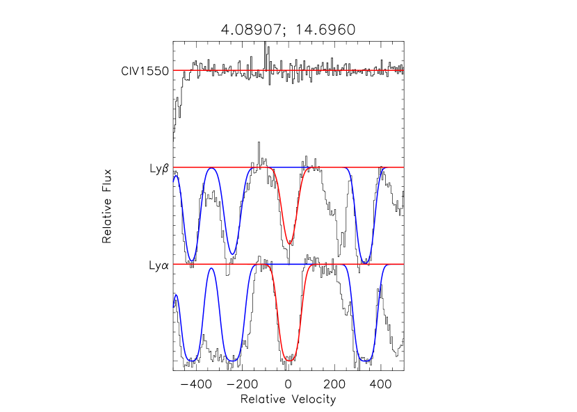
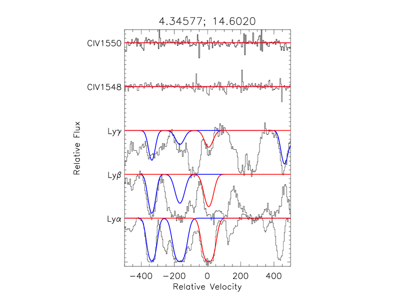
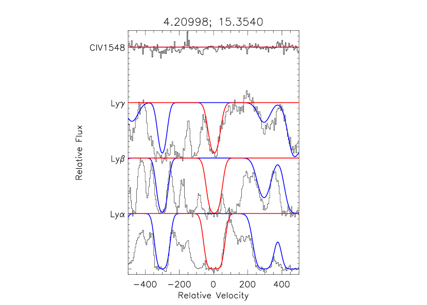
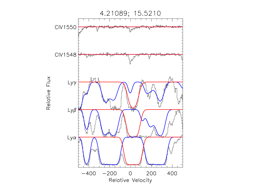
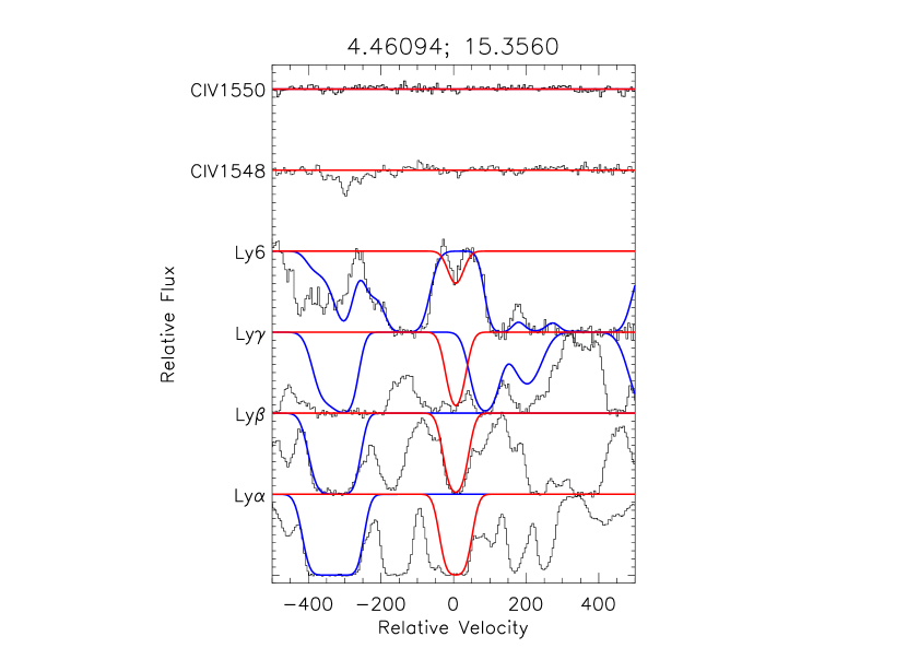
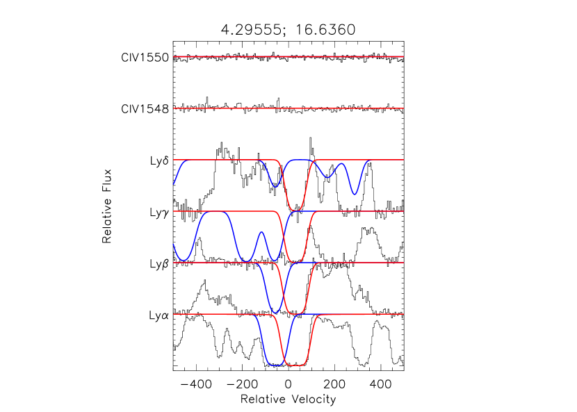
Figure 2.— Montage of absorbers and corresponding best-fit Voigt profiles, illustrating the use of partial profiles for multiple Lyman series transitions. For each plot, the column density and redshift of the line shown in red are given at top. Blue curves show blended absorption for other lines with $N_{{\rm H\;\mbox{\tiny I}}}>10^{14.5}$, which also are included in the C iv sample.

At $z=4.0-4.5$, the C iv transition falls between $\lambda=$7745Å and 8520Å. This region is rich with telluric absorption features from the atmospheric “A” and “B” bands of molecular oxygen and water. We carefully removed these features from our QSO spectra by fitting transmission functions to observations of our standard stars interspersed throughout each night.

The final 1-D spectra are shown in Figure 1. The resultant signal-to-noise ratio in the C iv region ranges from 20 to 40; in the Ly-$\alpha$ forest the ratio is somewhat lower but still suitable for measuring H i given the much greater strength of the features being measured.

3. Sample Selection

To choose our spectral search regions for C iv, we began by fitting Voigt profiles to the entire H i Ly-$\alpha$ forest using the vpfit software package. We selected $N_{{\rm H\;\mbox{\tiny I}}}\geq 10^{14.5}$ as the minimum threshold column density for an absorber to be included in the C iv candidate sample. For a standard Haardt & Madau (2001) model of the UV background field, an absorber with this column density and [C/H]=-3.0 would have $N_{{\rm C\;\mbox{\tiny IV}}}=10^{12}$cm^-2—roughly the detection limit of our data.

At $z\sim 4.3$, this H i column density corresponds to a baryonic overdensity of $\rho/\bar{\rho}=1.6$ relative to the cosmic mean (Schaye, 2001). Coincidentally, this threshold is nearly identical to the minimum $\rho/\bar{\rho}$ where individual O vi lines can be detected at $z\sim 2.5$; C iv lines can only be seen at higher overdensity at $z\sim 2.5$. Throughout the present paper we quote comparisons to both O vi and C iv samples at lower redshift.

3.1. Reliability Tests for $N_{\rm H\;\mbox{\tiny I}}$ Fits

When fitting for $N_{{\rm H\;\mbox{\tiny I}}}$ at $z>4$, much of the Lyman series is accessible provided there are no strong Lyman limit systems. We used at least three transitions of the Lyman series, and often 4 or 5 to constrain the column densities of each H i line. If no unsaturated Lyman series line or profile wing was available, a line was discarded from the sample.

Figure 2 shows several examples of H i absorbers fit in this manner, selected to span the range of column densities in our sample. Clearly there is significant blending of lines in the Ly-$\alpha$ and higher order transitions, and it is rare to have a single absorber with many unblended transitions. However roughly 60% of the sample has at least one Lyman series transition completely free of blending, and an additional 20% were significantly constrained by the unsaturated wings of blended lines in the high order transitions. Figure 3 shows a graphical summary of which transitions were used to constrain each line in the sample, over the full range in redshift.

Figure 3.— Illustration of which Lyman series lines were used in H i fits at varying redshifts. For each system, multiple transitions are used. Horizontal lines indicate components with at least partial saturation (which sometimes contain information in absorption wings). Open circles are transitions which may be blended but are not saturated in absorption and hence provide upper limits on $N_{{\rm H\;\mbox{\tiny I}}}$. Solid circles indicate distinct, apparently unblended lines which align in velocity with other Lyman series absorption.

In practice, very few systems were rejected because of saturation in all Lyman series lines. For each sightline we truncated our C iv search below the redshift where the Ly-$\gamma$ line becomes saturated from Lyman limit (or completely blended Lyman series) absorption. The high redshift boundary for each sightline is located $5000$ km s^-1blueward of the QSO’s emission redshift.

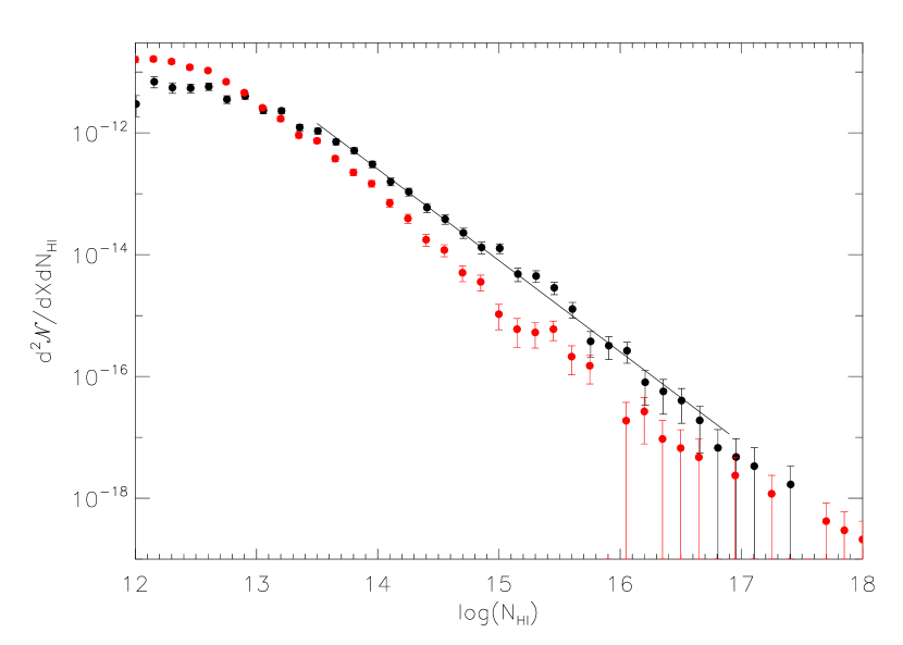
Figure 4.— The H i Column Density Distribution Function, $f_{(N_{{\rm H\;\mbox{\tiny I}}},X)}$ as measured in three sightlines at $z\sim 4.3$ (black points), and five sightlines at $z\sim 2.4$ (red points). The distributions are offset by roughly 0.5 dex, or a factor of three in normalization. Solid line shows a $N^{-1.5}$ power law, which was used as input for the Monte Carlo calculations described below.

In total, our H i sample contains 139 lines, with 13 additional candidates discarded from the sample because of saturation in the Lyman series. Just one of the discarded systems is associated with a possible C iv absorber.

When using high order Lyman transitions to constrain $N_{{\rm H\;\mbox{\tiny I}}}$, there is danger of over-estimating the column because of blended Ly-$\alpha$ absorption at lower redshift contaminating the signal. To assess this potential error, we generated Monte Carlo realizations of the Ly-$\alpha$ forest in our redshift range to test whether the fitting procedure introduces systematic errors.

The details of Ly-$\alpha$ forest line samples are not extensively characterized above $z\sim 3.5$ and it is beyond our present goals to provide a comprehensive statistical analysis of the H i forest. However, as a byproduct of our fitting procedure, we obtain a determination of the H i column density distribution at $z\sim 4.2$, shown in Figure 4. As at lower redshift, it follows a power-law form with incompleteness roll off at $N_{{\rm H\;\mbox{\tiny I}}}<10^{14}$cm^-2—well below the cutoff $N_{{\rm H\;\mbox{\tiny I}}}$ of our C iv sample. Kim et al. (2001) analyzed Ly-$\alpha$ forest spectra at $z=2.31$ and $z=3.35$, finding $f(N_{\rm H\;\mbox{\tiny I}})\propto N_{{\rm H\;\mbox{\tiny I}}}^{-1.46}$. This same shape provides an accurate fit to our observed $f(N)$ if a slightly higher overall normalization is used to account for the higher density of forest lines at $z\sim 4.2$.

For the Monte Carlo tests, we assumed this form for $f(N)$, with an overall normalization evolving as $(1+z)^{2.17}$ (Kim et al., 2001) to approximate the evolution in density of lines. Artificial spectra were generated using lines drawn from these distributions, with the full Lyman series included for each absorber. Ly-$\alpha$ lines at lower redshift were intentionally added into the Ly-$\beta$ and higher order regions at appropriate density to simulate blending and contamination. Finally, Gaussian noise was injected into each spectrum with an amplitude set by the noise arrays in our sample spectra. We do not claim the resulting spectra to be a perfect representation of the Ly-$\alpha$ forest at $z>4$, but they form a useful tool for bootstrapping estimates of our systematic errors in $N_{{\rm H\;\mbox{\tiny I}}}$ measurement from blending.

We ran VPFIT on our simulated spectra without knowledge of the input parameters, in identical fashion to the true data set. Figure 5 shows a comparison of the best-fit $N_{{\rm H\;\mbox{\tiny I}}}$ determinations with the true input values, as a function of $N_{{\rm H\;\mbox{\tiny I}}}$ and redshift. We find a scatter of $\pm 0.1$ dex between the true and fitted values, with a small systematic (median) offset of 0.04 dex in the sense that the fitted $N_{{\rm H\;\mbox{\tiny I}}}$ over-estimate the true values. Individual outliers can miss by 0.5-0.7 dex in either direction, but [65,85]% of systems are determined to better than [0.1,0.2] dex.

Figure 5.— Input vs. recovered column densities in our Monte Carlo tests of the vpfit method for selecting the H i sample. We detect an overall scatter of $\sim 0.1$ dex in determining $N_{{\rm H\;\mbox{\tiny I}}}$, with systematic offset of 0.04 dex. Ionization corrections render the effective error in [C/H] smaller than the error in $N_{{\rm H\;\mbox{\tiny I}}}$ by a factor of 3.

3.2. Comparison Sample

To study evolutionary trends, we compare the $z\sim 4.3$ C iv sample with a separate sample of absorbers at $z\sim 2.4$, taken from previously published work (Simcoe et al., 2004). In this work, O vi column densities were measured for a sample of 230 absorbers with $N_{{\rm H\;\mbox{\tiny I}}}\geq 10^{13.6}$cm^-2. A smaller sample of 83 systems were used to measure C iv absorption at $N_{{\rm H\;\mbox{\tiny I}}}\geq 10^{14}$ cm^-2.

Figure 6.— Distribution of overdensity in our H i -selected samples at $z\sim 4.3$ and $z\sim 2.4$. The C iv sample at $z\sim 4.3$ probes smaller overdensities than the $z\sim 2.4$ C iv sample, by a factor of 2. The distribution is very similar to O vi samples at lower redshift.

In Figure 6, we plot the cumulative distribution of $\rho/\bar{\rho}$ for each sample. We estimate the overdensity at each H i absorber location using the formalism of Schaye et al. (2003):

$$n_{H}=10^{-5}~{}{\rm cm^{-3}}\left({{N_{{\rm H\;\mbox{\tiny I}}}}\over{2.3\times 10^{13}{\rm~{}cm^{-2}}}}\right)^{\frac{2}{3}}T_{4}^{0.17}\Gamma_{12}^{\frac{2}{3}}\left({{f_{g}}\over{0.16}}\right)^{-\frac{1}{3}}.$$ (1)

Here, $T_{4}$ represents the temperature in units of $10^{4}$K, $\Gamma_{12}$ represents the flux of ionizing photons at the H i ionization edge, and $f_{g}$ represents the gas to total mass fraction in Ly-$\alpha$ forest systems, which is assumed to be near $\Omega_{b}/\Omega_{M}$. To obtain overdensity, we normalize this density by the mean gas density, $\Omega_{b}\rho_{c}(1+z)^{3}$. We assume $T_{4}$ to be constant and unity over the $z=2.4-4.3$ range (Schaye et al., 2000).

Figure 6 shows that the C iv sample at $z=4.3$ probes a median overdensity that is $2\times$ lower than the C iv sample at $z\sim 2.4$, despite having a limiting $N_{{\rm H\;\mbox{\tiny I}}}$ that is $3\times$ higher. The O vi sample at lower redshift probes almost an identical range in gas overdensity to the high redshift C iv sample. Therefore, comparing C iv at both redshifts removes any ambiguities in the [C/O] relative abundance but means that the high redshift sample is probing lower densities. On the other hand, comparing [O/H] at $z\sim 2.4$ and [C/H] at $z\sim 4.3$ traces the abundance evolution at fixed overdensity for an assumed value of [O/C].

Unfortunately this quantity is degenerate with one’s choice of UV background spectrum used for calculating ionization corrections (Simcoe et al., 2004; Schaye et al., 2003; Aguirre et al., 2008). In the discussions below we assume [O/C]$>0$ in the IGM, consistent with ionization by a soft spectrum composed of both galaxies and quasars (Haardt & Madau, 2001). This model is favored by pixel optical depth measurements of C iii /C iv and O vi /Si iv (Schaye et al., 2003; Aguirre et al., 2008).

We caution however that observations of the most metal-poor damped Ly-$\alpha$ systems show a recovery toward [O/C]=0 at very low metallicities(Pettini et al., 2008). Solar [O/C] ratios can be achieved with a hard background composed of quasar light with negligible galaxy contribution.

3.3. C iv Sample Definition and Measurements

For each of the H i absorbers in the sample, we examined the corresponding wavelength of the C iv doublet. Using VPFIT, we fit C iv absorption profiles to any absorbers within a velocity range of $\pm 20$km s^-1 of the H i centroid. In blended systems, we matched individual C iv components to their corresponding H i components where possible. If a single H i line contained multiple components of C iv then the total column density for these components was recorded. Finally, if no C iv is detected we used VPFIT to calculate $1\sigma$ upper limits on the C iv column density, using the error array.

Figure 7.— Cumulative distribution of C iv column densities at $z\sim 4.3$ and $z\sim 2.4$.

The final sample therefore consists of a mix of detected systems with measured column densities, and non-detections with upper limits. We used a $\geq 3\sigma$ cut as the threshold between detections and non-detections. For the non-detections, VPFIT usually finds a formal solution $N_{{\rm C\;\mbox{\tiny IV}}}\pm\sigma_{{\rm C\;\mbox{\tiny IV}}}$ with $N_{{\rm C\;\mbox{\tiny IV}}}\leq 3\sigma_{{\rm C\;\mbox{\tiny IV}}}$; the upper limit is then $N_{{\rm C\;\mbox{\tiny IV}}}+3\sigma_{{\rm C\;\mbox{\tiny IV}}}$.

The final sample of $z=4.0-4.5$ H i and C iv redshifts and column densities is presented in Table 2. The three sightlines contain 131 systems with $N_{{\rm H\;\mbox{\tiny I}}}>10^{14.5}$ Among this sample, 39 lines have C iv detections, while 92 are non-detections. The approximate limiting C iv column density is between $1-2\times 10^{12}$cm^-2.

4. Cumulative Distributions of C iv , and $N_{{\rm C\;\mbox{\tiny IV}}}/N_{{\rm H\;\mbox{\tiny I}}}$

Figure 7 shows the distribution of C iv column densities in samples drawn at the two different redshifts considered. Because the C iv samples contain a mixture of detections and upper limits, we have plotted the cumulative distribution as determined by the Kaplan-Meier estimator. The Kaplan-Meier product limit is a fundamental tool of survival statistics, which deals with censored datasets such as the one presented here (Feigelson & Nelson, 1985). Its application for measuring abundances from absorption lines is discussed in Simcoe et al. (2004).

For the Kaplan-Meier distribution to accurately represent the true distribution, two conditions must be satisfied. First, the upper limits must be statistically independent of one another, which is clearly true for the resolved, discrete absorption lines in our sample.

Second, the probability of a non-detection must not depend on the criterion used to select the sample. Since we are measuring C iv detections and upper limits for a sample selected on the basis of H i column density, this condition should hold. There may be slight discrepancies at the very high end of the H i sample because of local chemical enrichment. But because the H i column density distribution is a steep power law, the vast majority of our sample is at the low end where the censoring only depends on variation in signal-to-noise in the C iv region and is therefore quite random.

Returning to Figure 7, it is clear that the distribution of C iv evolves very little between $z\sim 2.4$ and $z\sim 4.3$. The fact that the cumulative distributions only reach $\sim 40\%$ stems from the survival analysis — recall that C iv is only detected in 39 of 131 systems, or 30%. Most of the upper limits are clustered near low $N_{{\rm C\;\mbox{\tiny IV}}}$, but some are at slightly higher values. Kaplan-Meier accounts for the difference between the fraction of detections (30%) and the value of the cumulative distribution near the limiting $N_{{\rm C\;\mbox{\tiny IV}}}$ (40%).

Figure 8.— Cumulative distribution of the C iv /H i ratio at $z\sim 4.3$ and $z\sim 2.4$. This is the fundamental observed quantity in our analysis.

The constancy of the C iv distribution with redshift has been noted by other authors, most notably Songaila (2005). Our result is consistent with these previous findings.

For studies of the IGM metallicity, our fundamental observable is $N_{{\rm C\;\mbox{\tiny IV}}}/N_{{\rm H\;\mbox{\tiny I}}}$. Because C iv evolves very little with redshift but the H i opacity increases, we expect the C iv /H i ratio to decrease toward higher redshift. The cumulative distribution of this quantity is shown in Figure 8, with the expected difference between $z\sim 2.4$ and 4.3. Note that this is the distribution of the $N_{{\rm C\;\mbox{\tiny IV}}}/N_{{\rm H\;\mbox{\tiny I}}}$ ratio for each system in the sample, not the ratio of the C iv and H i distributions. The shapes are very similar at the two epochs, with the difference coming from a systematic shift downward by roughly 0.4 dex, or a factor of 2.5.

5. Ionization Corrections

To translate the evolution in $N_{{\rm C\;\mbox{\tiny IV}}}/N_{{\rm H\;\mbox{\tiny I}}}$ into an evolution in the carbon abundance, we apply an ionization correction to each individual absorber as follows:

$$\left[{{C}\over{H}}\right]=\log\left({{{N_{{\rm C\;\mbox{\tiny IV}}}}\over{N_{{\rm H\;\mbox{\tiny I}}}}}}\right)+\log\left({{f_{{\rm H\;\mbox{\tiny I}}}}\over{f_{\rm C\;\mbox{\tiny IV}}}}\right)-\log\left({{C}\over{H}}\right)_{\sun}.$$ (2)

Here, $f_{\rm C\;\mbox{\tiny IV}}$ and $f_{\rm H\;\mbox{\tiny I}}$ represent the triply ionized fraction of carbon, and neutral fraction of hydrogen, respectively. The last term is a zero-point offset to normalize relative to the solar abundance. Throughout the paper we have assumed the meteoric Solar abundances of Grevesse & Sauval (1998), where $A_{\rm carbon}=8.52$ on a scale with $A_{\rm Hydrogen}=12$. Several revisions have been proposed to the Grevesse solar abundances (Allende Prieto et al., 2002, 2001; Holweger, 2001); we have kept them for consistency with prior work by many authors on IGM abundances.

Ionization fractions for carbon and hydrogen were determined using the CLOUDY (Ferland et al., 1998) software package. We assumed the IGM is optically thin (consistent with the low H i column densities in the sample), and in photoionization equilibrium.

5.1. Comments on choice of the UV background spectrum

Figure 9.— Mean spectrum of the UV background radiation field, at $z\sim 4.3$ and $z\sim 2.4$. We show the calculations of both Haardt & Madau (2001, including a galaxy contribution) and Faucher-Giguère et al. (2009) for comparison. The spectra are very similar at high redshift; at lower redshift the Faucher-Giguère et al. (2009) version is harder, leading to higher overall abundances and a correspondingly larger evolution in the observed [C/H] ratio.

The largest uncertainty in our ionization correction arises from the choice of a particular prescription for the ionizing background spectrum.

Several groups have recently provided improved constraints on the overall intensity of the background field at 1 Rydberg - denoted as $J_{912}$. This can be derived from the opacity of the Ly-$\alpha$ forest, which relates in turn to the H i photoionization rate $\Gamma_{12}$. In a sample of 63 high resolution spectra spanning $2.0<z<5.5$, Becker et al. (2007) find $\Gamma_{12}=[0.8,0.5]$ at $z=[2.4,4.3]$, where by convention $\Gamma_{12}$ is normalized to units of $10^{-12}{\rm s}^{-1}$. Faucher-Giguère et al. (2008a) find $\Gamma_{12}=[0.6,0.4]$ over the same range using slightly different analysis techniques on a set of 86 high resolution spectra. Earlier analyses by Bolton et al. (2005) and Scott et al. (2000) derived slightly higher estimates closer to $\Gamma_{12}=1$. However, all of these studies find that the evolution of the H i photoionization rate is quite weak over the redshift range studied here, perhaps $10-30\%$ smaller at $z=4.3$ but not much more. Throughout the rest of the paper, we use the values from Becker et al. (2007). For a power law ionizing spectrum $\propto\nu^{-1.8}$, this corresponds to a flux at the H i ionization edge of $\log(J_{912})=[-21.5,-21.7]$ at $z=[2.4,4.3]$.

Even if the normalization of the background spectrum at 1 Rydberg does not evolve, it is generally agreed that the shape of the spectrum will change. The quasar luminosity function falls off between $z=4$ and $z=2$ (Hopkins et al., 2007). While ionizing photons at $z=2.4$ come from both quasars and galaxies, the background at $z=4.3$ contains a higher fractional contribution from galaxies (Faucher-Giguère et al., 2008a). This should lead to a softer UV background at earlier epochs, with fewer photons at the higher energies which regulate the ionization balance of heavy elements like carbon and oxygen.

Figure 10.— Neutral fraction of hydrogen as calculated by CLOUDY, compared with the analytic approximation of Equation 3. This relation is redshift-independent, except for the implicit dependence on the IGM temperature and $\Gamma_{12}$. It has a logarithmic slope of $\frac{2}{3}$ dex change in $f_{\rm H\;\mbox{\tiny I}}$ per unit dex in $N_{{\rm H\;\mbox{\tiny I}}}$.

We have tested two main prescriptions of the UV background with our data: the commonly used version from Haardt & Madau (2001), and an independent new determination from Faucher-Giguère et al. (2009). In Figure 9 we show these spectra, with the energies of relevant transitions for the C iv ionization balance labeled. The Haardt  & Madau spectrum includes contributions from both QSOs and galaxies; the QSO portion is determined from the Croom et al. (2004) luminosity function, while the galaxies are added through population synthesis modeling, assuming a 10% escape fraction of photons beyond the Lyman limit. The Haardt& Madau spectra have been normalized to match the observational constraints on $\Gamma_{12}$ described above. Faucher-Giguère et al. (2009) take the QSO luminosity function from Hopkins et al. (2007) which falls more steeply toward higher redshift, and add a galaxy contribution to keep the evolution of $\Gamma_{12}$ constant.

When the Haardt & Madau spectrum is renormalized in CLOUDY to match observations of $\Gamma_{12}$ at 13.6 eV, its soft X-ray background is also artificially boosted by a factor of $\sim 10$ at energies above 10 Rydbergs. This has consequences for the C iv ionization balance because it affects the C v to C vi transition.

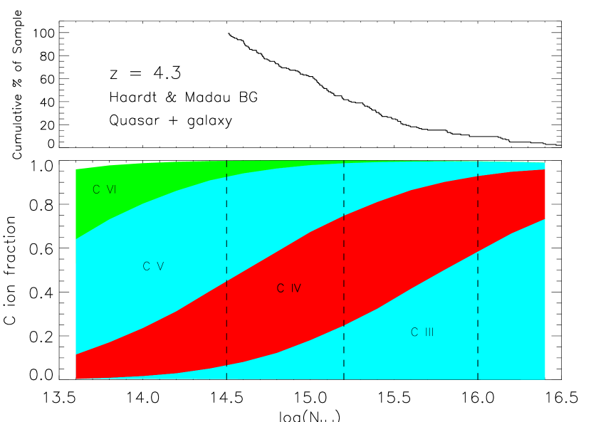
Figure 11.— CLOUDY carbon ionization balance at redshift $4.3$ for the Haardt & Madau (2001) model of the UV background (top) and Faucher-Giguère et al. (2009, bottom) models. The histogram at top indicates the cumulative distribution of lines in our sample, with the minimum, median, and 90th percentile shown by vertical lines. At this redshift, the C iv fraction peaks in the IGM, at $f_{\rm C\;\mbox{\tiny IV}}\sim 0.5$.

In their calculations, Haardt & Madau treat the UV and X-ray backgrounds independently, trying to match each with observed luminosity functions by balancing the relative importance of Type I and II QSOs. In its raw form, the Haardt & Madau X-ray background is slightly lower at z=4.3 than at 2.4 (as would be expected), but after renormalization to matched the observed $\Gamma_{12}$ at 1 Ry, the situation reverses, such that the X-ray background is higher at $z=4.3$ than it is at $z=2.4$. Since the X-rays originate in AGN which are proportionately fewer at high redshift, this situation is probably unphysical. So, we applied a downward correction of 0.8 dex to the $z=4.3$ HM spectrum above 10 Ryd to soften it by a comparable amount as the UV background and bring it back into agreement with the original X-ray intensity. Coincidentally, this downward correction brings the HM spectrum into fairly close agreement with the Faucher-Giguère et al. (2009) spectrum, which by construction does not suffer from this effect of renormalization.

While the HM and Faucher-Giguère et al. (2009) spectra do not agree in every detail, their general shapes match fairly well, particularly at $z=4.3$. At lower redshift the difference is larger owing to assumptions on the AGN contribution as well as the treatment of He ii reionization. However, in both models the main change from $z=2.4$ to $z=4.3$ is a factor of 10-20 decrease in the hard UV background. It should be noted that neither model captures the He ii “sawtooth” effect described in Madau & Haardt (2009); this is discussed in Section 6.3.5.

5.2. H i ionization fractions

Since the Ly-$\alpha$ forest is optically thin and in photoionization equilibrium, a calculation of $f_{{\rm H\;\mbox{\tiny I}}}$ is relatively straightforward and may be made even without detailed knowledge of the spectral shape. In equilibrium, the ionization and recombination rates may be balanced as:

$$f_{{\rm H\;\mbox{\tiny I}}}n_{H}\Gamma\approx n_{H}^{2}R$$ (3)

where the recombination rate $R\approx 4\times 10^{-13}T_{4}^{-0.76}$ cm³s^-1, $n_{H}$ is given in Equation 1, and we assume the gas is mostly ionized. Equations 1 and 3 may be combined to derive the hydrogen ionization fraction as a function of (observed) H i column density, plotted in Figure 10 alongside its numerical CLOUDY determination. This relation is independent of redshift, except implicitly through the (weak) evolution of the ionization rate $\Gamma$, and the temperature $T_{4}$.

5.3. C iv ionization fractions

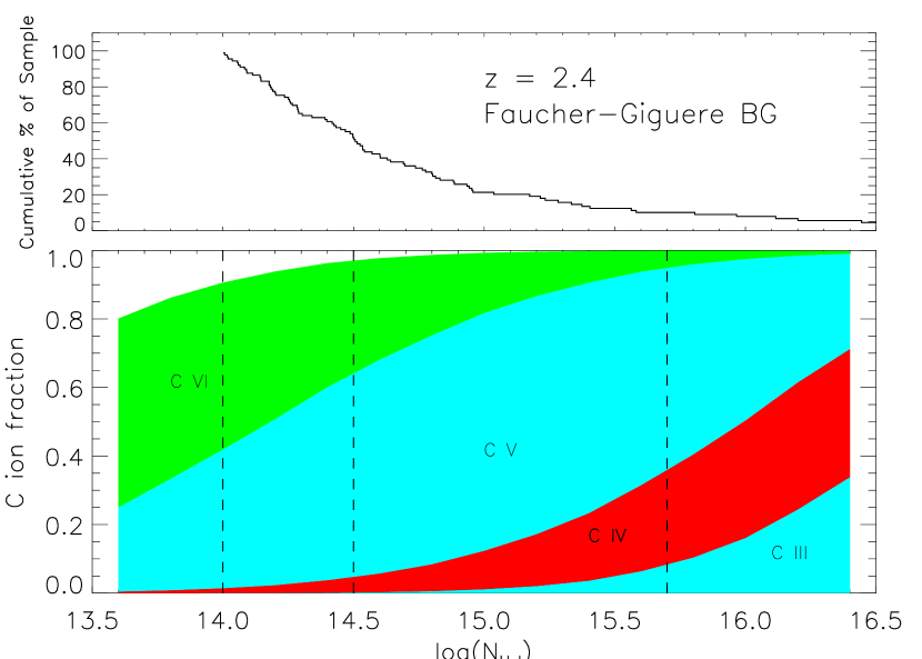
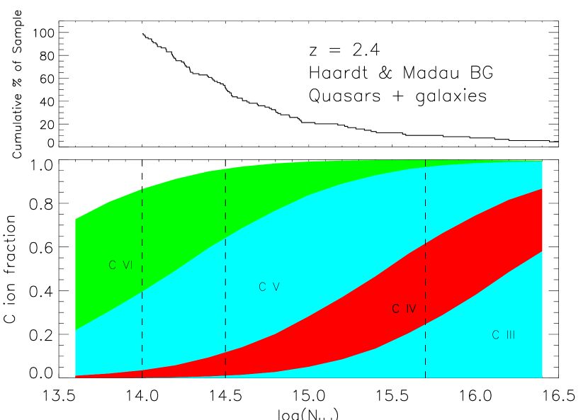
Figure 12.— CLOUDY carbon ionization balance at $z\sim 2.4$, again for both models of the UV background. The mean H i column density is lower, as is the ionization fraction in C iv. The lower ionization fraction may be directly mapped to the inferred change in abundance.

The ionization balance of C iv is a far more difficult calculation, because it is governed by photons at frequencies where the UV background spectrum is less well constrained observationally. Figure 11 shows the CLOUDY-derived ionization balance for carbon as a function of H i column density, at $z=4.3$ (the balance at $z=2.4$ is shown in Figure 12). To calculate the ionization fractions, we first estimated the total hydrogen density associated with each H i column density as calculated from Equation 1. This value of $n_{H}$ was input into CLOUDY along with the prescriptions shown in Figure 9 for the shape and amplitude of the background spectrum. Together, the determinations of the density and ionizing background flux determine the ionization parameter $U$ for the cloud which allows CLOUDY to calculate the abundance fraction of each carbon ionization state.

The top panel of each figure shows the cumulative distribution of H i column densities for the C iv samples, as a visual aid to indicate what ionization corrections are appropriate for which fractions of the sample. Vertical lines on the bottom panels indicate the sample minimum $N_{{\rm H\;\mbox{\tiny I}}}$, and also its median value and 90th percentile. Plots are shown both for the Haardt & Madau and Faucher-Giguere forms of the background spectrum.

These plots show that the C iv ionization state predominates at $z\sim 4.3$, at a value of $f_{\rm C\;\mbox{\tiny IV}}=0.50-0.65$ for the median H i system in the sample. This range reflects the difference between the Haardt & Madau (2001) and Faucher-Giguère et al. (2009) backgrounds, respectively. Roughly equal amounts of carbon are in higher and lower ionization states.

Conversely, the median system at $z\sim 2.4$ contains only 4-10% C iv , with the vast majority of carbon inhabiting higher ionization states. So, the typical ionization correction at $z=4.3$ is an upwards factor of 1.5-2.0 (0.2-0.3 dex), compared to a correction factor of $10-25$ (1.0-1.4 dex) at lower redshift.

6. Abundance Results

6.1. Evolution from $z=4.3$ to $z=2.4$: Qualitative Results

Before presenting the full carbon abundance distribution results, it is instructive to examine the evolution of the median system using qualitative arguments. From Figure 8, the median H i absorber decreases in its C iv:H i ratio by 0.4 dex between $z=4.3$ and $z=2.4$.

Suppose now that there were no evolution in the [C/H] ratio. To achieve this, our measured 0.4 dex decrease in C iv /H i would need to be offset by a corresponding 0.4 dex increase in $\log\left({f_{\rm H\;\mbox{\tiny I}}}/{f_{\rm C\;\mbox{\tiny IV}}}\right)$, according to Equation 2.

We have seen already that $f_{\rm H\;\mbox{\tiny I}}$ depends on $N_{{\rm H\;\mbox{\tiny I}}}$ but only very weakly on redshift. For a median $\log(N_{{\rm H\;\mbox{\tiny I}}})=14.5$ at $z=2.4$ and $15.2$ at $z=4.3$, the H i ionization fractions can be read from Figure 10, yielding $\log(f_{{\rm H\;\mbox{\tiny I}},4.3})-\log(f_{{\rm H\;\mbox{\tiny I}},2.4})\approx 0.5$.

Thus for fixed $f_{\rm C\;\mbox{\tiny IV}}$, the first term in Equation 2 is 0.4 dex lower at $z\sim 4.3$, while the second is 0.5 dex higher. The first term is observationally determined, and the second is fairly model-independent, and they approximately cancel each other out. The degree of evolution in [C/H] therefore corresponds almost exactly to the change in $f_{\rm C\;\mbox{\tiny IV}}$ with redshift.

Even if we take the most conservative possible hypothesis - that the UV background spectrum at $z=4.3$ is identical to the spectrum at $z=2.4$ - then $U$ will decrease because of the increase in gas density at higher redshift. But observational studies of the QSO and galaxy luminosity functions at these redshifts indicate that the background spectrum should soften as it is increasingly dominated by galaxies toward higher redshift (Faucher-Giguère et al., 2008a). These factors cause an increase in $f_{\rm C\;\mbox{\tiny IV}}$ which leads to a decrease in implied [C/H]. Thus the observed distribution of $N_{\rm C\;\mbox{\tiny IV}}/N_{\rm H\;\mbox{\tiny I}}$, coupled with minimal assumptions about ionization, suggest that [C/H] is lower at $z=4.3$ than it is at $z=2.4$.

To estimate by how much, consider the CLOUDY calculations from both the Haardt & Madau (2001) and Faucher-Giguère et al. (2009) spectra. These illustrate that the C iv ionization fraction for the median system increases by 0.7 dex toward higher redshift. Taken together, these qualitative arguments suggest that [C/H] in the median system is lower at $z\sim 4.3$ by 0.5-0.6 dex (a factor of $\sim 3$) than it is at $z=2.4$.

They also suggest that the scatter in the C iv to H i ratio may be an interesting diagnostic of fluctuations in the hard UV background. The scatter in this ratio reflects the convolved scatter in the intrinsic [C/H] ratio, measurement errors, and variance in the ionization correction. Even if one makes no assumptions about the relative weighting of these three factors, one may set upper bounds on the scatter in the hard background under the conservative assumption of zero measurement error and abundance scatter.

6.2. The Cumulative [C/H] Distribution at $z\sim 4.3$

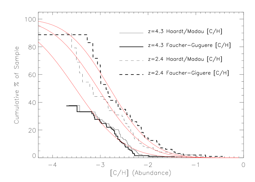
Figure 13.— Kaplan-Meier cumulative probability function for carbon abundance in the IGM at $z\sim 4.3$ and $z\sim 2.4$. Note that the low redshift curves sample the IGM at a median overdensity roughly $2\times$ larger than the high redshift sample. Solid curves indicate lognormal probability distributions. At $z\sim 4.3$, the curve represents a median abundance of [C/H]=-3.65, and $\sigma=0.8$. At lower redshift the median rises to [C/H]=-3.1 for the Haardt & Madau (2001) background, or [C/H]=-2.8 for Faucher-Giguère et al. (2009), with similar scatter. The difference of 0.5-0.7 dex represents a $3-5\times$ increase in the median abundance for the low redshift sample.

Figure 13 shows the Kaplan-Meier distribution of [C/H] at $z=4.3$ and $z=2.4$, derived by applying ionization corrections individually to each C iv system (or its upper limit). The distributions are shown for both the Haardt & Madau (2001) and Faucher-Giguère et al. (2009) forms of the UV background radiation field. Recall that we show the [C/H] distributions for each redshift to eliminate ambiguity in [O/C], but the $z=4.3$ sample probes gas with a median overdensity of $\rho/\bar{\rho}\approx 3$, whereas the C iv sample at $z=2.4$ only reaches a median $\rho/\bar{\rho}\approx 6$ (the sample minima are $\rho/\bar{\rho}\approx 1.6$ and $\rho/\bar{\rho}\approx 3$).

At $z=4.3$, our sample reaches nearly to the median [C/H] ($50\%$ on the plot), which lies near [C/H]$=-3.55$, or $\sim 1/3500$ the Solar abundance. Roughly half of the lines in our sample have $3\sigma$ upper limits restricting them below this value, so the shape of the distribution below the median is not known. Above the median, the distribution appears to be very crudely lognormal, with the upper quartile falling above [C/H]$=-3.1$. The distributions are very similar for the two choices of UV background radiation spectrum at $z=4.3$. The smooth solid curve shows the cumulative distribution for a lognormal probability distribution. Our best fit lognormal model shows a median abundance of [C/H]=-3.55, and lognormal deviation of $\sigma=0.8$ dex.

At $z=2.4$, we find a median abundance of [C/H]$=-3.1$ with $\sigma=0.8$ dex for the Haardt & Madau (2001) form of the background spectrum, consistent with prior results of Simcoe et al. (2004) and close to, though slightly higher than those of Schaye et al. (2003). The Faucher-Giguère et al. (2009) form of the background spectrum results in a slightly higher carbon abundance but similar scatter, at median [C/H]=$-2.8$ and $\sigma=0.7$ dex. The higher median results from the increased flux in the Faucher-Giguère et al. (2009) spectrum near 5 Rydbergs, at the C iv to C v ionization edge. This flux enhancement favors higher ionization and hence larger ionization corrections.

Comparing the two distributions, we see that the sample median carbon abundance has increased by $\sim 0.45-0.65$ dex (depending on the background model) during the epoch between $z=4.3$ and $z=2.4$, although the density probed at $z\sim 2.4$ is a factor of 2 larger. It is interesting to compare this result to that of Schaye et al. (2003), who find $d/dz([{\rm C/H}])=+0.08^{+0.09}_{-0.10}$ and $d/d(\log(\rho))({\rm[C/H]})=0.65^{+0.10}_{-0.14}$. Not accounting for density, our measurement implies a derivative of roughly $-0.26$ dex per unit redshift, a factor of $3.3$ higher than reported by Schaye et al. Moreover the evolutionary trend has the opposite sign as Schaye’s; our new result evolves in the expected direction (i.e. increasing abundance with time), although the prior result was basically consistent with zero evolution.

Since Schaye et al. reported weak correlation with redshift but strong correlation with density, it is worth considering whether our measured evolution is simply an artifact of the different densities probed at the different redshifts. According to the regression analysis of Schaye et al., a $2\times$ change in density alone could account for $\approx 0.3$ dex difference in [C/H] between the samples, but their reported evolution of +0.08 dex per unit redshift for $\Delta z=1.9$ would counteract the density effect by 0.15 dex, yielding a total change in [C/H] of 0.15 dex to our 0.5. Schaye et al interpret the small statistical significance of their evolution coefficient and its non-intuitive sign as a non-detection. We have detected a larger difference in [C/H] between our high and low redshift samples, in the expected direction, even accounting for the difference in density.

To decouple the effects of density and true evolution, we ran our analysis for a subset of our high redshift sample restricted to $\log(N_{{\rm H\;\mbox{\tiny I}}})\geq 10^{14.7}$, thus ensuring that [C/H] is measured at fixed overdensity between the two redshifts. The resulting Kaplan-Meier distribution is shifted to higher [C/H] by 0.2 dex for this factor of 2 increase in $\rho/\bar{\rho}$, suggesting that the abundance is indeed lower in regions of smaller overdensity, but by a smaller degree than measured by Schaye et al. If we budget 0.2 dex of the total 0.5 change seen in Figure 13 to the change in gas density, the remaining 0.3 dex represents the temporal evolution signal.

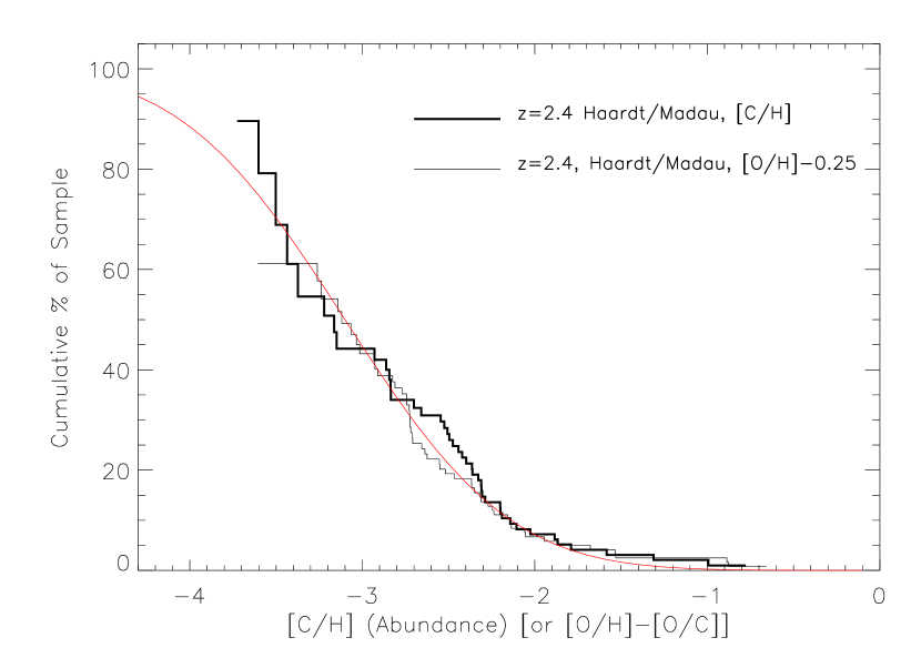
Figure 14.— Kaplan-Meier Distribution function for Carbon and Oxygen in the $z\sim 2.4$ IGM, used for calibrating the [O/C] ratio, which is best fit with [O/C]=0.25. A positive [O/C] has been found by many authors, though the value used here is slightly smaller than other estimates in the literature (see text).

As described earlier, we may also compare our measurements of [C/H] at $z\sim 4.3$ to pre-existing measurements of [O/H] at $z\sim 2.4$, which cover an identical range of overdensity bust must be corrected for any non-Solar value of [O/C]. We estimate the value of [O/C] by comparing the [O/H] and [C/H] distributions at $z\sim 2.4$, and applying this same value at $z=4.3$ (i.e. assuming no evolution in relative solar abundances). Figure 14 shows the result of this calculation. The [C/H] distribution is shown in the thick solid line, while the [O/H] distribution is the thin line; here the [O/H] curve has been shifted downward by 0.25 dex, simulating the predicted [C/H] for a best-fit [O/C]=0.25. Other studies (Simcoe et al., 2004; Schaye et al., 2003; Aguirre et al., 2008) have generally found positive [O/C] distributions for soft photoionizing spectra, with values near [O/C]$\sim 0.5$. Our slightly smaller value likely results from a slightly higher normalization of the background spectrum to match recent observations (Becker et al., 2007; Bolton et al., 2005). The best-fit [O/C] for the (Faucher-Giguère et al., 2009) UV background is near [O/C]=0, which is to be expected considering that this spectrum is much harder than the (Haardt & Madau, 2001) background at $z=2.4$.

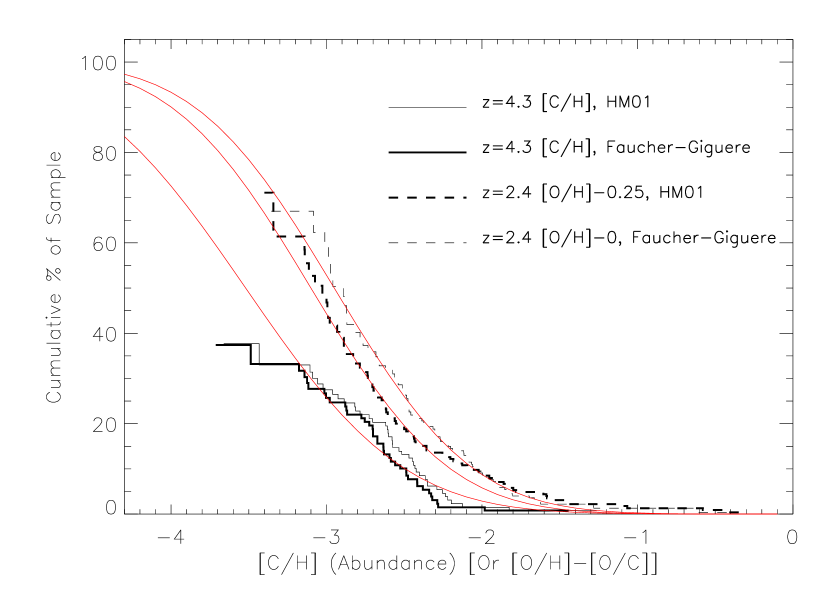
Figure 15.— Kaplan-Meier Distribution function for [C/H] at $z\sim 4.3$ and [O/H]-0.25 at $z\sim 2.4$. Subject to estimates of [O/C], this distribution is our best representation of the change in [C/H] at fixed overdensity. The curve at $z\sim 4.3$ is the same as in Figure 13; the lognormal fits shown here for $z\sim 2.4$ have a median [C/H]=-3.1, -2.9 for the two models of the UV background.

Figure 15 shows the distributions of [C/H] at $z=4.3$, [O/H]$-0.25$ at $z=2.4$ for the Haardt & Madau (2001) UV background, and [O/H] for the Faucher-Giguère et al. (2009) model (which has best-fit [O/C]=0). Lognormal curves are show for each model. The two $z=2.4$ models have median abundances of $-2.9$ and $-3.1$, with similar scatter. Evidently there is a 0.5 dex evolution in the median [C/H] at fixed overdensity for [O/C]=0.25; adopting [O/C]=0.5 would reduce the absolute change by 0.25 dex.

Figure 16 shows this evolution as evidenced in the individual sample measurements at each redshift. The large circles show our median estimates at each redshift, while the central point is taken from Schaye et al. (2003)

Taken all together, these calculations indicate that the intergalactic carbon abundance increased by 0.3-0.5 dex between $z\sim 4.3$ and $z\sim 2.4$, with little change in the lognormal abundance scatter. The range quoted reflects uncertainty in various choices for the UV background, the relation between density and metallicity, and the value of [O/C] used.

A change of 0.3-0.5 dex represents a factor of $\sim 2-3$ increase in the median intergalactic carbon abundance at fixed overdensity. It suggests that roughly half of the carbon seen in the IGM at $z\sim 2.4$ was deposited in the 1.3 Gyr interval between $z\sim 4.3$ and $z\sim 2.4$.

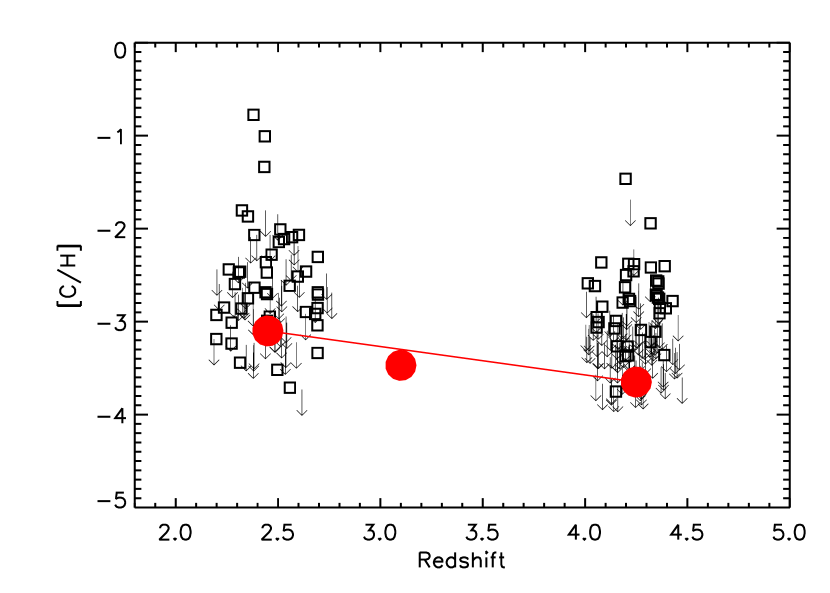
Figure 16.— Illustration of the individual measurements for each line in the full sample. Large red dots indicate the median abundance at each redshift, calculated using the Kaplan-Meier product limit estimator. The median points lie below the center of the scatter because of the inclusion of numerous upper limits. The solid point at $z=3.1$ represents the measurement of Schaye et al. (2003).

6.3. Uncertainties

6.3.1 Ionizing Background Fluctuations

The results presented above all assume a spatially uniform shape and intensity of the ionizing background, following the convention of all similar previous studies. Although we find similar results for two representations of the mean background (Haardt & Madau, and Faucher-Giguere), we did not explore the uncertainty or scatter that would be introduced by place-to-place variations in the radiation field.

This subject has largely been ignored in the previous literature on IGM abundances, but recent work on the reionization of H i and He ii contains arguments that are relevant to observations of heavy element lines.

Following the development of Fardal et al. (1998) and Meiksin & White (2003), the variance in the background intensity at a given energy is a function of the source density of photon emitters at that energy, the mean free path of photons with that wavelength through the IGM, and the variance in source spectrum from object to object. When ionizing sources are rare, differ in SED from object to object, and photons have a small mean free path, the radiation seen by a random absorber tends to be dominated by a single source and will vary significantly from place to place.

The production of H i ionizing photons at $z=4.3$ occurs mostly in galaxies which are relatively numerous, and the mean free path for these photons is large because H i is already reionized. So, many sources will be contained within an H i photo-attenuation volume and the background should be comparatively uniform at 1 Ryd (except in the immediate vicinity of QSOs).

Overall variations in [C/H] are therefore more sensitive to the C iv ionization balance, whose atomic transitions are resonant with photons between $3-30$ Rydbergs. These photons originate in less numerous AGN, which could lead to an increased variation in spatial intensity. Since our high redshift sample is measured at the probable leading edge of He ii reionization (Reimers et al., 1997; Jakobsen et al., 1994; Heap et al., 2000; Davidsen et al., 1996; Kriss et al., 2001; Fechner et al., 2006; Shull et al., 2010; Songaila, 1998), the IGM opacity from photoelectric absorption must be considered above the He ii ionization potential (4 Ryd).

For photons of energy $E$, the mean free path is given as (Furlanetto, 2009)

$$\lambda=0.41\left({1+z}\over{5.3}\right)^{-2}\left({E}\over{4{\rm~{}Ryd}}\right)^{3}\bar{x}_{{\rm He\;\mbox{\tiny II}}}^{-1}~{}{\rm Mpc}$$ (4)

At $z=4.3$, $x_{{\rm He\;\mbox{\tiny II}}}\approx 1$ since He ii reionization is only in its earliest phases. For C iv $\rightarrow$C v ionizing photons with 4.74 Ryd, this implies $\lambda<1$ Mpc because of He ii attenuation, while for C v $\rightarrow$C vi  (24.2 Ryd) the path is $90$ Mpc. Thus the most important effect we must consider is stochastic fluctuation in the 4.74 Ryd background governing the C iv to C v transition.

At $z=4.3$, simulations indicate that 10-20% of the universe resides in ionized “bubbles” of He iii (McQuinn et al., 2009). He ii Ly-$\alpha$ observations focus only on the interiors of these bubbles, where the ionized fraction is high and He ii absorption troughs are not totally saturated. The lower oscillator strength of C iv renders it observable in both He iii ionized bubbles, and the He ii -neutral walls in between. In the bubble walls, He ii absorption strongly attenuates the UV background near 4 Ryd, affecting the ionization balance of carbon. Inside of bubbles, stochastic variations in the proximity of hard photon sources and attenuation by He ii Lyman-limit systems generates intensity variations both above and below the mean spectrum. In the following two sections we consider each of these environments in separate detail.

6.3.2 UV background fluctuations in the interior of He iii bubbles

To study ionization variations of carbon inside He iii bubbles, we follow the arguments of Furlanetto (2009), who develops a simple Monte Carlo framework suited to the problem. The method was originally intended for studying variations in the 4 Ryd background in He iii bubbles at $z\sim 3$; a minor set of modifications renders it useful for studying the C iv $\rightarrow$C iv transition at at $E=4.74$ Ryd and $z=4.3$. Essentially all opacities in the model are scaled down to reflect the smaller cross section of He ii at higher energy, and fluxes from the ionizing sources is also scaled down to reflect their SED.

We defer a full description of the method to Furlanetto’s paper. Very briefly, all quasars are assumed to live inside of He iii-ionized bubbles. The space outside of bubbles is opaque to He ii-edge photons; inside of bubbles there is still attenuation from the He ii analog of Lyman limit systems, but between these systems the mean free path is large.

Because QSOs are rare, the typical bubble contains only one to a few sources, so a Monte Carlo approach is used. Ionizing sources are drawn at random from the luminosity function of Hopkins et al. (2007), and placed uniformly within each bubble volume (no sources are located outside of bubbles). Then, the spatial variation of the background $J$ is calculated by compiling trial statistics with varying QSO luminosities, spatial locations in the bubble, Lyman limit attenuation, and UV spectral indices from the sources.

The Monte Carlo calculation outputs a distribution of $j=J/\left<{J}\right>$, where $\left<{J}\right>$ represents the mean value of the background in a fully He ii-ionized IGM. The $J$ distribution at the C iv $\rightarrow$C v ionization edge can be used to examine variations in our C iv ionization corrections.

The spread of $j$ depends strongly on the radii of the He iii bubbles, denoted as $R$, since variations diminish once bubbles become large enough for absorbers to “see” multiple QSOs. McQuinn et al. (2009) and Bolton et al. (2009) have shown in simulations that the distribution of $R$ does not evolve strongly with redshift and is governed primarily by QSO duty cycle. Typical values range from $20-40$ comoving Mpc, with the spread at any redshift larger than the difference between $z=4$ and $z=2$. The spread in $j$ also depends on the photoattenuation length $r_{0}$, which parameterizes the distance that C iv ionizing photons travel from their point of origin before reaching a He ii lyman limit system. Furlanetto (2009) calculates $r_{0}$ for He ii ionizing photons at $z=2,3,4$ and demonstrates that its luminosity-weighted mean evolves very little. C iv ionizing photons have slightly higher energies; their attenuation is still dominated by He ii absorption, but the relevant $r_{0}$ increases very slightly because of the smaller He ii cross section at 4.74 Ryd.

Figure 17.— Distribution function of flux at the C iv $\rightarrow$C v ionization edge, in He iii-ionized bubbles at $z\sim 4.3$. The flux is normalized in units of the mean, $\left<{J}\right>$. Scatter above the mean is dominated by proximity to individual QSOs, which enhances the background over a wide range of frequencies above 1 Ryd. Scatter on the low side arises from stochastic variations in the density of nearby QSOs and shielding from He ii patches.

Figure 17 shows the distribution of $J$ at $4.74$ Ryd in logarithmic (top panel) and linear (bottom panel) forms, for bubbles ranging from $R=15$ to 50 comoving Mpc. In all cases we have assumed $r_{0}=35$ Mpc, as in Furlanetto (2009). As expected, the shape is very similar to what was derived for He ii by Furlanetto (2009), except the distributions are slightly narrower because of the increased transparency of He ii at 4.74 Ryd. Above the mean background flux, the curves converge for all bubble sizes. Furlanetto (2009) observed this same effect for He ii; it represents environments where the background is dominated by a single source. In this case the variance is driven by the shape of the QSO luminosity function and the random distribution of QSO-absorber spacings.

According to Figure 17, variations on the high-side are limited to a factor of $\sim 10\times$ enhancement in the background. Because this enhancement is driven by proximity to a single QSO, it should lead to an increase in the UV background across a wide range in frequency. When examining the C iv ionization balance in these neighborhoods, we generate an “enhanced” toy model of the background spectrum which boosts the flux for all energies above 1 Ryd by a constant factor of $5-10$. Below 1 Ryd the background remains the same, since it should still be dominated by integrated starlight from more numerous galaxies.

Below the mean $J$, the distribution in Figure 17 is more extended and varies with bubble size. The increased variance for small bubble sizes results primarily from shot noise in the number of quasars: by $R=15$ Mpc most bubbles have either no source or one source, and sources outside the bubble are shielded from view. This effect is strongest at the He ii ionization edge, and still significant at 4.74 Ryd. But the bubble walls are optically thin to photons with $E<4$ Ryd and also for higher energy photons including the $24.2$ Ryd C v $\rightarrow$C vi edge. Thus it is appropriate simply to use the mean UV background spectrum for H i , as well as all carbon transitions except C iv $\rightarrow$C v (and possibly C iii $\rightarrow$C iv , see Section 6.3.5).

To model effects at 4.74 Ryd, we attenuate the Haardt & Madau (2001) spectrum by an absorbing column with $\tau=\tau_{0}(E/4{\rm Ryd})^{-3}$. This produces the desired suppression at $4.74$ Ryd while preserving the cosmic averaged spectrum in optically-thin regions. The normalization $\tau_{0}$ is adjusted to produce a factor of 10-100 decrease in the background at 4.74 Ryd, consistent with the distribution in Figure 17.

Figure 18.— Model UV background spectra used to evaluate the effects of variations on our inferred [C/H] estimates. The thick solid line represents the mean Haardt & Madau (2001) background. Curves below this mimic the suppression of 4.74 Ryd photons by He ii Lyman limit systems (inside of bubbles) or the neutral walls between bubbles. Curves above the mean represent the proximity zones of QSOs.

6.3.3 UV background fluctuations in the He ii -neutral inter-bubble medium

In simulations of He ii reionization, He iii bubbles only permeate 10-20% of the IGM by volume, so we must consider the shape of the spectrum in the He ii walls between bubbles. This scenario is discussed in Faucher-Giguère et al. (2009); essentially flux at the He ii edge is completely suppressed because in He ii-neutral regions the optical depth can easily exceed $\tau\sim 100$. Once again, the background at lower energies is spatially uniform, being optically thin after H i reionization (and, for low energies, dominated by galaxies). Likewise at higher energies the He ii cross section declines and the hard flux recovers to a uniform background.

We therefore model the background spectrum in He ii walls the same as in the “suppressed flux” regions of ionized bubbles: a Haardt & Madau (2001) standard mean background having He ii absorption blueward of the edge with $\tau=\tau_{0}(E/4{\rm Ryd})^{-3}$. However in the neutral walls the normalization of optical depth is much higher. Whereas attenuation from Lyman limit systems in bubbles reduces the flux by a factor of 10-100, the completely neutral bubble walls with $\tau\sim 100$ experience attenuation by 44 orders of magnitude.

6.3.4 The effect of spatial fluctuations on [C/H] estimates

Figure 19.— CLOUDY calculations showing correction factors to the ionization term in Equation 2. In regions where the 4.74 Ryd background is suppressed, little or no change is apparent. In regions of enhanced flux and high density, we may overestimate the abundance by up to $\sim 1$ dex.

Figure 18 shows the range of ionizing background models we considered when investigating spatial fluctuations. The thick solid line represents the mean Haardt & Madau (2001) quasar+galaxy spectrum at $z=4.3$. Four models with He ii attenuation of $\tau_{0}=1,3,10,100$ fall below the mean. Smaller values of $\tau_{0}$ represent conditions on the lower half of the $J$ distribution inside of He iii bubbles, the larger values are characteristic of the He ii bubble walls. Above the mean curve are two models with enhanced hard UV flux (i.e. proximate to QSOs), shown in dot-dashed lines.

We ran each of these spectra through our CLOUDY model grid to examine the change to the ionization fraction as a function of column density. Figure 19 shows the result of this exercise, where we plot the change in ionization correction for each different choice of background spectrum. A value of zero indicates no change in [C/H] for a given line; a positive value implies a lower metallicity for a given set of C iv and H i measurements.

The solid lines near zero represent the four “attenuated” models with varying optical depth at 4 Ryd, increasing upwards. For these models the H i ionization fraction does not change at all because the universe is already optically thin to 912 Å photons at $z\sim 4.3$ and the background is dominated by flux from numerous galaxies. The C iv ionization fraction does not change either, which results in a very small total correction of $\lesssim 0.2$ dex to [C/H] across our range of $N_{{\rm H\;\mbox{\tiny I}}}$.

The small change in $f_{{\rm C\;\mbox{\tiny IV}}}$ is surprising at first glance given that the flux at the C iv $\rightarrow$C v ionization edge changes by many orders of magnitude. The reason this effect is so small is that even for the mean spectrum, over 50% of the carbon is already in the C iv state. So, a reduction in the C iv $\rightarrow$C v rate—which would increase $f_{\rm C\;\mbox{\tiny IV}}$—cannot change the C iv fraction by more than a factor of $\sim 2$.

A much larger correction is obtained when considering upward fluctuations in the UV background from proximity to bright quasars. While this change can be significant for selected systems, the number of affected data points should be small. Major upward fluctuations occur only in the largest bubbles surrounding rare, luminous QSOs, and even in these bubbles the probability of lying in a proximate region is low according to Figure 17. Such an error would push our abundances lower, enhancing the evolutionary trend discussed in Sections 6.1 and 6.2.

6.3.5 He ii Sawtooth

Figure 20.— Effect of flux suppression at the C iii ionization edge from the He ii Ly-$\alpha$ forest “sawtooth” spectral modulation.

Madau & Haardt (2009) have recently emphasized the importance of a “sawtooth” imprint left on the ionizing background spectrum between 3-4 Ryd, from line absorption of the He ii “Lyman” series. This relates to the C iv balance because the transition from C iii to C iv occurs at 3.5 Ryd. These authors’ updated model of the UV background including the sawtooth modulation leads to a decrease in flux at the C iii ionization edge of 0.2-0.3 dex at $z=3$. They also explored models where an artificially delayed He ii reionization led to a reduction in flux at the C iii edge of over a full dex. This latter case may be more appropriate for studying the $z=4.3$ IGM since He ii reionization should not be complete at this epoch and the resulting opacity may be quite high. Statistical studies of metal lines at high redshift provide some evidence for this effect (Agafonova et al., 2005)

For the mean spectrum with no He ii sawtooth, the majority of carbon is in the C iv state at $z\sim 4.3$. Therefore, in principle a softening of the background should shift the balance toward C iii and C ii, reducing $f_{\rm C\;\mbox{\tiny IV}}$ and increasing [C/H] estimates in the process (Equation 2), thereby reducing the evolution signal.

To explore this effect, we obtained a copy of the sawtooth spectrum from F. Haardt, and used it to recalculate ionization corrections. In its raw form, the sawtooth model has a very hard spectrum that is disfavored by IGM abundance studies at lower redshift (Schaye et al., 2003; Simcoe et al., 2004). It produces an abundance gradient that decreases with density, leaving very high abundances in weak Ly-$\alpha$ forest lines.

Rather than use this form as-is, we instead examined the ratio of the sawtooth spectrum (HM+S in their Figure 1) to a separate model calculated with identical input parameters but no sawtooth included (HM in their Figure 1). This isolates the effect of the He ii Lyman series, which we then multiply into the softer background spectra shown in Figure 9. Clearly this is not a self-consistent way to model He ii absorption in the IGM, and Madau & Haardt (2009) point out that even their models do not fully capture the patchy nature of He ii reionization that could be important here. But lacking a full simulation suite, our approach captures the spectral shape of the sawtooth, and provides an heuristic tool for examining its impact on our results.

Figure 20 illustrates the change in [C/H] resulting from use of our modified sawtooth spectrum, as a function of $N_{{\rm H\;\mbox{\tiny I}}}$. The solid line shows the MH09 model; for the dashed curve we arbitrarily increase the optical depth across the sawtooth by a factor of 2. Depending on the degree by which the spectrum is changed, the correction can be anywhere from 0.08 to 0.2 dex, and always in the upward sense. The sawtooth modulation therefore will decrease the evolution signal between our $z=4.3$ and $z=2.4$ samples.

Figure 21.— Comparison of Kaplan-Meier distributions for the standard $z=4.3$ Haardt & Madau (2001) model, the $z=2.4$ standard model, and the $z=4.3$ model incorporating a 1 dex decrement at 3-4 Ryd from the sawtooth modulation. This modification changes the shape of the Kaplan-Meier distribution, such that the high [C/H] regions do not evolve, but the low [C/H] regions do.

Figure 21 shows the Kaplan-Meier distribution in [C/H] obtained by running our survival analysis with the HM+S background at $z=4.3$. The two comparison curves show the distributions at $z=2.4$ and 4.3 for the unmodulated spectrum. For our modified HM+S spectrum, the [C/H] distribution shifts uniformly to the right by $\sim 0.06$ dex; a similar plot using the background with $2\times$ inflated He ii optical depths would shift $\sim 0.15$ dex higher than the distribution from the unmodulated spectrum.

Recall that we observe a 0.5 dex change in [C/H] between $z=4.3$ and $z=2.4$; if one forces [O/C]=0.5, or requires a strong correlation between density and metallicity, the evolution could be as small as 0.3 dex. A very strong sawtooth modulation in the UV background could in principle remove 0.15 dex of our evolution signal. If one applies both the sawtooth spectrum and forces abundances to [O/C]=0.5, it is possible to derive a solution with only 0.10-0.15 dex of evolution in the carbon abundance, much closer to the no-evolution scenario. This situation arises only for a set of assumptions stressed to a particular end of our parameter space, but its possiblility should not be ignored.

Figure 22.— Si iv /C iv ratio for systems in the sample with detected C iv . Model curves show the predicted trends for various degrees of sawtooth absorption in the UV background spectrum. The solid curve incorporates no sawtooth, dotted line is the Madau & Haardt (2009) form modified as described in the text. The dashed and dot-dash lines are for sawtooth spectra with optical depth arbitrarily multiplied by $2\times$ and $4\times$, respectively. These models, which would be needed to substantially shift the [C/H] distribution, are disfavored by the few measurements shown here.

The chief effect of the 3-4 Ryd decrement at $z\sim 4.3$ is to take carbon from the C iv state and move it to C iii, so we should in principle be able to see an increase in the C iii/C iv ratio using the C iii 977Å line, or even an increase in C ii/C iv at 1334Å. We searched our data for systems where this measurement could be made, but unfortunately the results do not provide strong constraints on the magnitude of the sawtooth effect. The C iii lines tend to be blended with Ly-$\alpha$ forest absorption, and C ii lines are too weak to detect in all but our strongest few systems. One of the strongest constraints may come from pixel-optical-depth analyses. The C iii/C iv ratio is not a good diagnostic at $z\gtrsim 4$. However, the models in Schaye et al. (2003)—which show no trend of [C/H] with redshift—may yield a declining cosmic abundance from high values in the past toward low values at present using a sawtooth background—a solution we are generally prejudiced against.

The Si iv /C iv ratio is another diagnostic of spectral hardness which is accessible for a limited number of systems in our sample. Figure 22 shows the calculated values, or upper limits (where no Si iv is detected). The solid lines show predicted values of $N_{\rm Si\;\mbox{\tiny IV}}/N_{\rm C\;\mbox{\tiny IV}}$ for different prescriptions of the sawtooth, calculated using CLOUDY with Solar relative abundances (Grevesse & Sauval, 1998). At high $N_{{\rm H\;\mbox{\tiny I}}}$ where the most reliable measurements are located, the data are broadly consistent with the non-sawtooth spectrum and our modified Madau & Haardt (2009) sawtooth form. Artificially boosted sawtooth absorption overpredicts the amount of Si iv seen in these systems, although the number of points is too small to draw broad conclusions. This diagnostic suffers a slight degree of ambiguity because of possible non-solar values of [Si/C]. However many absorbers at high redshift show [Si/C]$>0$, in which case there would be an even stronger conflict for the heavily absorbed sawtooth spectra.

6.3.6 Continuum Fitting

At high redshifts an additional possible bias is introduced from uncertainties in the absolute continuum flux from the background quasar over the Ly-$\alpha$ forest region. We have followed the typical procedure of estimating continuum levels by fitting a low-order spline across relatively unobscured regions of the forest. This procedure becomes increasingly inaccurate at high redshifts, as the opacity of the Ly-$\alpha$ forest increases, and it becomes increasingly difficult to find regions with transmission of unity.

Faucher-Giguère et al. (2008b) present a treatment of this same problem in the context of Ly-$\alpha$ forest opacity measurements. Drawing mock spectra from Ly-$\alpha$ forest simulations at various redshifts, they performed manual continuum fits similar to the ones described here and examined the resultant deviation from the known, true continuum as a function of redshift. Their results indicate that at $z=4.2$ (our sample redshift) a manual estimate could systematically place the continuum too low, by $\sim 17\%$. By comparison, at $z=2.5$, where O vi and other studies focused, the correction is of order $2\%$.

To examine this effect, we created a “continuum corrected” version of our highest quality sample spectrum (BR0353-3820) and refit H i column densities to the full Ly-$\alpha$ forest. Following the empirical approach of Faucher-Giguère et al. (2008b), we adjusted the continuum-normalized flux at each wavelength in the Ly-$\alpha$ forest downward by a factor of $(1-C(z))$, where $C(z)=1.58\times 10^{-5}(1+z)^{5.63}$, to account approximately for the bias introduced by incorrect continuum fits. We then re-calculated $N_{{\rm H\;\mbox{\tiny I}}}$ at each redshift for our full sample.

Figure 23 shows the results of the re-fitting exercise for BR0353-3820, where as before we use multiple Lyman series transitions to constrain $N_{{\rm H\;\mbox{\tiny I}}}$.

Figure 23.— Error introduced in $N_{{\rm H\;\mbox{\tiny I}}}$, and hence [C/H], caused by errors in our estimate of the QSO continuum in the Ly-$\alpha$ forest. No systematic trend is apparent, and most of the scatter is at the $\sim\pm 1$ dex level.

Somewhat surprisingly, we found that the column density for the median system was nearly unchanged, or at least was offset by an amount smaller than the $\sim\pm 0.2$ dex point-to-point scatter. This may result from the fact that in each system, the $N_{{\rm H\;\mbox{\tiny I}}}$ measurement is driven by that Lyman series line which is closest to saturation but not bottomed-out across the profile. The fractional error introduced by poor continuum fits is smallest at low flux levels so by choosing the right transitions this is minimized. At least it seems clear that changes in the continuum level at $z\sim 4$ lead to errors at the level of $\lesssim 0.5$ dex in $N_{{\rm H\;\mbox{\tiny I}}}$.

In general, continuum errors enter into [C/H] in two ways. One is a simple error in $N_{\rm C\;\mbox{\tiny IV}}/N_{\rm H\;\mbox{\tiny I}}$. However, because $f_{\rm C\;\mbox{\tiny IV}}\propto N_{\rm H\;\mbox{\tiny I}}^{2/3}$ (Figure 10), we also underestimate the neutral fraction, which partly counteracts the misestimate of $N_{\rm C\;\mbox{\tiny IV}}/N_{\rm H\;\mbox{\tiny I}}$. Thus the error in [C/H] is only $\frac{1}{3}$ the logarithmic error in $N_{{\rm H\;\mbox{\tiny I}}}$—in our case, $\sim 0.15$ dex of random scatter with no systematic offset.

There is an additional, much smaller contribution from an incorrect estimate of $f_{{\rm C\;\mbox{\tiny IV}}}$, which is derived from $N_{{\rm H\;\mbox{\tiny I}}}$. Over the column density range of our sample, the C iv fraction is near its peak. This results in a broad minimum in the logarithmic derivative of the C iv fraction with $N_{{\rm H\;\mbox{\tiny I}}}$. For the Faucher-Giguère et al. (2009) background (as a representative example; see Figure 11),

$$\left|{{{d\log(f_{{\rm C\;\mbox{\tiny IV}}})}\over{d\log(N_{{\rm H\;\mbox{\tiny I}}})}}}\right|\lesssim 0.1$$ (5)

from $14.5<\log(N_{{\rm H\;\mbox{\tiny I}}})<16.5$, with the derivative near zero between 15.0 and 15.75. The C iv column density in Equation 2 is not sensitive to continuum fitting errors and remains constant.

Taken all together, the corrections to $N_{{\rm H\;\mbox{\tiny I}}},f_{{\rm H\;\mbox{\tiny I}}},$ and $f_{{\rm C\;\mbox{\tiny IV}}}$ would lead to a combined correction in [C/H] of only 0.032-0.034 dex for each 0.1 dex change in $N_{{\rm H\;\mbox{\tiny I}}}$. Moreover the sense of the change is such that the measured abundance at $z=4.3$ becomes lower as $N_{{\rm H\;\mbox{\tiny I}}}$ is increased, which tends to enhance the trend of declining carbon abundance with increasing redshift.

6.4. Summary of systematic uncertainties

To synthesize the results of this section: the main systematic sources of uncertainty in our abundance estimates come from the UV background used to calculate ionization corrections, and the determination of H i column densities in the thick Ly-$\alpha$ forest at $z\sim 4.3$. We have tried two choices for the ionizing background: the commonly-used Haardt & Madau (2001) model with quasars + galaxies, and a newer calculation of Faucher-Giguère et al. (2009). Both versions of the spectrum yield an evolving carbon abundance with redshift, with the Faucher-Giguère et al. (2009) version giving a slightly larger derivative.

We investigated the effect of spatial variations in the UV background due to photoelectric absorption from He ii , and stochastic fluctuations in the ionizing source population. These variations do not affect the H i neutral fraction, or transitions relevant to C iv other than the C iv to C v transition at 4.74 Ryd. Near this edge, the background can vary by factors of 10-100 inside of He iii-ionized bubbles, and many orders of magnitude in the neutral bubble walls. However, CLOUDY tests revealed that changes in the 4.74 Ryd flux, absent changes at other wavelengths, affects our abundances only at the 0.1 dex level. It is possible that we have overestimated abundances for systems in the proximity zones of bright quasars by $\sim 1$ dex or more, but these systems are quite rare and should not drastically alter our distributions.

The inclusion of “sawtooth” absorption from the He ii Lyman series at 3-4 Ryd leads to a systematic increase of $0.06$ dex in our median [C/H], for an absorption strength consistent with the results of Madau & Haardt (2009). If the sawtooth absorption strength is artificially inflated this offset becomes correspondingly larger.

Abundance errors from a systematic underestimate of $N_{{\rm H\;\mbox{\tiny I}}}$ (as would be found from continuum fitting errors) are limited to $\lesssim 0.1$ dex, because for every 0.1 dex increase in $N_{{\rm H\;\mbox{\tiny I}}}$, there is a corresponding increase of $0.07$ dex in $f_{\rm H\;\mbox{\tiny I}}$ offsetting the effect, and little change in the C iv ionization fraction.

Taken together these tests suggest that [C/H] abundances at $z\sim 4.3$ are less sensitive to systematic errors than one might naively expect. Different choices of the mean background will change the overall median abundance but do not affect our conclusion that the carbon abundance is evolving except under stressed sets of assumptions. Most of the effects studied above tend to enhance the evolutionary signal, if we have underestimated their importance.

7. Discussion

7.1. The Integrated Carbon Production Between $z=4.25$ and $z=2.4$

The the total mass flux of carbon into the Ly-$\alpha$ forest may be estimated simply from our data by integrating the abundance-weighed H i column density distribution. As described in Simcoe et al. (2004), the contribution of carbon atoms (in all ionization states) to the closure density may be estimated as:

$$\Omega_{C}={{1}\over{\rho_{c}}}\left({{C}\over{H}}\right)_{\sun}\left<{10^{[C/H]}}\right>\left({{c}\over{H_{0}}}\right)^{-1}\times$$

$$\int{N_{{\rm H\;\mbox{\tiny I}}}f_{(N_{{\rm H\;\mbox{\tiny I}}},X)}dN_{\rm H\;\mbox{\tiny I}}}$$ (6)

where $\rho_{c}$ is the (current) closure density, and $(C/H)_{\sun}$ is the solar carbon abundance by number. The H i column density distribution $f_{(N_{{\rm H\;\mbox{\tiny I}}},X)}$ is defined as $d^{2}{\cal N}/dXdN_{{\rm H\;\mbox{\tiny I}}}$ with ${\cal N}$ being the number of absorbers in a survey of comoving pathlengh $dX$ (Shown in Figure 4).

The mean carbon abundance, shown in angled brackets, may be derived from the distributions in Figure 13. Assuming a lognormal parameterization of the abundance, the mean may be determined as

$$\left<{10^{[C/H]}}\right>=\exp\left[{\ln 10\left<{\left[{{C}\over{H}}\right]}\right>+\frac{1}{2}(\ln 10\times\sigma)^{2}}\right]$$ (7)

For our measured median abundance of $[C/H]=-3.55$ and scatter of $\sigma=0.7$ dex, this amounts to a mean carbon abundance of $10^{-2.81}$ at $z\sim 4.3$. The same equation applied to $z\sim 2.4$ yields a mean abundance of $10^{-2.36}$ at lower redshift.

We substitute these values into Equation 8 to derive $\Omega_{C}=2.7\times 10^{-8}$ at $z=4.3$, and $4.8\times 10^{-8}$ at $z\sim 2.4$. This represents a factor of 1.7 increase over an interval of just 1.3 Gyr. Put another way, roughly half of the carbon observed in the Ly-$\alpha$ forest at $z\sim 2.4$ was deposited into the IGM after $z\sim 4.3$. Even in the conservative limit where 0.2 dex of the difference between our redshift points is attributed to density effects, the fraction of “recently deposited” carbon would be about one-third of the total at $z\sim 2.4$. The rise in intergalactic abundance suggests a connection with the concurrent rise in the cosmic star formation rate and/or the luminosity density of AGN in this same redshift interval. Many of these metals may reside in enriched regions near high redshift galaxies, given their relatively recent production.

Outflows are of course commonly seen in the spectra of star forming galaxies at these redshifts (Pettini et al., 2001; Steidel et al., 2010; Bielby et al., 2010) and there is evidence of spatial association between strong C iv systems and UV-selected galaxies at $z\sim 3$ (Adelberger et al., 2003; Steidel et al., 2010). Our measurement would seem to connect these correlations in the local galactic environment to the global growth of metal abundance in the IGM, in a temporal sense.

Estimates of the stellar population ages for $z\sim 3$ galaxies typically range between $100-200$ Myr to $\sim 1$ Gyr (Shapley et al., 2005). This means that the archetypal Lyman Break galaxy at $z=2.4$ could be built from scratch within the redshift interval of our C iv survey. The winds seen in LBG spectra travel at several hundred km/s, so even if these galaxies began driving totally unbound winds at birth, the wind material could only have traversed several hundred kpc and not deep into the IGM.

The C iv column densities studied here ($N_{{\rm C\;\mbox{\tiny IV}}}\sim 10^{12}$) generally fall below the range where correlations with galaxies are strongest ($N_{{\rm C\;\mbox{\tiny IV}}}>10^{13.5}$— Adelberger et al., 2003; Steidel et al., 2010). Moreover Songaila (2006) studied similar C iv systems to the ones presented here, concluding that the weaker lines dominating absorption selected samples are too quiescent to trace actively evolving wind bubbles. However they do trace densities that would be found in the filaments seen in cosmic simulations, where galaxies also reside. These filaments may be populated with moderately recent, cooled wind relics that would manifest as the weaker C iv systems seen in our survey and other sensitive C iv searches in the Ly-$\alpha$ forest, although further theoretical work would be required to assess if this scenario holds up in detail.

7.2. Comparisons with the Global Star Formation Rate

For any moment in time, the difference between the intergalactic carbon growth rate and the yield-weighted star formation rate measures the global efficiency of feedback processes at ejecting metals from nascent galaxies. Observations of individual star forming galaxies in the local universe indicate that galactic winds can be significantly loaded in mass and especially in metals (Martin et al., 2002). During periods of intense star formation, it is possible that all metals produced in a burst will escape; in more quiescent periods these same elements would settle back into the galaxy’s ISM. At $z=2.5-4.5$ individual galaxy measurements are difficult, but using our C iv sample we may estimate a globally averaged efficiency of metal ejection.

First, we calculate the total stellar mass formed over our redshift interval by integrating the cosmic star formation rate density of Reddy et al. (2008). Over the interval $2.4<z<4.3$ ($\Delta t=1.34$ Gyr), this yields a total formed stellar mass of $1.6\times 10^{8}M_{\sun}$/Mpc³, or an average of about 0.16 $M_{\sun}$ Mpc^-3yr^-1. We then estimate the carbon output resulting from this star formation activity using yields from Woosley & Weaver (1995). The IMF-weighted carbon yield, calculated assuming a Salpeter IMF from 0.5 to 40 $M_{\sun}$ and for solar metallicity, is $1.2\times 10^{-4}$. The yield for progenitors with $M<10M_{\sun}$ (which mostly still lie on the main sequence) is set to zero. Folding this into the star formation rate, we find that the total production of carbon from core collapse supernovae between $z=4.3$ and $z=2.4$ is

$$\Delta M_{C}\approx 2.1\times 10^{4}M_{\sun}~{}{\rm Mpc}^{-3}~{}{\rm(Produced~{}in~{}galaxies)}.$$ (8)

In the previous section, we found that the total growth of intergalactic carbon came to $\Delta\Omega_{\rm C}=2.2\times 10^{-8}$, or

$${{d}\over{dt}}\Omega_{\rm C}\sim 1.9\times 10^{-17}{\rm yr}^{-1}.$$ (9)

Multiplying by the critical density, we obtain the integrated volumetric increase in carbon mass:

$$\Delta M_{\rm C}=7.1\times 10^{3}M_{\sun}~{}{\rm Mpc}^{-3}~{}{\rm(Added~{}to~{}IGM)}.$$ (10)

A simple comparison of Equations 8 and 10 shows that the rate of carbon enrichment in the IGM is roughly a factor of $\sim 3$ lower than the rate of carbon production in stars at this epoch. This analysis is subject to substantial uncertainties in calculating the SFRD, IGM carbon abundance, and yields. It is somewhat remarkable that in spite of this, the carbon production and pollution rates are of similar magnitude. Taken at face value, the result suggests that galaxies at $z\sim 2-4$ keep roughly $70\%$ of the heavy elements they produce, and donate the other $30\%$ back to the IGM.

There is precedent for this behavior at both low and high redshift. At the high redshift end, Simcoe et al. (2004) estimated galaxy yields based on a closed-box chemical enrichment model of the Ly-$\alpha$ forest. This analysis relates to the present one, except that it is an integral calculation whereas the present version is differential. However the results are similar: the closed-box model requires that galaxies lose at least $\sim 10\%$ of their heavy element mass to enrich the IGM to observed levels by $z\sim 2.4$, and possibly more.

Our escape fraction of $\sim 30\%$ is also comparable to those derived from very limited samples of dwarf starbursts with outflows in the local universe. Martin et al. (2002) report ejection efficiencies of $15-20\%$ for the dwarf starburst NGC1569. For the local prototype starburst M82, Strickland & Heckman (2009) report a star formation rate of 4-6$M_{\sun}$ yr^-1 with mass outflow rates of 1-2 $M_{\sun}$ yr^-1. If the SFR is weighted by yield and the ejecta have abundances above $\frac{1}{10}Z_{\sun}$ (observations suggest $Z\sim 5Z_{\sun}$ in the wind), the metal outflow rate even exceeds the metal production rate, presumably because of mass loading from the ISM.

While selected individual galaxies in the local universe have mass and metal outflow rates similar to these values, the high redshift growth in abundance would require that essentially every galaxy drive outflows with this efficiency.

7.3. Metal Mixing and the Smoothing Scale for Abundance Measurements

The abundances measured in this work—as well as in Simcoe et al. (2004) and Schaye et al. (2003)—are understood to be smoothed on scales comparable to the Jeans length for the structures in question, which fall in the range $\sim 50-150$ kpc. Ly-$\alpha$ forest clouds have small overdensities relative to the cosmic mean, and are generally thought to arise in structures that are marginally Jeans unstable (Schaye, 2001). This sets the relation between $N_{{\rm H\;\mbox{\tiny I}}}$ and $n_{H}$ seen in simulations, which we have exploited in calculating our ionization corrections. It indicates that the sizes, densities, and H i ionization fractions employed here should accurately represent the true physical conditions inside of H i absorbers.

However the mixing of C iv on $\sim 100$ kpc scales is neither well-mapped observationally or well-resolved in numerical simulations. The information that we do know suggests that C iv is not smoothly distributed throughout Ly-$\alpha$ forest clouds. This is suggested observationally by the slight velocity offsets often observed between H i and C iv lines at similar redshift. Moreover observations of starburst outflows in the local universe show a highly non-uniform geometry. Typically there is a uniform hot X-ray halo powered by the feedback source, but cooler gas that would be seen in absorption is often clumpy or filamentary.

Several recent hydrodynamic codes have explicitly tracked the fate of metals flowing out of galaxies, and these also tend to find a very non-uniform distribution, with metal absorption coming from small, higher density regions embedded in the more diffuse H i medium (Cen & Chisari, 2010; Oppenheimer & Davé, 2006). However these simulations employ SPH or other particle based methods, tracking heavy element mixing by tagging outflow particles. These methods will underestimate the diffusion of metals on scales at or below that of a particle, which are crucial to the mixing process.

Several authors have studied the sizes of C iv absorbing regions along the line of sight using ionization modeling (Simcoe et al., 2004), or using transverse separation provided by gravitational lenses (Rauch et al., 2001). Invariably these studies find small absorber sizes of $\sim 1$ kpc or less, sometimes much smaller. The extreme argument for non-uniform mixing is presented by (Schaye et al., 2007), based on fitting heavy element components on the wings of larger C iv profiles.

Figure 24.— Comparison of the C iv column denisty distribution from sample spectra with the redshift-independent power law determined by (Songaila, 2001). For this plot only, we use Songaila’s cosmology for direct comparison. Small number statistics set in at $N_{\rm C\;\mbox{\tiny IV}}\gtrsim 10^{14}$, while incompleteness is apparent at $N_{\rm C\;\mbox{\tiny IV}}\lesssim 10^{12.5}$. The few strong systems missed have minimal impact on the survival analysis; the statistics are dominated by the more numerous, low column density absorbers.

Using simple scalings, Schaye et al. (2007) examine the fate of non-uniform, high metallicity clumps outside of galaxies. If these systems start out as hot clumps from superwinds, they are overpressurized with respect to the intergalactic surroundings, and will expand until they reach pressure and temperature equilibrium with the ambient medium. Once in equilibrium, the metal-rich patch also reaches a common density with the IGM. This process occurs on timescales of 1-10 Myr, essentially instantaneously with respect to the Hubble time or even the star formation age of galaxies at $z\sim 2-4$.

Small patches of high metallicity embedded in the Ly-$\alpha$ forest clouds may therefore dominate the C iv absorption profile, but the H i profile is dominated by the extended, metal poor Ly-$\alpha$ forest absorber. Because their densities are the same once equilibrium is reached, the ionization correction for C iv (which depends on $n_{H}$ derived from $N_{{\rm H\;\mbox{\tiny I}}}$) should actually still be accurate for calculating $f_{\rm C\;\mbox{\tiny IV}}$. This implies that we have correctly measured the relative amounts of hydrogen and carbon for calculating [C/H]. However this estimate is essentially averaged over the whole Ly-$\alpha$ absorber. The actual abundance in any single volume element may be either substantially lower or higher depending on the degree of mixing.

7.4. Comparison with Previous Studies

A number of authors have studied the evolution of C iv at $z>2$. Songaila (2005) notably evaluated $\Omega_{{\rm C\;\mbox{\tiny IV}}}$ and the C iv column density distribution function from $z=2.1$ to $z\sim 6$. A key finding of this work was the lack of evolution observed in the C iv CDDF. Our results are broadly consistent with this result. Figure 7 illustrates that our data yield a very similar column density distribution of C iv at redshifts $2.4$ and $4.3$. The Kaplan-Meier distribution is somewhat different than a standard CDDF in that we have not scaled by redshift pathlength, but by reporting as a percentage of the sample the different pathlengths of the samples normalize out. Also, the KM distribution better captures information about non-detections, which explains why C iv is detected in only about $50\%$ of our sample (which in turn consists of stronger Ly-$\alpha$ forest lines).

To test whether the C iv systems found in our sightlines are consistent with other surveys from the literature, we show the classic C iv CDDF in Figure 24, made from a count of (C iv -selected) absorbers in our spectra. The power-law fit from Songaila (2001) is shown as a solid line, this fit agrees with our data over the range $12.4<\log(N_{\rm C\;\mbox{\tiny IV}})<14.0$. Both we and Songaila are substantially complete in the range $13<\log(N_{\rm C\;\mbox{\tiny IV}})<14$. A straight sum of systems in this $N_{\rm C\;\mbox{\tiny IV}}$ interval yields $\Omega_{\rm C\;\mbox{\tiny IV}}=1.3\times 10^{-8}$ for our sample at $z=4.3$, while her result (scaled to $\Omega_{M}=0.3$) yields $1.1\times 10^{-8}$, in good agreement.

Using her full sample with $13.0<\log(N_{\rm C\;\mbox{\tiny IV}})<15.0$, Songaila (2005) estimates that $\Omega_{{\rm C\;\mbox{\tiny IV}}}=1.8-2.7\times 10^{-8}$ over our redshift range. In Section 7.1, we calculated the total ionization corrected $\Omega_{C}$ for an H i -selected sample, with result $2.2\times 10^{-8}$ and $4.8\times 10^{-8}$ at $z=4.3,2.4$, respectively. From Figure 11, we see that the C iv fraction in our sample ranges from $35-50\%$ at $z=4.3$ to $17-36\%$ at $z=2.4$. These imply an approximate $\Omega_{{\rm C\;\mbox{\tiny IV}}}\sim 1.0-1.5\times 10^{-8}$, on the low side of Songaila’s range but generally consistent. It is not surprising that our estimate made in this alternate way is slightly low, since about half the signal in raw measurements of $\Omega_{\rm C\;\mbox{\tiny IV}}$ is produced by the rare, strong systems (i.e. outliers) that we have not included in our statistical calculation. The strong systems picked up in $\Omega_{\rm C\;\mbox{\tiny IV}}$ are not well sampled here and may reside in circum-galactic environments that are locally enriched.

Schaye et al. (2003) performed a systematic investigation of C iv at similar redshifts and, importantly, included ionization corrections in their analysis. Unlike our method, which relies on measurements of line column densities and upper limits, Schaye et al. (2003) performed a pixel-optical-depth (POD) analysis and compared with forward-modeled simulations of the IGM to infer [C/H] versus redshift.

The POD method yields a median [C/H]$=-3.47$ at a pathlength-weighted mean redshift of $3.1$. This lies between our estimate of [C/H]=-3.1 at $z\sim 2.4$ and [C/H]=-3.6 at $z\sim 4.3$. A simple linear interpolation between our two redshift points would yield [C/H]=-3.3 at $z=3.1$, about 50% higher than the POD estimate. Schaye et al. find no statistically significant evidence of redshift evolution, in contrast to our result.

Some of this discrepancy may reflect a real difference in the measurements and ionization corrections. But there are several factors to consider when comparing the two. First, while we and Schaye have both employed the updated Haardt & Madau model of the UV background with galaxies included, we have softened our spectrum above 10 Ryd at $z=4.3$, to avoid a rise in the X-ray background that would be inconsistent with the observed decline in the space density of AGN. Schaye et al noted that in experimenting with models softened above 4 Ryd (simulating He ii reionization), a transition in the middle of their redshift range would result in a positive detection of evolution. For reference, when we use the updated calculations of Faucher-Giguère et al. (2009) which are not artificially tuned but which incorporate He ii ionization into the mean calculation, we measure an even stronger evolution by about 0.3 dex.

A second point is that the present study (by design) has its pathlength weighted at the two endpoints of the redshift interval where we have detected a time derivative in the metallicity. The Schaye et al sample has its pathlength weighted toward the middle of its redshift range (around $z\sim 3.0$) to maximize signal-to-noise, and therefore has somewhat less leverage for measuring evolutionary trends. For example, of the 19 QSOs in their sample, only 2 have pathlength above $z=3.6$, and only one has pathlength above $z=4.0$. Indeed, the relative lack of high redshift, high resolution data in the Schaye sample was a motivating factor for obtaining our MIKE data set.

This effect manifests partly as a reduced signal-to-noise for measuring evolution. However, it is also the case that the lowest densities probed in any large sample spanning $\Delta z>1$ will be found at higher redshift, because of the reduced ionization of the IGM. Likewise the highest redshifts are best for measuring low [C/H] because of the large $f_{\rm C\;\mbox{\tiny IV}}$ at earlier times. Since density, abundance, and redshift can be artificially correlated, a large regression analysis like the POD technique may encounter degeneracies along these basis vectors. The POD analysis projects a strong signal along the density axis with weak redshift evolution. By studying slices of samples with individual absorbers, we favor a slightly weaker correlation with density, and a stronger evolution with redshift.

Finally, we note that simulations of metal enrichment in the IGM have improved substantially over the last several years. Oppenheimer & Davé (2006) and Cen & Chisari (2010) have performed extensive studies of metal enrichment in cosmological simulations with particular attention to carbon and the C iv ion. These represent improved updates to the early work of Aguirre et al. (2001). They find that the total budget of heavy elements in the IGM increases by a factor of 2.7, or 0.4 dex over this range. This is very closely in line with the change that we observe, indicating that wind models motivated by local observations–but implemented at high redshift–provide a good match to the trends seen in the carbon abundance.

8. Conclusions

We have derived the distribution function of carbon abundance in Ly-$\alpha$ forest clouds at $z\sim 4.3$, using a set high signal-to-noise ratio spectra taken with the MIKE echelle spectrograph on the Magellan Clay telescope. The C iv column density or its upper limit was measured for an H i -selected sample of 131 discrete absorbers with $N_{{\rm H\;\mbox{\tiny I}}}>10^{14.5}$ cm^-2, corresponding to $\rho/\bar{\rho}\geq 1.6$. These measurements were converted into [C/H] abundances via density-dependent ionization corrections. The [C/H] distribution was then determined via the Kaplan-Meier product limit estimator for censored data. Our main findings are that:

1. Over the range we can probe, the C iv distribution at $z\sim 4.3$ appears to be crudely lognormal, with a median of [C/H]=-3.55 and scatter of $0.8$ dex.

2. The median abundance at $z\sim 4.3$ is about 0.3-0.5 dex lower than at $z\sim 2.4$, at fixed cosmic overdensity $\rho/\bar{\rho)}$. The range quoted reflects differing assumptions about the UV ionizing background, and the gradient of abundance with density.

3. We examined several sources of uncertainty in the measurements, including spatial variations in the radiation field and misestimates of the continuum. Variations in the background may contribute to scatter in abundance estimates at the $\sim 0.2$ dex level, but do not contribute a significant systematic error. The same is true for continuum errors. If systematic errors are present they would tend to enhance, rather than diminish, the evolutionary signal. The one exception to this rule is the proposed “sawtooth” shaped attenuation of the 3-4 Ryd background from He ii absorption. Absorption at the levels indicated in Madau & Haardt (2009) lead to a systematic increase of 0.06 dex in our abundances. A substantially stronger absorption signature could weaken the detected evolution signal, but this may also cause conflict with measurements of the Si iv /C iv ratio in the limited cases where this could be measured.

4. The total carbon contribution to closure density in our fiducial model is $\Omega_{C}\sim 2.7\times 10^{-8}$. The same quantity calculated at $z\sim 2$ is 1.7 times larger, implying that roughly half of the heavy elements seen in the Ly-$\alpha$ forest at $z\sim 2.4$ were distributed into the IGM in the 1.3 Gyr of the $z\sim 3-4$ interval.

5. The mass flux of carbon into the IGM needed to sustain this growth is comparable in magnitude to the carbon yield inferred from newly formed stellar populations at these redshifts. We estimate that on global scales (and within very large uncertainties), the metal feedback rate from galaxies is around $\sim 30\%$ of the star formation rate. This large rate is consistent with observations of star forming galaxies in the local universe.

The main result of the paper—our detection of a decline in abundance at higher redshift—shows that at least some of the enrichment of the IGM is taking place at the time when we observe it. High redshift C iv observations show that some metals already existed at $z\sim 5.5$, but a substantial fraction of the heavy elements seen at $z\sim 2.4$ must have been ejected from galaxies we can readily observe.

The transport of metals from galaxies to the IGM is one of the strongest lines of evidence supporting the notion that feedback is a crucial element of galaxy formation. This has long been inferred indirectly, based on observations and models of galaxy properties in the local universe. Our measurements suggest that observations at high redshift may start to place meaningful constraints on the feedback process during the epoch when it was actually taking place.

Table 2Line Sample H i and C iv Measurements

$z_{\rm H\;\mbox{\tiny I}}$	$dz$	$b_{\rm H\;\mbox{\tiny I}}$	$db$	$N_{{\rm H\;\mbox{\tiny I}}}$	$dN_{{\rm H\;\mbox{\tiny I}}}$	$N_{\rm C\;\mbox{\tiny IV}}$	$dN_{\rm C\;\mbox{\tiny IV}}$
BR0353-3820
4.474085	0.000016	23.36	0.93	15.423	0.078	$\leq$1.167450e+12	$\cdots$
4.460953	0.000019	20.53	2.66	15.356	0.232	$\leq$2.569830e+12	$\cdots$
4.454443	0.000176	32.72	4.83	15.231	0.186	$\leq$4.784500e+12	$\cdots$
4.449189	0.000066	42.75	1.85	14.706	0.059	$\leq$1.067320e+12	$\cdots$
4.440628	0.000008	25.88	0.51	15.391	0.053	$\leq$2.393390e+12	$\cdots$
4.436703	0.000022	20.74	1.40	14.792	0.039	$\leq$1.175590e+12	$\cdots$
4.428550	0.000048	25.50	6.41	14.721	0.210	$\leq$1.521730e+12	$\cdots$
4.427306	0.000053	23.08	4.50	14.588	0.182	3.175900e+12	5.549000e+11
4.387300	0.000023	27.53	0.86	15.016	0.030	1.453000e+12	3.534400e+11
4.365353	0.000028	26.82	2.47	14.979	0.056	4.482700e+12	1.404300e+12
4.363416	0.000027	30.34	2.41	15.810	0.017	6.620800e+12	1.705800e+12
4.362077	0.000001	41.84	2.39	15.129	0.030	6.537800e+12	1.692900e+12
4.358888	0.000098	49.68	2.09	16.601	0.086	1.406300e+13	1.466300e+12
4.357327	0.000045	37.50	4.37	15.950	0.039	1.499900e+13	2.223700e+12
4.355646	0.000039	42.65	1.00	15.898	0.038	9.965700e+12	9.962500e+11
4.347564	0.000036	22.04	2.38	15.015	0.057	9.183500e+12	1.373000e+12
4.349267	0.000027	39.98	4.95	16.390	0.219	9.769600e+12	1.266500e+12
4.345974	0.000007	25.19	0.39	14.877	0.025	$\leq$2.154060e+12	$\cdots$
4.321407	0.000127	49.20	3.67	15.572	0.083	1.916900e+13	1.270200e+12
4.320024	0.000000	43.28	2.31	16.145	0.091	6.301600e+13	2.671100e+12
4.317857	0.000028	23.37	3.56	14.758	0.176	$\leq$1.935430e+12	$\cdots$
4.312235	0.000006	24.84	1.16	14.610	0.073	$\leq$1.957310e+12	$\cdots$
4.283492	0.000007	22.66	0.66	15.313	0.056	$\leq$9.478000e+11	$\cdots$
4.279064	0.000460	29.93	4.83	14.599	1.884	$\leq$7.070800e+11	$\cdots$
4.275294	0.000028	29.63	1.73	15.189	0.053	$\leq$9.456400e+11	$\cdots$
4.270005	0.000004	26.80	0.52	15.552	0.057	$\leq$1.662370e+12	$\cdots$
4.266536	0.000093	20.03	7.51	14.912	0.365	$\leq$1.636960e+12	$\cdots$
4.265502	0.000250	17.01	12.58	14.652	0.484	$\leq$2.184220e+12	$\cdots$
4.262394	0.000010	25.89	1.45	14.637	0.045	$\leq$5.307900e+12	$\cdots$
4.251741	0.000005	18.25	0.83	14.509	0.067	$\leq$1.670080e+12	$\cdots$
4.248899	0.000071	38.35	2.15	15.081	0.057	$\leq$1.354510e+12	$\cdots$
4.246332	0.000010	25.62	0.54	14.821	0.017	$\leq$2.489940e+12	$\cdots$
4.215746	0.000026	37.14	1.10	15.069	0.023	$\leq$1.363900e+12	$\cdots$
4.214093	0.000054	35.74	2.14	14.524	0.066	3.027200e+12	4.501900e+11
4.211229	0.000044	43.14	3.19	15.521	0.095	2.055800e+13	2.462300e+12
4.207951	0.000034	38.72	2.55	15.050	0.040	1.854900e+12	5.446300e+11
4.203494	0.000011	20.59	0.91	14.538	0.018	$\leq$2.748370e+12	$\cdots$
4.195487	0.000021	38.94	3.37	16.121	0.239	1.298400e+13	1.459910e+11
4.187106	0.000008	60.09	1.08	15.146	0.032	$\leq$2.299030e+12	$\cdots$
4.181189	0.000317	43.20	9.22	14.605	0.357	$\leq$2.430070e+12	$\cdots$
4.179194	0.000020	31.28	1.32	15.106	0.025	$\leq$3.316110e+12	$\cdots$
4.159921	0.000068	48.62	6.29	14.940	0.046	$\leq$6.238000e+11	$\cdots$
4.157869	0.000161	57.96	19.39	14.547	0.127	$\leq$7.426000e+11	$\cdots$
4.156232	0.000063	22.15	5.40	15.194	0.196	2.136000e+12	3.455100e+11
4.150681	0.000009	24.02	0.83	15.046	0.070	6.060600e+11	1.882100e+11
4.128559	0.000006	25.43	0.87	15.121	0.089	$\leq$9.137800e+11	$\cdots$
4.084159	0.000007	28.10	1.87	15.369	0.155	6.524400e+12	1.244600e+12
4.065986	0.000011	20.46	0.76	14.752	0.033	2.401500e+12	7.137400e+11
4.061522	0.000054	20.45	2.01	14.715	0.109	$\leq$1.363140e+12	$\cdots$
4.060768	0.000109	29.66	13.62	14.517	0.202	$\leq$7.458400e+11	$\cdots$
4.058138	0.000049	41.92	6.98	14.858	0.053	$\leq$2.221440e+12	$\cdots$
4.056497	0.000082	35.69	11.98	14.786	0.250	2.833900e+12	5.575700e+11
4.048319	0.000090	45.59	9.39	16.136	0.377	1.334600e+13	1.830900e+12
4.039261	0.000006	29.48	0.66	14.956	0.034	$\leq$3.718200e+12	$\cdots$
4.024303	0.000001	20.00	1.00	14.710	0.168	$\leq$1.545500e+12	$\cdots$

Table 2Line Sample H i and C iv Measurements (Continued)

$z_{\rm H\;\mbox{\tiny I}}$	$dz$	$b_{\rm H\;\mbox{\tiny I}}$	$db$	$N_{{\rm H\;\mbox{\tiny I}}}$	$dN_{{\rm H\;\mbox{\tiny I}}}$	$N_{\rm C\;\mbox{\tiny IV}}$	$dN_{\rm C\;\mbox{\tiny IV}}$
BR0418-5726
4.353709	0.000011	29.37	0.63	15.409	0.029	$\leq$4.045600e+12	$\cdots$
4.352097	0.000025	17.44	1.29	14.720	0.035	$\leq$3.988130e+12	$\cdots$
4.343351	0.000021	15.91	1.56	15.818	0.162	4.201200e+12	6.709000e+11
4.326431	0.000022	42.55	1.10	14.991	0.023	$\leq$3.344200e+12	$\cdots$
4.320692	0.000033	27.35	1.15	14.608	0.038	1.187000e+12	3.475000e+11
4.296004	0.000021	23.62	1.35	16.636	0.207	$\leq$2.976100e+12	$\cdots$
4.294459	0.000045	28.64	2.03	15.140	0.046	$\leq$2.487100e+12	$\cdots$
4.279348	0.000007	13.89	1.78	14.681	0.293	$\leq$1.675300e+12	$\cdots$
4.274486	0.000062	28.09	1.65	15.243	0.102	$\leq$1.150750e+12	$\cdots$
4.271221	0.000130	46.95	5.46	14.528	0.083	$\leq$2.717920e+12	$\cdots$
4.259756	0.000013	19.91	0.62	14.636	0.025	$\leq$1.717482e+12	$\cdots$
4.249553	0.000010	28.42	1.36	14.812	0.020	$\leq$4.878660e+12	$\cdots$
4.246544	0.000013	39.49	1.43	15.539	0.064	$\leq$1.117540e+12	$\cdots$
4.236839	0.000185	27.35	6.57	16.190	0.421	1.896900e+13	5.357000e+12
4.238187	0.001232	58.60	130.50	15.636	1.060	$\leq$3.061680e+13	$\cdots$
4.239286	0.000301	29.97	23.48	15.664	0.703	2.149500e+13	2.059100e+12
4.221174	0.000058	43.81	5.60	15.847	0.081	$\leq$1.110400e+14	$\cdots$
4.219525	0.000039	15.52	8.52	17.091	2.256	4.352500e+13	2.246000e+12
4.218226	0.000215	45.33	16.66	15.324	0.315	$\leq$2.476850e+12	$\cdots$
4.215030	0.000048	42.13	3.38	14.688	0.044	$\leq$2.010750e+12	$\cdots$
4.209963	0.000034	29.78	1.16	15.354	0.050	1.933300e+12	4.152700e+11
4.204677	0.000063	21.10	3.52	15.364	0.632	$\leq$7.646100e+12	$\cdots$
4.199868	0.000041	24.82	3.46	15.269	0.064	1.329100e+13	1.268400e+12
4.198389	0.000330	46.81	20.02	15.428	0.257	$\leq$3.428510e+12	$\cdots$
4.196863	0.000250	50.00	7.49	15.700	0.164	2.229900e+12	7.301700e+11
4.176287	0.000007	21.72	1.53	14.939	0.154	$\leq$2.710600e+12	$\cdots$
4.174260	0.000057	36.30	2.14	14.627	0.094	$\leq$1.355270e+12	$\cdots$
4.159184	0.000009	26.70	1.64	15.510	0.192	$\leq$2.615960e+12	$\cdots$
4.139674	0.000069	38.80	1.99	15.483	0.085	$\leq$5.521110e+12	$\cdots$
4.130618	0.000315	19.02	5.50	14.678	0.898	$\leq$1.310500e+12	$\cdots$
4.124536	0.000013	34.26	1.95	15.057	0.109	$\leq$3.222700e+12	$\cdots$
4.120722	0.000009	47.18	1.94	14.813	0.044	$\leq$3.442600e+12	$\cdots$
4.108080	0.000030	59.86	2.83	15.315	0.053	$\leq$3.456100e+12	$\cdots$
4.094620	0.000008	24.13	0.78	15.459	0.086	$\leq$2.806240e+12	$\cdots$
4.084853	0.000036	29.98	2.82	14.871	0.096	$\leq$6.064000e+11	$\cdots$
4.081859	0.000013	24.99	1.70	15.108	0.070	$\leq$3.831100e+12	$\cdots$
4.079143	0.000011	34.27	2.57	15.588	0.113	2.185100e+13	1.434600e+12
4.065194	0.000018	30.88	1.25	15.028	0.047	$\leq$1.995340e+12	$\cdots$
4.063509	0.000061	28.00	2.88	14.678	0.060	$\leq$2.679990e+12	$\cdots$
4.056032	0.000014	33.74	1.00	15.077	0.034	3.049600e+12	6.418300e+11
4.054350	0.000084	27.37	3.88	14.561	0.104	$\leq$2.664230e+12	$\cdots$
4.053611	0.000115	16.06	11.71	14.565	0.231	$\leq$3.405100e+12	$\cdots$
4.052538	0.000064	25.00	1.41	16.167	0.304	$\leq$1.471000e+12	$\cdots$
4.019813	0.000011	27.11	1.56	14.829	0.099	$\leq$2.463100e+12	$\cdots$
4.017804	0.000012	35.88	3.03	15.188	0.156	$\leq$3.272670e+12	$\cdots$
4.013256	0.000022	40.30	4.53	15.098	0.159	9.325000e+12	1.006000e+12
4.008585	0.000011	17.36	2.86	14.616	0.321	$\leq$1.370500e+12	$\cdots$
4.006144	0.000013	27.81	2.45	14.742	0.134	$\leq$5.012040e+12	$\cdots$
4.003678	0.000011	30.28	2.37	15.187	0.184	$\leq$3.619320e+12	$\cdots$

Table 2Line Sample H i and C iv Measurements (Continued)

$z_{\rm H\;\mbox{\tiny I}}$	$dz$	$b_{\rm H\;\mbox{\tiny I}}$	$db$	$N_{{\rm H\;\mbox{\tiny I}}}$	$dN_{{\rm H\;\mbox{\tiny I}}}$	$N_{\rm C\;\mbox{\tiny IV}}$	$dN_{\rm C\;\mbox{\tiny IV}}$
BR0714-6449
4.397271	0.000008	28.22	0.71	15.140	0.054	$\leq$2.065630e+12	$\cdots$
4.394346	0.000026	46.01	1.19	15.321	0.026	6.065800e+12	1.274700e+12
4.391425	0.000034	12.99	5.94	16.467	1.750	$\leq$1.431670e+12	$\cdots$
4.388564	0.003111	47.10	64.55	15.540	3.027	1.953600e+13	1.720900e+12
4.383436	0.000032	45.08	2.72	15.412	0.068	$\leq$1.610860e+12	$\cdots$
4.381303	0.000027	30.27	1.45	15.343	0.068	$\leq$1.665610e+12	$\cdots$
4.376600	0.000032	48.01	1.89	14.808	0.028	$\leq$2.499250e+12	$\cdots$
4.371056	0.000055	25.82	2.18	15.598	0.196	$\leq$1.634500e+12	$\cdots$
4.363155	0.000024	48.49	1.19	15.818	0.052	$\leq$5.346400e+12	$\cdots$
4.359026	0.000014	38.34	1.97	14.632	0.067	$\leq$3.695800e+12	$\cdots$
4.345805	0.000011	28.01	1.79	14.602	0.098	3.804600e+12	1.078000e+12
4.342708	0.000038	29.64	3.74	14.516	0.101	$\leq$2.709610e+12	$\cdots$
4.339696	0.000008	16.83	0.44	14.933	0.057	$\leq$2.503270e+12	$\cdots$
4.333522	0.000012	12.46	2.88	15.394	0.873	$\leq$3.287530e+12	$\cdots$
4.330081	0.000011	32.24	0.89	15.838	0.083	$\leq$2.529160e+12	$\cdots$
4.326107	0.000015	30.21	1.60	15.421	0.087	$\leq$2.999980e+12	$\cdots$
4.323170	0.000023	32.99	1.69	15.390	0.080	$\leq$3.884960e+12	$\cdots$
4.318676	0.000013	21.08	0.75	14.726	0.035	$\leq$7.277800e+12	$\cdots$
4.290688	0.000008	18.97	1.76	15.522	0.344	$\leq$3.648910e+12	$\cdots$
4.272618	0.000009	19.92	1.06	15.098	0.133	2.932500e+12	7.360300e+11
4.269980	0.000040	21.24	1.47	14.926	0.100	$\leq$8.070100e+11	$\cdots$
4.261784	0.000452	38.76	24.13	14.603	0.358	$\leq$4.188790e+12	$\cdots$
4.243142	0.000009	18.81	1.23	15.648	0.190	$\leq$2.221580e+12	$\cdots$
4.233165	0.000021	20.75	1.08	15.199	0.091	$\leq$3.497500e+12	$\cdots$
4.213589	0.000048	32.81	3.06	15.227	0.049	$\leq$2.230290e+12	$\cdots$
4.200533	0.000030	44.15	2.22	14.712	0.032	$\leq$2.774050e+12	$\cdots$
4.197665	0.000312	42.29	6.58	16.316	0.700	1.792100e+14	2.178100e+13
4.187770	0.000034	26.30	1.45	14.791	0.047	$\leq$2.836570e+12	$\cdots$
4.185000	0.000156	70.00	13.32	15.023	0.073	$\leq$9.562500e+12	$\cdots$
4.183234	0.000033	33.25	2.95	15.488	0.065	7.748100e+12	8.997800e+11
4.181524	0.000024	23.86	2.08	15.039	0.112	$\leq$1.065910e+12	$\cdots$
4.169388	0.000035	41.54	1.49	15.055	0.034	$\leq$2.024560e+12	$\cdots$
4.159509	0.000039	22.68	4.96	16.186	1.037	$\leq$5.225800e+12	$\cdots$
4.155559	0.000783	25.00	23.55	15.071	1.210	$\leq$2.646090e+12	$\cdots$
4.150633	0.000462	31.29	18.51	15.541	1.000	5.041800e+12	1.463100e+12
4.149312	0.000054	20.76	3.25	15.040	0.125	$\leq$1.921510e+12	$\cdots$
4.143332	0.000050	48.19	3.01	15.036	0.038	2.864000e+12	6.603200e+11
4.139893	0.000042	70.00	5.18	16.185	0.172	$\leq$1.117390e+12	$\cdots$
4.128364	0.000017	30.32	2.31	15.949	0.236	$\leq$1.328410e+12	$\cdots$
4.122314	0.000019	18.16	3.56	16.404	0.953	$\leq$2.115940e+12	$\cdots$

References

- Adelberger et al. (2003) Adelberger, K. L., Steidel, C. C., Shapley, A. E., & Pettini, M. 2003, ApJ, 584, 45
- Agafonova et al. (2005) Agafonova, I. I., Centurión, M., Levshakov, S. A., & Molaro, P. 2005, A&A, 441, 9
- Aguirre et al. (2008) Aguirre, A., Dow-Hygelund, C., Schaye, J., & Theuns, T. 2008, ApJ, 689, 851
- Aguirre et al. (2001) Aguirre, A., Hernquist, L., Schaye, J., Katz, N., Weinberg, D. H., & Gardner, J. 2001, ApJ, 561, 521
- Allende Prieto et al. (2001) Allende Prieto, C., Lambert, D. L., & Asplund, M. 2001, ApJ, 556, L63
- Allende Prieto et al. (2002) —. 2002, ApJ, 573, L137
- Becker et al. (2007) Becker, G. D., Rauch, M., & Sargent, W. L. W. 2007, ApJ, 662, 72
- Becker et al. (2009) —. 2009, ApJ, 698, 1010
- Bergeron et al. (2002) Bergeron, J., Aracil, B., Petitjean, P., & Pichon, C. 2002, A&A, 396, L11
- Bernstein et al. (2003) Bernstein, R., Shectman, S. A., Gunnels, S. M., Mochnacki, S., & Athey, A. E. 2003, in Presented at the Society of Photo-Optical Instrumentation Engineers (SPIE) Conference, Vol. 4841, Society of Photo-Optical Instrumentation Engineers (SPIE) Conference Series, ed. M. Iye & A. F. M. Moorwood, 1694–1704
- Bielby et al. (2010) Bielby, R., et al. 2010, ArXiv e-prints
- Bolton et al. (2005) Bolton, J. S., Haehnelt, M. G., Viel, M., & Springel, V. 2005, MNRAS, 357, 1178
- Bolton et al. (2009) Bolton, J. S., Oh, S. P., & Furlanetto, S. R. 2009, MNRAS, 395, 736
- Cen & Chisari (2010) Cen, R., & Chisari, N. E. 2010, ArXiv e-prints
- Cooksey et al. (2010) Cooksey, K. L., Thom, C., Prochaska, J. X., & Chen, H. 2010, ApJ, 708, 868
- Croom et al. (2004) Croom, S. M., Smith, R. J., Boyle, B. J., Shanks, T., Miller, L., Outram, P. J., & Loaring, N. S. 2004, MNRAS, 349, 1397
- Davé et al. (1998) Davé, R., Hellsten, U., Hernquist, L., Katz, N., & Weinberg, D. H. 1998, ApJ, 509, 661
- Davidsen et al. (1996) Davidsen, A. F., Kriss, G. A., & Zheng, W. 1996, Nature, 380, 47
- Ellison et al. (2000) Ellison, S. L., Songaila, A., Schaye, J., & Pettini, M. 2000, AJ, 120, 1175
- Fardal et al. (1998) Fardal, M. A., Giroux, M. L., & Shull, J. M. 1998, AJ, 115, 2206