Extended Very Large Array Observations Of Galactic Supernova Remnants: Wide-Field Continuum And Spectral-Index Imaging

Abstract

The radio continuum emission from the Galaxy has a rich mix of thermal and non-thermal emission. This very richness makes their interpretation challenging since the low radio opacity means that a radio image represents the sum of all emission regions along the line of sight. These challenges make the existing narrow-band radio surveys of the Galactic plane difficult to interpret: e.g., a small region of emission might be a supernova remnant (SNR) or an H ii region, or a complex combination of both. Instantaneous wide bandwidth radio observations in combination with the capability for high resolution spectral index mapping, can be directly used to disentangle these effects. Here we demonstrate simultaneous continuum and spectral index imaging capability at the full continuum sensitivity and resolution using newly developed wide-band wide-field imaging algorithms. Observations were done in the L- and C-Band with a total bandwidth of 1 and 2 GHz respectively. We present preliminary results in the form of a full-field continuum image covering the wide-band sensitivity pattern of the EVLA centered on a large but poorly studied SNR (G$55.7+3.4$) and relatively narrower field continuum and spectral index maps of three fields containing SNR and diffused thermal emission. We demonstrate that spatially resolved spectral index maps differentiate regions with emission of different physical origin (spectral index variation across composite SNRs and separation of thermal and non-thermal emission), superimposed along the line of sight. The wide-field image centered on the SNR G$55.7+3.4$ also demonstrates the excellent wide-field wide-band imaging capability of the EVLA.

1. Introduction

In order to test the wide-band imaging capabilities of the EVLA, we have observed several known and possible Galactic supernova remnants (SNRs). There are 274 Galactic SNRs catalogued (Green, 2009), the majority of which are classified as ‘shell’ remnants, showing limb-brightened synchrotron radio emission, typically with $S\propto\nu^{\sim-0.5}$. Some SNRs are classed as ‘filled-center’ remnants (or ‘plerions’), as they show emission at radio wavelengths that is brightest in the center, due to the power input from a central pulsar. These filled-center remnants generally have much flatter radio spectra at GHz-frequencies, with $S\propto\nu^{\sim-0.0{-}0.3}$. Finally, there are some remnants that are classed as composite remnants, as they show a mixture of limb-brightened shell-like emission, with a filled-center-like core (i.e., a pulsar wind nebula) showing a much flatter spectrum. In addition to the known remnants, there are many other possible and probable Galactic SNRs that have been proposed, for which additional observations are needed to confirm their nature. In many regions of the Galactic plane, particularly near to $b=0^{\circ}$ and $l=0^{\circ}$, radio emission from SNRs is easily confused with thermal radio emission (typically with $S\propto\nu^{\sim-0.1}$) from H ii regions. The wide-band of the EVLA allows a variety of spectral studies of SNRs to be made, in order to: (1) investigate spectral variations across the face of shell remnants, in order to study the differences in the shock acceleration mechanism at work in different regions of the remnants; (2) study the flat spectrum cores of composite remnants; and (3) clarify the nature of proposed possible SNRs, by disentangling the non-thermal synchrotron emission from confusing thermal emission.

We have observed two smaller known remnants G16.7$+$0.1 and G21.5$-$0.9. G16.7$+$0.1 is a ‘composite’ remnant, $\sim 3\arcmin$ across (e.g., Helfand et al. 1989). G21.5$-$0.9 was classed as a filled-center remnant, only $\sim 1.5\arcmin$ in extent, until a faint X-ray shell $\sim 4\arcmin$ in diameter was identified by Slane et al. (2000). Since then it has been classed as a composite remnant, although a radio counterpart to the X-ray shell has not been identified (see Bietenholz et al. 2011). G21.5$-$0.9 contains a pulsar, which has a high spin-down luminosity (Gupta et al. 2005). We also observed a field centered at $l=19.6^{\circ}$, $b=-0.2^{\circ}$, which contains ‘high-probability’ SNR candidate, G19.66$-$0.22, identified by Helfand et al. (2006). Finally, we observed one larger known but poorly studied shell remnant, G55.7$+$3.4, which is $\sim 20\times 25$ arcmin² in extent (see Goss et al. (1977)). An old, probably unrelated pulsar lies within the northern edge of this remnant.

2. Observations and Calibration

The observations were made using the EVLA in D-array. The L-Band observations used the full 1 GHz bandwidth covering the frequency range of $1-2$ GHz. The C-Band observations used 2 GHz bandwidth in two separate $\sim 1$ GHz bands. The observations parameters for all the fields are listed in Table 1. At the time of observations, not all antennas in the array were outfitted with the new L- and C-Band receivers. Due to this and other failures during the commissioning phase of the EVLA, typically 20 antennas were used for these observations. The L-Band data was recorded in 8 or 16 spectral windows (SPW) at a frequency resolution of 2 and 1 MHz respectively with an integration time of 1 s. The C-Band data was recorded in 16 SPWs at a resolution of 2 MHz. High time and frequency resolution was required to allow effective removal of radio frequency interference (RFI), accurate bandpass calibration and corrections for wideband group delay present in the data from EVLA WIDAR correlator. To reduce the data volume, after initial data flagging the data were averaged to 10 s resolution in time. The standard flux calibrators 3C286 and 3C147 were observed for flux calibration and the compact sources J1822$-$0938 (for G16.7$+$0.1, G19.6$-$0.2 and G21.5$-$0.9) and J1925$+$2106 (for G55.7$+$3.4) were observed at intervals of 30 min for phase and bandpass calibration. Using known frequency dependent model for the flux calibrators (including spectral index) antenna gains for each frequency channel across the observed bandwidth were determined for flux and group delay calibration. The antenna gains for each SPW were also determined using the phase calibraters. In order to account for the spectral index of the calibraters, a model including the frequency dependent flux was determined using the multi-scale multi-frequency synthesis (MS-MFS) imaging algorithm which simultaneously makes Stokes-I and spectral index maps. The final complex bandpass shape was determined using this model and applied to the data for the target fields. This calibration procedure allowed calibration of time-varying direction independent gains without transferring the effects of the frequency dependent flux of the calibraters to the target fields.

3. Wide-band Wide-field Imaging

RFI affected frequency channels were flagged throughout the observing band. Full SPWs covering the frequency range $1.516\sim 1.643$ GHz had to be dropped due to the presence of strong RFI at L-Band. Ten channels at the edges of the SPWs were also flagged due to the roll-off of the digital filters in the signal chain. The rest of the frequency channels were used for wide-band imaging.

Conventional image reconstruction techniques for interferometric imaging fundamentally models the brightness distribution as a collection of scaleless components (amplitude per pixel) leaving errors which limit the imaging performance. Scale-sensitive methods (Bhatnagar & Cornwell, 2004; Cornwell, 2008) significantly reduce the magnitude of such errors by explicitly solving for the scale size of emission across the field of view. Imaging performance using wide-band interferometric observations of fields with extended emission is additionally limited by the fact that not only does the scale of emission vary across the field of view, the spectral properties also vary across the field. The dominant source of these spectral variations is the change of antenna primary beam with frequency and spatial dependence of the spectral index of the radio emission. Both effects result in variation of the strength of emission as a function of frequency in a direction dependent manner. Furthermore, antenna primary beams are typically rotationally asymmetric which result in time-varying gains due to the rotation of the primary beams with parallactic angle for El-Az mount antennas. Scale-sensitive imaging reconstruction algorithms that can also simultaneously account for time and frequency-dependent effects are therefore required for wide-band wide-field imaging with the EVLA, particularly in the Galactic plane. For this, two new algorithms, namely the MS-MFS (Rau, 2010; Rau & Cornwell, submitted,2011) and the A-Projection (Bhatnagar et al., 2008) algorithm, have been developed. The MS-MFS algorithm combines the scale-sensitive deconvolution with explicit frequency dependent modeling of the emission to map the spatial distribution of the spectral index in a scale-sensitive manner. The A-Projection algorithm on the other hand corrects for the time and frequency dependence of the antenna primary beams as part of the iterative image reconstruction.

We used the MS-MFS (Rau, 2010; Rau & Cornwell, submitted,2011) algorithm implemented in the $\mathcal{CASA}$ post-processing package, for wide-band imaging. The spectral index information derived using the traditional method of using images made at different frequencies make spectral index images at the lowest resolution and at the sensitivity of single channel bandwidth. Spectral index images made using the MS-MFS algorithm on the other hand does not require smoothing the images to the lowest resolution and produces the spectral index images at the full sensitivity and resolution offered by the data. This must be combined with techniques to correct for various time variable PB-effects during image deconvolution to achieve noise limited imaging performance. While the A-Projection algorithm can be used to correct for these PB-effects during image deconvolution, for the images presented here we used only the time-averaged PBs (see Figure 3) to apply correction post deconvolution. Work towards a fully integrated wide-field wide-band imaging algorithms is in progress.

Table 1List of Observations Parameters

Field	Pointing Center	Date	Frequency Range	Calibrators
	(J2000)		(GHz)	Flux, Phase
G16.7$+$0.1	RA=18:20:57	2010 Aug 12	4.49–5.45	J1331$+$3030 and J0137$+$331,
$\cdots$	Dec=-14:19:30	$\cdots$	6.89–7.85	J1822$-$0938
G19.6$-$0.2	RA=18:27:38	2010 Jul 19	1.00–2.03	J1331$+$3030, J1822$-$0938
$\cdots$	Dec=-11:56:32	$\cdots$	$\cdots$
G21.5$-$0.9	RA=18:33:32	2010 Aug 12	4.49–5.45	J1331$+$3030 and J0137$+$331,
$\cdots$	Dec=-10:34:10	$\cdots$	6.89–7.85	J1822$-$0938
G55.7$+$3.4	RA=19:21:40	201 Aug 23	1.00–2.03	J1331$+$3030 and J0542$+$498,
$\cdots$	Dec=+21:45:00	$\cdots$	$\cdots$	J1925$+$2106

4. Results

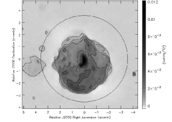
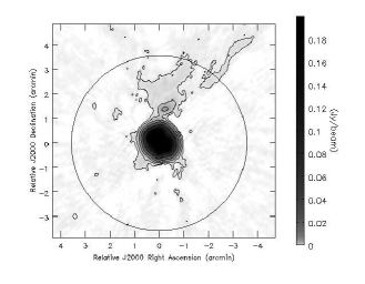
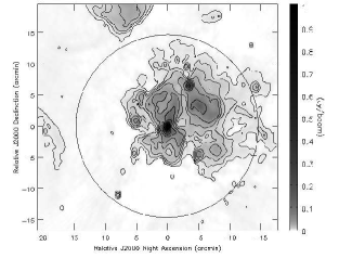
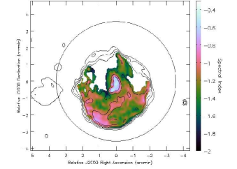
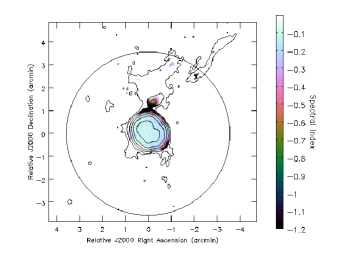
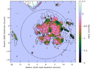
Figure 1.— Stokes-I (top row) and Spectral Index images (bottom row). The first two columns show C-Band images of the SNRs G16.7$+$0.1 and G21.5$-$0.9 respectively. The resolution in these images is 10″ and RMS noise is $11\mu Jy~{}beam^{-1}$ and $30\mu~{}Jy~{}beam^{-1}$ respectively. The last column shows the L-Band image of G19.6$-$0.2 with a compact source of thermal emission of positive spectral index surrounded by non-thermal emission with a negative spectral index. The resolution in this image is 40″ and RMS noise of $0.2m~{}Jy~{}beam^{-1}$. The circle indicates the half-power point of the antenna primary beam at the reference frequencies of 6.0 GHz for C-Band images and 1.5 GHz for the L-Band image.

4.1. G16.7$+$0.1, G21.5$-$0.9, G19.6$-$0.2

Figure 1 shows the Stokes-I and Spectral Index images of two catalogued SNRs (G16.7$+$0.1 and G21.5$-$0.9) (Green, 2009) and one candidate SNR (G19.6$-$0.2). The top row shows the Stokes-I images and the bottom row shows the spectral index images, with the Stokes-I contours overlaid on the spectral images. Correction for the primary beam response raises the noise away from the center. In order to show the detailed brightness distribution, we chose to show the Stokes-I images without correcting for the primary beam response. The integrated flux reported below was determined from PB-corrected images. The spectral index images have been corrected for the average primary beam effects, since the effect of primary beam response in the spectral index images is stronger. Image of all the fields covering the full wide-band sensitivity show many more compact and diffused sources. Due to space limitation, here we show central portions of these images.

The first column has the images at a reference frequency of 6 GHz, of the composite SNR G16.7$+$0.1 at a resolution of 10″. The SNR has a flatter spectrum core with an average spectral index of $-0.54\pm 0.02$ ($S\propto\nu^{\alpha}$) surrounded by a relatively steeper spectrum nebula with the spectral index ranging from $-0.8$ to $1.1$. The total continuum integrated flux is 1.2 Jy with an RMS noise of 11 $\mu~{}Jy~{}beam^{-1}$. The diffused sources on east of SNR are unrelated but real sources of emission. The images in the second column are of the filled-centered SNR G21.5$-$0.9, also at the reference frequency of 6 GHz. The RMS noise in this image is $\sim 30\mu~{}Jy~{}beam^{-1}$ and the resolution is 10″. The spectral index across this SNR is uniform across with a value of $+0.12\pm 0.03$ and integrated flux density of 6 Jy. Also visible in the image is the compact source called the “northern knot” about 2′ to the north. The long extended feature extending towards the north-west direction is part of the separate catalogued SNR G21.6$+$0.84. The third column contains the L-Band images at a reference frequency of 1.5 GHz, of the region centered on the Galactic co-ordinates $l=19.6^{\circ},b=-0.2^{\circ}$. This field contains a candidate SNR G19.66$-$0.22 (Helfand et al., 2006). Stokes-I image shown in the top row shows weak diffused emission surrounding two compact strong sources, making it difficult to determine the nature of the objects based on Stokes-I morphology alone. The spectral index image however clearly separates sources of thermal and non-thermal emission. The spectral index of the diffused emission range from $-0.4$ to $-0.5$. The spectral index of the compact source (G19.67$-$0.15) towards the norther edge of the diffused nebula has a spectral index of $-0.3$. The superimposed compact thermal source near the center is the known ultra-compact H ii region G19.61$-$0.23 (e.g., Wood & Churchwell (1989); Hofner & Churchwell (1996)) also with a spectral index of $+0.3$. Based on morphology of the spectral distribution we conclude that this field contains an SNR, possibly of filled-centered type.

4.2. G55.7$+$3.4

The SNR G55.7+3.4 is classified as an “incomplete-shell SNR” with a pulsar within the boundary of the remnant based on the only existing radio image at 610 and 1.415 GHz by Goss et al. (1977). These are the only image published in the literature of this SNR made over three decades ago using the Westerbork Synthesis Radio Telescope. The full $2^{\circ}\times 2^{\circ}$ Stokes-I L-Band image centered on this SNR at the reference frequency of 1.5 GHz covering the full wide-band sensitivity pattern of the EVLA antenna is shown in Figure 2. This is the highest resolution and sensitivity image of this region to date. The wide-band sensitivity pattern of the EVLA extended significantly beyond even the first sidelobe of the PB at the lowest frequency in the band. The time-averaged wide-band sensitivity pattern of the EVLA for the equivalent frequency range and field-of-view is shown in the left panel of Figure 3. The one-dimensional slice through this pattern in the right panel, shows the sensitivity pattern extending significantly beyond the “main-lobe” at the level of $5-15\%$ of the peak value. With sources, some strong, detected up to $1^{\circ}$ away from the center of the image, imaging the full field was required to reach noise-limited imaging at the center of the field. Due to this wide field of view, even for D-array observations, correction for the effects of non-coplanar baselines had to be applied. This was done using the W-Projection algorithm (Cornwell et al., 2008). The Stokes-I image of the SNR shows a nearly complete shell-type SNR. At a resolution of 30″, this image for the first time, shows a network of filamentary structures along with smoother diffused emission filling the boundary of the shell. The spectral index image of this SNR however was not reliable at all scales since the large scale emission is not well constrained by the shortest measured baselines at all frequencies. The filaments however show up as regions of steeper spectral index compared to an average spectral index of $-0.6$ of the surrounding regions. The strong compact source (G55.78$+$3.5) on the northern edge of the shell in the Stokes-I image is an older unrelated pulsar (PSR J1921$+$2153). In the spectral index map (not shown here), this pulsar shows up as a steep spectrum compact source with a spectral index of $-2.2$. The integrated flux of the shell, including the pulsar and other foreground or background sources superimposed across the shell is 1.0 Jy. The rms noise in the image is 10 $\mu Jy~{}beam^{-1}$.

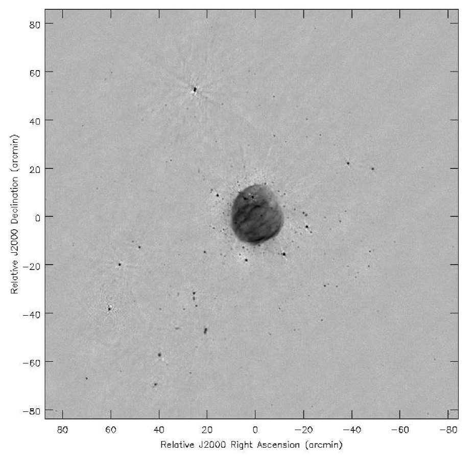
Figure 2.— Stokes-I image at a reference frequency of 1.5 GHz. Data in the frequency range 1.256–1.905 GHz were included for this image. For this frequency range, the HPBW of the primary beam changes from 32′ to 21′. This $2^{\circ}\times 2^{\circ}$ image covers the full-field corresponding to the wide-band sensitivity pattern of the EVLA (see Figure 3) of the field containing the SNR G55.7+3.4.

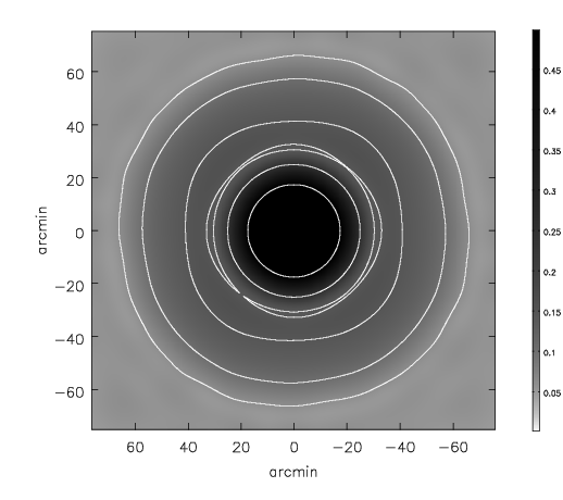
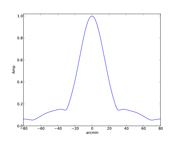
Figure 3.— The EVLA time-averaged wide-band sensitivity pattern covering the same frequency range and the area shown in Figure 2. The left panel shows the pattern in gray scale with overlaid contours at 50%, 25%, 15%, 10% and 6% of the peak value. The right panel shows a one-dimentional cut through the pattern shown on the left.

5. Discussion

The technical goals of this pilot project were to assess our low-frequency wide-band imaging capabilities for targets in the Galactic plane. At L-Band and C-band, the Galaxy is replete with compact and diffuse emission of both thermal and non-thermal origin. Sources often have a mixture of thermal and non-thermal emission, resulting in spectral indices that vary with position across a given source and with spatial scale. Conventional imaging algorithms that rely on multiple narrow-band images to derive spectral-index information are limited to the angular resolution allowed by the lowest measured frequency, and the single-channel sensitivity. The MS-MFS algorithm was designed to optimally use the multi-frequency measurements to do spectral-index mapping across diffused sources at the highest sensitivity and angular resolution offered by the data.

The following is a summary of our current status, based on the imaging results shown in the previous section. Our targets were chosen based on existing information about their spatial and spectral structure, in order to test the analysis methods in preparation for a Galactic plane survey.

1. Separation of thermal versus non-thermal; steep versus steeper spectra : we see clear morphological separations between regions expected to have different spectral structure from the surroundings. These differences range from $\triangle\alpha\approx 0.6$ between thermal and non-thermal regions, down to $\triangle\alpha\approx 0.2$ between structures thought to be cores and shells. In regions with high S/N ratios ($>100$), the estimated uncertainty in the spectral index is $\pm 0.03$. In regions with low signal-to-noise ($<100$), the uncertainty in the spectral index rises rapidly, and all the images presented here used a Stokes-I S/N threshold of 100.

2. Image-reconstruction errors : errors in the spectral reconstructions are dominated by multi-scale deconvolution artifacts that decrease with appropriate choices of multi-scale imaging parameters (a set of scale-sizes with which to model the spatial structure). Error estimates from Monte-Carlo simulations (by varying the choice of spatial scales) range from $\pm 0.02$ when scales are chosen appropriately, up to 0.2 in the extreme case where diffuse emission is modeled by a series of $\delta$-functions. These simulations were done for the EVLA D-configuration and the errors depend on the precise uv-coverage just as they depend for the standard imaging algorithms. The MS-MFS algorithm reconstructs the frequency dependence of the flux by a polynomial fit across the frequency range on a per component basis. The errors on the estimated spectral index therefore also depend on the errors of the fitted coeffcients. These errors depend on variations in S/N ratio (across the frequency range or due to the scale of the emission) in the same way as the errors on the coefficients of any least-squares polynomial fitting algorithm (see  Press et al. (2007); Rau & Cornwell (submitted,2011) for further details). Further, at the largest spatial scales sampled by the interferometer (which, of course, is telescope dependent), the spectrum is unconstrained by the data and the MS-MFS model does not provide adequate additional constraints. Out of our examples, G55.7$+$3.4 and G16.7$+$0.1 contain structure at spatial scales that fall within the unsampled central region of the interferometer sampling function, aleading to overall systematic errors in the spectral index across the source. These errors are limited to the largest scales, but in the current implementation of the algorithm, it is not possible to analyse the scales separately. In our examples, G55.7$+$3.4 is affected significantly by this error and spectra of only the most compact emission can be trusted. Finally, in addition to errors in the spectral index, off-source artifacts are present in the Stokes-I images beyond dynamic-ranges of a few thousand (measured as the ratio of the peak brightness to the peak residual near the source). Dynamic-ranges for the images presented here range from 2000 for G16.7$+$0.1 to 10000 for G19.6$-$0.2. In most cases, wide-band self-calibration was required to achieve these limits.

3. Wide-field wide-band sensitivity of the instrument, and related errors : across a 2:1 bandwidth, the size of the antenna power-pattern changes enough to produce an average beam that is significantly different from the beams at individual frequencies. The most-prominent difference is the near lack of a first null, with sensitivity at the few percent level out to almost three times the HPBW. The G55.7$+$3.4 field is an example of this wide-field sensitivity pattern (the reference-frequency primary beam has a HPBW of 30′). For sources far from the phase-center, the $w$-term causes the dominant wide-field error, and these images (in particular G55.7+3.4) are a result of W-Projection combined with MS-MFS. The next dominant error (in Stokes-I and spectral index) is due to the frequency dependence of the primary beam. All the spectral-index maps shown here have been corrected for this effect using the time-averaged PB-model, and can be trusted out to the 25% point of the reference-frequency primary-beam. The time-variability of the primary-beams has not been accounted for, and is thought to be the cause of the next dominant error (visible as artifacts around bright sources about $1^{\circ}$ from the phase center in G55.7$+$3.4).

The next steps in our analysis include combining multi-configuration and multi-band data for the G16.7$+$0.1 and G19.6$-$0.2 fields to introduce more constraints during image-reconstruction, to complete the software integration required to combine MS-MFS and W-Projection with the A-Projection algorithm to correct for time-varying primary-beams, and further tests with mosaicking observations and how the additional information aids the image reconstruction. These steps are in accordance with our long-term goal of doing a wide-band mosaiced survey of the Galactic plane at low frequencies.

References

- Bhatnagar & Cornwell (2004) Bhatnagar, S., & Cornwell, T. J. 2004, Astron. & Astrophys., 426, 747
- Bhatnagar et al. (2008) Bhatnagar, S., Cornwell, T. J., Golap, K., & Uson, J. M. 2008, Astron. & Astrophys., 487, 419
- Bietenholz et al. (2011) Bietenholz, M. F., Matheson, H., Safi-Harb, S., Brogan, C., & Bartel, N. 2011, MNRAS, 412, 1221
- Cornwell (2008) Cornwell, T. J. 2008, IEEE Journal of Selected Topics in Signal Processing, issue 5,, 2, 793
- Cornwell et al. (2008) Cornwell, T. J., Golap, K., & Bhatnagar, S. 2008, IEEE JSTSP, 2, 647
- Goss et al. (1977) Goss, W. M., Schwartz, U. J., Siddesh, S. G., & Weiler, K. W. 1977, Astron. & Astrophys., 61, 93
- Green (2009) Green, D. A. 2009, Bulletin of the Astronomical Society of India, 37, 45
- Gupta et al. (2005) Gupta, Y., Mitra, D., Green, D. A., & Acharyya, A. 2005, Current Science, 89, 853
- Helfand et al. (2006) Helfand, D. J., Becker, R. H., White, R. L., Fallon, A., & Tuttle, S. 2006, Astron. J., 131, 2525
- Helfand et al. (1989) Helfand, D. J., Velusamy, T., Becker, R. H., & Lockman, F. J. 1989, ApJ, 341, 151
- Hofner & Churchwell (1996) Hofner, P., & Churchwell, E. 1996, Astron. & Astrophys. Suppl. Ser., 120, 283
- Manchester et al. (2005) Manchester, R. N., Hobbs, G. B., Teoh, A., & Hobbs, M. 2005, AJ, 129, 1993
- Press et al. (2007) Press, W. H., Teukolsky, S. A., Vetterling, W. T., & Flannery, B. P. 2007, Numerical Recipes (3rd Edition), The Art of Scientific Computing (Cambridge University Press)
- Rau (2010) Rau, U. 2010, PhD thesis, The New Mexico Institute of Mining and Technology, Socorro, New Mexico, USA
- Rau & Cornwell (submitted,2011) Rau, U., & Cornwell, T. J. 2011,Astron. & Astrophys., (accepted)
- Slane et al. (2000) Slane, P., Chen, Y., Schulz, N. S., Seward, F. D., Hughes, J. P., & Gaensler, B. M. 2000, ApJ, 533, L29
- Wood & Churchwell (1989) Wood, D. O. S., & Churchwell, E. 1989, AJ Supp., 69, 831