The nearby eclipsing stellar system $\delta$ Velorum

Abstract

Context. The triple stellar system $\delta$ Vel (composed of two A-type and one F-type main sequence stars) is particularly interesting as it contains one of the nearest and brightest eclipsing binaries. It therefore presents a unique opportunity to determine independently the physical properties of the three components of the system, as well as its distance.

Aims. We aim at determining the fundamental parameters (masses, radii, luminosities, rotational velocities) of the three components of $\delta$ Vel, as well as the parallax of the system, independently from the existing Hipparcos measurement.

Methods. We determined dynamical masses from high-precision astrometry of the orbits of Aab-B and Aa-Ab using adaptive optics (VLT/NACO) and optical interferometry (VLTI/AMBER). The main component is an eclipsing binary composed of two early A-type stars in rapid rotation. We modeled the photometric and radial velocity measurements of the eclipsing pair Aa-Ab using a self consistent method based on physical parameters (mass, radius, luminosity, rotational velocity).

Results. From our self-consistent modeling of the primary and secondary components of the $\delta$ Vel A eclipsing pair, we derive their fundamental parameters with a typical accuracy of 1%. We find that they have similar masses, respectively $2.43\pm 0.02$ $M_{\odot}$ and $2.27\pm 0.02$ $M_{\odot}$. The physical parameters of the tertiary component ($\delta$ Vel B) are also estimated, although to a lower accuracy. We obtain a parallax $\pi=39.8\pm 0.4$ mas for the system, in satisfactory agreement ($-1.2\,\sigma$) with the Hipparcos value ($\pi_{\rm Hip}=40.5\pm 0.4$ mas).

Conclusions. The physical parameters we derive represent a consistent set of constraints for the evolutionary modeling of this system. The agreement of the parallax we measure with the Hipparcos value to a 1% accuracy is also an interesting confirmation of the true accuracy of these two independent measurements.

1 Introduction

Early-type main sequence stars exhibit a number of peculiarities usually not encountered in cooler stars: fast rotation, debris disks, enhanced surface metallicities (Am), magnetic fields and rapid oscillations (Ap and roAp stars), etc. Although stellar structure and evolution models are now rather successful in reproducing the observed physical properties of most A-type stars, the observational constraints on these models remain relatively weak, occasionally leading to surprising discoveries. An example is provided by the recent interferometric observations of the A0V benchmark star Vega, that confirmed that Vega, as previously shown by Gulliver, Hill & Adelman (gulliver94 (1994)), is a pole-on fast rotator near critical velocity (Aufdenberg et al. aufdenberg06 (2006)). The same interferometric observations showed that Vega harbors a hot debris disk within within 8 AU from the star (Absil et al. absil06 (2006)).

$δ$ Vel (HD 74956, HIP 41913, GJ 321.3, GJ 9278) is a bright multiple star including at least three identified components, and is among our closest stellar neighbors, with a revised Hipparcos parallax of $\pi_{\rm Hip}=40.5\pm 0.4$ mas (van Leeuwen vanleeuwen07 (2007)). This object has many observational peculiarities. Firstly, it was discovered only in 1997 that $\delta$ Vel hosts one of the brightest of all known eclipsing binaries (Otero et al. otero00 (2000)), with a remarkably long orbital period ($P\approx 45$ days). This eclipsing binary is also one of the very few that are easily observable with the naked eye ($m_{V}\approx 2$). The eclipsing pair was first resolved using optical interferometry by Kellerer et al. (kellerer07 (2007)). Secondly, $\delta$ Vel is known to have a moderate thermal infrared excess (e.g. Aumann aumann85 (1985), Su et al. su06 (2006)), and Spitzer observations revealed a spectacular bow shock caused by the motion of $\delta$ Vel in a dense interstellar cloud (Gáspár et al. gaspar08 (2008)). The presence of interstellar material was also reported by Hempel & Schmitt (hempel03 (2003)), who observed two red-shifted absorbing components in absorption in the Ca II K line, of probable interstellar origin. In Paper I of the present series, Kervella et al. (kervella09 (2009)) confirmed that the infrared excess is essentially emitted by the bow shock, and not warm circumstellar material located close to the stars. In the framework of a search for resolved emission due to debris disks, Moerchen et al. (moerchen10 (2010)) obtained thermal infrared images of $\delta$ Vel using the Gemini South telescope and the T-ReCS instrument, and detected a marginally resolved emission at $\lambda=10.4\,\mu$m.

In Paper II, Pribulla et al. (pribulla11 (2011)) used a combination of high-resolution spectroscopy and photometric observations (from the SMEI instrument, attached to the Coriolis satellite) to derive an accurate orbital solution for the eclipsing binary $\delta$ Vel A, and estimate the physical parameters of $\delta$ Vel Aa and Ab. They identified that the two eclipsing components are fast rotating stars, with respective masses of $2.53\pm 0.11\,M_{\odot}$ and $2.37\pm 0.10\,M_{\odot}$ ($\approx 4\%$ accuracy), and estimated the mass of $\delta$ Vel B to be $\approx 1.5\,M_{\odot}$.

In spite of this recent progress, uncertainties remain on the fundamental parameters of the different components of the system, in particular on their exact masses. Taking advantage of the availability of NACO astrometry of the $\delta$ Vel A-B pair, and new interferometric observations from the VLTI/AMBER instrument, we propose here to revisit the system along two directions. In Sect. 2, we describe our new VLTI/AMBER interferometric data, as well as our re-analysis of the spectroscopic and photometric data previously used in Paper II. Sect. 2.2 is dedicated to the description of our self-consistent model, and the derivation of an improved orbital solution, physical parameters as well as an independent distance. In Sect. 3 we employ NACO astrometry of the visual $\delta$ Vel A-B binary to obtain an improved orbital solution. Compared to our work presented in Paper II, this new analysis result is a clearer view and better confidence in the derived fundamental parameters of the system (for all three components), thanks to the redundant nature of our data and our independent determination of the distance.

2 The orbit and parameters of $\delta$ Vel Aa and Ab

2.1 Observations and data analysis

2.1.1 Interferometry

AMBER (Petrov et al. petrov07 (2007)), the three-telescope beam combiner of the VLTI, has the proper angular resolution to resolve the Aa-Ab pair. This instrument combines simultaneously 3 ATs (Auxiliary Telescopes) or 3 UTs (Unit Telescopes) of the VLT and operates in the near infrared (H and K band). It has a choice of spectral resolutions of $R\sim 35$, $R\sim 1500$ or $R\sim 15000$. For this study, we had data in low resolution (H+K bands at $R\sim 35$) and medium resolution (H or K band, at $R\sim 1500$). We used baselines of the order of 100 m in order to obtain spatial resolution in the milli-arcsecond regime. These interferometric data have been collected in a dedicated program (ESO program 076.D-0782), as well as during Guaranteed Time (GTO) from Arcetri Observatory. We present here a reduction of these data.

We reduced the data using the AMBER reduction package amdlib3 (Chelli et al. chelli09 (2009), Tatulli et al. tatulli07 (2007)) and performed the calibration using stellar calibrators chosen in the catalogue by Mérand et al. (merand05 (2005)) and a custom software which estimates and interpolates the transfer function of the instrument. For each night, we derived the separation of Aa and Ab using a $\chi^{2}$ map as a function of the separation vector (two parameters). The other parameters, such as flux ratio or individual diameters, were set using simple hypothesis and their choice did not affect significantly our final estimated angular separations. The resulting separation vectors are listed in Table 1 in coordinate towards East and North (which correspond to the $u$ and $v$ axes in the projected baselines map). The error bars on this vectors were estimated in the $\chi^{2}$ map.

Table 1: AMBER separation vectors (primary to secondary)

date	toward East	toward North
MJD	mas	mas
53427.09	$-4.1\pm 0.4$	$7.3\pm 0.5$
53784.08	$-6.5\pm 0.5$	$13.8\pm 0.3$
54819.25	$-7.3\pm 0.2$	$16.1\pm 0.2$
54832.12	$2.7\pm 0.7$	$-6.4\pm 0.4$
55147.38	$1.6\pm 0.5$	$-4.0\pm 0.5$

2.1.2 Photometry

We used the photometric data from the SMEI satellite, presented in Paper II. The available quantity is the relative flux normalized to the value outside of the eclipses, since there was no absolute calibration of SMEI data available. We corrected for the presence of the B component which is in the field of view of SMEI. From our model of B, the expected flux ratio between B and Aab is 7.5% in the SMEI bandpass. The transmission of the instrument has a triangular shape that peaks at 700 nm, with a quantum efficiency around 47%, and falls to $\approx 5\%$ at 430 nm towards the blue, and 1025 nm towards the red (Spreckley & Stevens spreckley08 (2008)). We removed this contribution which, if not taken into account, would result in an underestimation of the depth of the eclipses. We also incorporated to our photometric dataset the photometric measurement we derived of Aab in the K band (Paper I). We use this value in our fit as the only constraint in term of absolute photometry.

2.1.3 Spectroscopy

The observables we derived from the visible spectroscopic data are the broadening functions (BF) presented in paper II (see this reference for more explanations). These functions contain a lot of information: not only do they contain the radial velocities that result from the orbital motion, but also the broadening due to the stellar rotation and the flux ratio in the considered band.

From the observed BF, it is possible to derive the $v\sin i$ from the two components. After a few experimentations using the stellar surface model we are going to present later, we found that the following ad-hoc function parameterizes well the BF for a star seen from the equator:

$$\frac{\mathrm{BF}(v)}{\mathrm{BF}(v_{0})}=\left(1-\cos\left(\left[1-\left(\frac{v-v_{0}}{v\sin i}\right)^{2}\right]\times\pi/2\right)\right)^{\alpha}$$ (1)

where $\alpha$ is the only parameter constraining the gravity darkening and $v_{0}$ is the velocity offset. The function is defined for $|v-v_{0}|\leq v\sin i$ only, and its value is 0 otherwise. Using this analytical model and a global fit, we estimated $v\sin i$ for each component and the radial velocities for each epoch (see Fig. 1 and 2 for the quality of the fit). We found $v\sin i$ to be $143.5\pm 0.2$ km/s and $149.6\pm 0.2$ km/s for Aa and Ab respectively. Incidentally, we find $\alpha_{a}=0.460\pm 0.003$ and $\alpha_{b}=0.451\pm 0.003$. The rotation rate value is relatively independent of the actual gravity darkening (parameterized here by $\alpha$) since it is set by the width of the broadening function, not its shape.

For our fit of the orbit and the stellar parameters, we do not use the center-to-limb darkening we derive here from the broadening functions. The surface brightness distribution is constrained by the photometric profil of the eclipses. However, we will check a posteriori the agreement between our best fit model and the limb-darkening derived in the analytical BF by modeling the BF from our model. See Sect. 2.2.3 and, more specifically, Fig. 7.

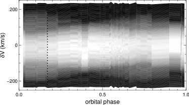
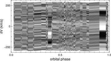
Figure 1: $\delta$ Vel Aa-Ab spectroscopic broadening functions (BF). Upper: BF as a function of orbital phase; Lower: residuals after the fit. See Fig. 2 for the fit at the phase corresponding to the dotted line ($\phi\approx 0.17$). Our method to extract the radial velocity does not take into account the eclipses, as can be seen by the large residuals during the eclipses ($\phi\approx 0.40$ and $\phi\approx 0.97$, upper right panel).

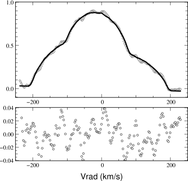
Figure 2: Example of one fit of a broadening function (for the phase represented as a dotted line in Fig. 1, $\Phi\approx 0.17$). The analytical fit uses the sum of two functions described in eq. 1.

2.2 Global fit

2.2.1 Self consistent model

In order to extract the fundamental parameters (masses, radii, surface temperatures, semi-major axis, etc.) from the observational data, we propose a self consistent modeling centered around the use of physical quantities: we model the system using two stars whose characteristics are computed based on their radii, total luminosities and mass.

To illustrate the advantage of this approach, we can consider that in order to model the eclipses, we could use an ad-hoc model based on fractional radii (ratio to the semi-major axis) and brightness ratio, but this would not lead directly to the fundamental parameters of the system such as effective temperatures or luminosities. Our approach uses radii, masses and luminosities: we get the fractional radii by self consistency between the semi-major axis based on Newton’s form of the Kepler’s law (from the masses and the period of the orbit) and the measured apparent semi-major axis (constrained by interferometric separation vectors). The brightness ratio arises from the luminosity and radii, and the photospheric models we use to model the surface of the stars.

Our stellar surface model also includes stellar rotation. We model the appearance of the star using a model developed contemporarily and similar to the one used in Aufdenberg et al. (aufdenberg06 (2006)) to model the interferometric visibilities of the star Vega. To compute the photometry, in particular during the eclipses, we generated synthetic images and integrated them to derive the light curves. The parameters we use are:

• total mass of the system (Aa+Ab);

• the fractional mass of Aa to the total mass of the eclipsing system (Aa+Ab);

• the physical radii of each component;

• the absolute luminosity of each component;

• the $v\sin i$ of each component, to parameterize the rotation;

In addition, we have the usual 7 parameters for the visual orbit:

• the period;

• the date of passage at periastron;

• the eccentricity;

• three angles: inclination, $\omega$ and $\Omega$;

• the apparent semi-major axis (in milliarcseconds)

The only parameterization of the physics of the two components is contained in the luminosity: the model we use of the stellar surface is the Roche approximation, which only uses the mass, radius, luminosity and rotational velocity. Once the shape of the surface is computed, we link the local surface gravity and local effective temperature using the von Zeipel theory (von Zeipel vonzeipel24 (1924) and Aufdenberg et al. aufdenberg06 (2006) for more details). The luminosity is constrained using several mechanisms: through the absolute photometry of the system, but also through the surface brightness that sets the depth of the eclipses.

The advantages of using the apparent semi-major axis compared to the physical quantity are simple. First of all, it is directly related to one of our observables: the interferometric separation vector. Secondly, we already have the semi-major axis by combining the Kepler’s third law, the period and the total mass. Combined with the angular semi-major axis, we derive a distance independently from the Hipparcos value (a brief discussion is presented in Sect. 2.3). The distance is derived internally in our model and used to extract a model apparent magnitude in the K band, which is used as one of the constraints as we mentioned before.

It is to be noted that we make the following assumptions:

• the stars have their rotation axis perpendicular to the plane of the orbit.

• we use a Von Zeipel gravity darkening coefficient of $\beta=0.25$ in $T_{\mathrm{eff}}\propto g_{\mathrm{eff}}^{\beta}$, where $T_{\mathrm{eff}}$ and $g_{\mathrm{eff}}$ are the effective temperature and gravity at the surface. Even if recent observational constraints from Monnier et al. (monnier07 (2007)) suggest $\beta\approx 0.19$, we chose to use von-Zeipel’s classical value since it does not lead to qualitatively nor quantitatively different results in our case.

2.2.2 Orbital and stellar derived parameters

The result of the global fit is in excellent agreement with all the observed data we used for the fit: the relative photometry of the eclipses (Fig. 3 and 4), the radial velocities (Fig. 5) and the separation vectors (Fig. 6). The corresponding orbital parameters and stellar parameters are presented in Tables 2 and 3.

Table 2: Aa-Ab orbital and stellar parameters fitted on the photometric, interferometric and radial velocity data, using our model.

	Aa	Ab	constrained from
$a$ (mas)	$16.51\pm 0.16$		interferometry
Total mass ($M_{\odot}$)	$4.69\pm 0.03$		all observations
$M_{\mathrm{Aa}}/(M_{\mathrm{Aa}}+M_{\mathrm{Ab}})$	$0.516\pm 0.001$		spectroscopy
Polar Radius ($R_{\odot}$)	$2.79\pm 0.04$	$2.37\pm 0.02$	photometry
Luminosity ($L_{\odot}$)	$67\pm 1$	$51\pm 1$	photometry
$v\sin i$ (km/s)	$143.5\pm 0.2$	$149.6\pm 0.2$	spectroscopy
Period $P$ (d)	$45.1503\pm 0.0002$		all observations
MJD0 modulo $P$	$19.159\pm 0.010$		all observations
$e$	$0.287\pm 0.001$		all observations
$i$ (deg)	$89.04\pm 0.03$		all observations
$\omega$ (deg)	$109.79\pm 0.09$		all observations
$\Omega$ (deg)	$65.0\pm 0.6$		interferometry
$V_{\gamma}$ (km/s)	$-9.78\pm 0.07$		spectroscopy
$\chi^{2}$ $V_{\mathrm{rad}}$ Primary (err 0.75km/s)	$1.13$
$\chi^{2}$ $V_{\mathrm{rad}}$ Secondary (err 1.3km/s)	$1.03$
$\chi^{2}$ Photometry (err 0.75%)	$1.15$
$\chi^{2}$ Interferometry	$1.05$

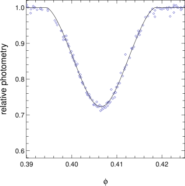
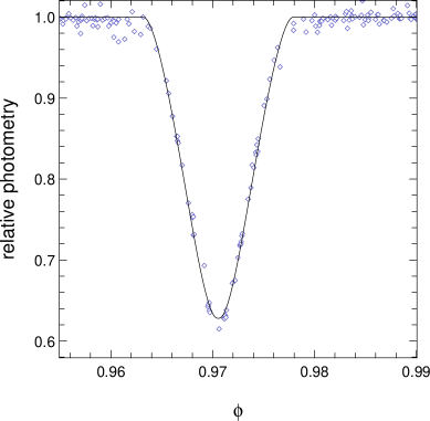
Figure 3: $\delta$ Vel Aa-Ab SMEI photometric measurements (points) and fit of the eclipses (line) as a function of orbital phase: the upper panel is the the primary eclipse, the lower panel the secondary.

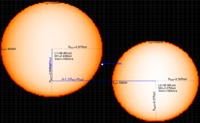
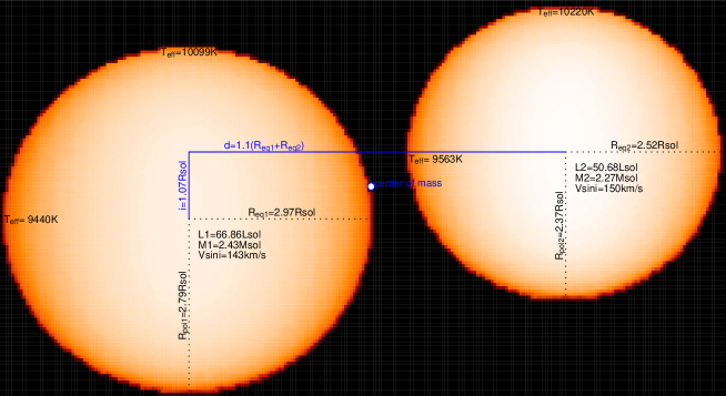
Figure 4: $\delta$ Vel Aa-Ab synthetic images in linear scale, close to the eclipses: the upper panel is the configuration of the primary eclipse, the lower panel is the secondary eclipse.

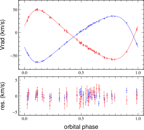
Figure 5: $\delta$ Vel Aa-Ab radial velocities as a function of orbital phase, with model from the fit over plotted and residuals plotted in the lower panel. Round points (blue) are for the primary and diamonds (red) for the secondary.

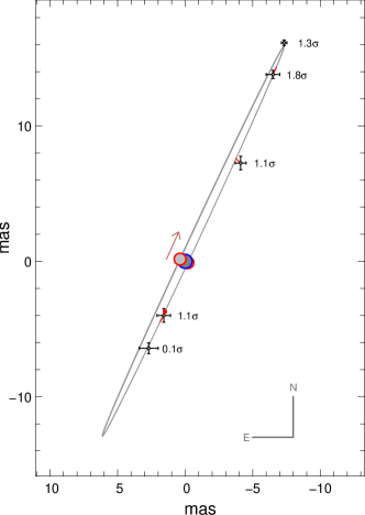
Figure 6: $\delta$ Vel Aa-Ab visual orbit: AMBER positions (black dots with error bars, see Table 1); fitted orbit (gray line), Aa stellar disk (dark gray disk with blue surrounding), the position of Ab at periastron (red dot) and Ab stellar disks for the positions of the eclipses (gray disk with red surroundings). Residuals to the orbit (red lines, too small to see in most cases) and quality of the fit (in number of sigmas). The overall agreement corresponds to a reduced $\chi^{2}$ of 1.05.

Table 3: Derived fundamental parameters for $\delta$ Vel Aa and Ab.. Parameters for Vega are displayed for comparison.

	unit	$\delta$ Vel Aa	$\delta$ Vel Ab	Vega
Mass	$M_{\odot}$	$2.43\pm 0.02$	$2.27\pm 0.02$	$2.3\pm 0.2$
Luminosity	$L_{\odot}$	$67\pm 3$	$51\pm 2$	$37\pm 3$
Polar Radius	$R_{\odot}$	$2.79\pm 0.04$	$2.37\pm 0.02$	$2.26\pm 0.07$
Equ. Radius	$R_{\odot}$	$2.97\pm 0.02$	$2.52\pm 0.03$	$2.78\pm 0.02$
Polar $T_{\mathrm{eff.}}$	K	10100	10120	10150
Equ. $T_{\mathrm{eff.}}$	K	9700	9560	7900
Avg. $T_{\mathrm{eff.}}$	K	9450	9830	9100
$\omega/\omega_{\mathrm{crit.}}$		0.61	0.60	0.91
Polar $\log(g)$	cm s-2	3.90	4.10	$4.10\pm 0.1$
Eq. $\log(g)$	cm s-2	3.78	3.99	$3.65\pm 0.1$
$i$	deg	$\sim 90$	$\sim 90$	$4.7\pm 0.3$
rotation rate	1/d	0.95	1.17	1.90
metallicity	[M/H]	$-0.33^{1}$	$-0.33^{1}$	$-0.5^{2}$

2.2.3 a posteriori verifications

Our model is rather simple and does not take into account one aspect: the heating of one star by the other’s radiation. This effect could be important in our case in different conditions. The first one is if one star was heated by the other one and developed a bright spot on its surface. We can discard this possibility because of the absence of photometric variations outside the eclipses. The second case where the heating by the other star can be a problem is if this contribution is enough to actually modify the temperature structure of the stellar photosphere. We can check a posteriori that the radiation received from the other star is of the order of 3% of the radiation emitted (assuming similar surface brightness and a 2.5 $R_{\odot}$ star seen at a distance of 89 $R_{\odot}$). Approximating the surface as a blackbody, it corresponds to an increase of temperature of less than 1% ($1.03^{1/4}$). We can thus assume that our hypothesis that locally the photosphere can be approximated by a ATLAS model is correct.

We can also check the consistency of our model beyond the fit of the data we presented. In particular, we can compare the predicted broadening functions based on our model and the broadening functions we observe since we did not implement the direct fit of broadening function to our model. Doing so (Fig. 7), the comparison is very satisfactory, even though the wings of the data (represented by the analytical function fit to the data in thick gray line) seems deeper than for the model. In other words, the gravity darkening of the model is slightly underestimated, but only by a small fraction, considering that a model without gravity darkening (small gray dots on Fig. 7) produces a very strong disagreement.

Investigating the possible causes of this problem, we realized that we can reproduce the more pronounced darkening of the equator compared to the pole by tilting the star to 10 degrees from the plane of the sky: this makes the pole more in line of sight of the observer and hence increases the contrast between the pole and the equator.

Forcing the inclination of the spin of the stars to be 80 degrees instead of 90 degrees does not change dramatically the fundamental parameters of the star estimated from our fit. One of the reasons is that it changes the sin(i) by only 1.5%, the actual rotational velocity is mostly unaffected. The fit converges as well as in the case of aligned spins, with fundamental parameters within error bars of the one estimated in the case we presented in the main part of this work.

In conclusion of the analysis of the broadening function prediction of our model compared to the observed one, we find a confirmation of the consistency of our model with the data. This comparison may also indicate that our model underestimate slightly the gravity darkening, or, alternatively, that the stars have their rotational axis tilted on the order of 10 degrees toward the observer, which does not impact qualitatively nor quantitatively the fit of the data that led to the estimation of the fundamental parameters presented earlier.

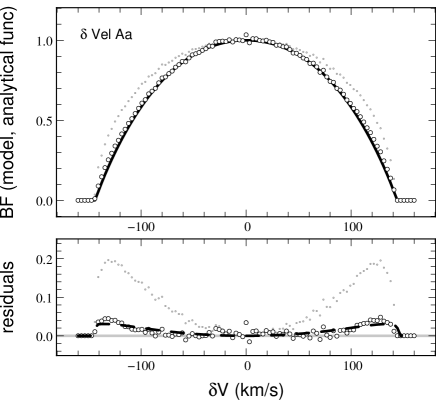
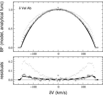
Figure 7: $\delta$ Vel Aa-Ab expected broadening functions computed for our models. For each star (Aa and Ab), the open dots are for the model (Table 3) and the thick line is for the analytical function resulting from the fit to the spectroscopic data (Fig. 2). The small gray dots are for the model as well, but ignoring the gravity darkening. In the smallest panels are plotted the residuals “model” - ”fit on spectroscopic data”, with the dashed line being the best fit on the model using the same analytical function, showing the slight underestimation of the gravity darkening by our model.

Another test is to compare the predicted wide band photometry with the observed ones. In the literature, there is a handful of data available, for the combined AB or A and B separately. Doing so, we see (Table 4) that the bluest magnitudes are not reproduced well. Assuming a $B-V$ excess of $E(B-V)=0.055$, the difference is nicely explained using an ISM extinction law as presented in Kervella et al. (kervella04 (2004)).

Table 4: Computed and observed broad band photometry.

	model (observation)					$\Delta$	extinction
band	Aa	Ab	Aab	B	AB	obs.-mod.	$E(B-V)=0.055$
B	2.39	2.71	1.78	6.10	1.76 (2.001)	0.24	0.23
V	2.41	2.73	1.81	5.59 (5.542)	1.78 (1.961)	0.18	0.18
J	2.43	2.76	1.83	4.72	1.76 (1.773)	0.02	0.04
H	2.45	2.78	1.85	4.44	1.75 (1.763)	0.01	0.03
K	2.46	2.78	1.85 (1.862)	4.42 (4.402)	1.76 (1.723)	-0.04	0.02

2.3 Distance

Our parameterization allows us to derive the distance as the ratio between of the semi-major axis of the eclipsing component (from the total mass, the period and Kepler’s third law) and its apparent semi-major axis (from the interferometric observations). Such a distance estimate is particularly interesting as it is purely geometrical, and independent of the Hipparcos measurement. From our model, we obtain a parallax of $\pi=39.8\pm 0.4$ mas for $\delta$ Vel.

Comparing this value to the $\pi_{\rm Hip}=40.5\pm 0.4$ mas revised Hipparcos parallax obtained by van Leeuwen (vanleeuwen07 (2007)) shows a good agreement of the two measurements, within $1.2\,\sigma$. This confirmation of the true accuracy of these independent measurements, at the 1% level, shows that the Hipparcos measurement was not disturbed by the binary nature of $\delta$ Vel A. This somewhat surprising result is due to the similar brightness ratio $L_{\mathrm{Aa}}/L_{\mathrm{Ab}}\approx 1.3$ and mass ratio $M_{\mathrm{Aa}}/M_{\mathrm{Ab}}\approx 1.1$ of the $\delta$ Vel A pair. This results in a very small apparent displacement of the center of light of the Aab system during the orbit, with respect to the center of gravity of the two stars. Using our model of the eclipsing system, we computed the expected photocenter displacement during an full orbit. We find that the peak-to-peak photocenter displacement is of the order of one milliarcsecond, which is much smaller than the apparent astrometric shift due to the parallax. The binarity of the system therefore did not bias significantly the Hipparcos parallax measurement, neither did the low brightness of the B component. The observations of the photocenter displacement through high-precision differential astrometry with the VLT/NACO instrument will be the subject of a future article.

3 The orbit and parameters of $\delta$ Vel B

3.1 Astrometric data

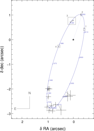
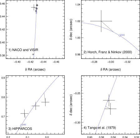
Figure 8: left panel: Astrometric measurements of the relative position of $\delta$ Vel B (crosses) with respect to $\delta$ Vel A ($\star$ symbol), with our best fit orbital solution (solid ellipse, see Table 6 for the orbital parameters). Thin lines connect each measurement to the corresponding point on the adjusted orbit. The dotted line corresponds to periastron passage, and the diamonds corresponds to the position of $\delta$ Vel B on Jan. $1^{\mathrm{st}}$ every ten years between 1890 and 2020. Right pannels (labeled 1 to 4): corresponds to zooming boxes on the larger view. NACO and VISIR data (panel 1) are tabulated in Table 5; data in panel 2 comes from Horch, Franz & Ninkov (Horch00 (2000)); data in panel 4 are from Tango et al. (tango79 (1979)). Zooming boxes’ positions are reported on the main (left) panel.

The binarity of $\delta$ Vel was discovered by S. I. Bailey in 1894 from Arequipa, Peru (and independently by Innes innes1895 (1895)). Over more than one century, the separation between $\delta$ Vel A and B has been decreasing at a rate which nicely matches the progression of the angular resolution of the successive generations of imaging instruments (visual observations, photography, electronic devices). This progression allowed a relatively regular tracing of the visual orbit of the pair, down to the sub-arcsecond separations that occur around the periastron passage. With the advent of speckle interferometry (Tango et al. tango79 (1979)) and the Hipparcos satellite (ESA esa97 (1997)) the accuracy of the measured relative positions improved significantly. In Paper I, we present in details the new data we obtained with the Very Large Telescope, using both the K-band adaptive optic system VLT/NACO (Rousset et al. rousset03 (2003); Lenzen et al. lenzen98 (1998)) and the N-band camera VLT/VISIR (Lagage et al. lagage04 (2004)). Thanks to the large aperture of the telescopes and the diffraction-limited angular resolution, these observations provide us with new high-precision astrometry of the A-B pair. The resulting separations of $\delta$ Vel B relatively to A are presented in Table 5. For the conversion of the separation measured in pixels to angular separations, we adopted the pixel scale of $13.26\pm 0.03$ mas/pixel (Masciadri et al. masciadri03 (2003)) for NACO and $75\pm 1$ mas/pixel for VISIR. The assumed NACO plate scale is in good agreement with the calibration by Neuhäuser et al. (neuhauser08 (2008)), who demonstrated that this figure is stable over a period of at least 3 years. The VISIR plate scale uncertainty is set arbitrarily to $\approx 1\%$, although it is probably better in reality. The angular separation was only $\approx 0.6\arcsec$ for the epoch of our observations.

In addition to these new astrometric measurements, we also take advantage of the historical astrometric positions assembled by Argyle et al. (argyle02 (2002)) in his Table 5, that includes 17 epochs between 1895 and 1999. It is to be noted that these authors used the two speckle interferometry epochs from Tango et al. (tango79 (1979)) with a different definition for the projection angle, leading to an apparent inconsistency with the other measurements. Transforming the Tango et al. projection angle $PA$ using $PA\rightarrow(180-PA)$, these two data points become much more consistent with the other epochs and observing techniques.

Table 5: Differential astrometry of $\delta$ Vel from NACO and VISIR images.

UT date	MJD-54 000	$[\alpha_{B}-\alpha_{A}]$	$[\delta_{B}-\delta_{A}]$
		mas	mas
2008-04-01N	557.0224	$-430.6\pm 1.0$	$457.8\pm 1.0$
2008-04-04N	560.9976	$-430.7\pm 1.0$	$457.1\pm 1.0$
2008-04-06N	562.0121	$-430.8\pm 1.0$	$457.1\pm 1.0$
2008-04-07N	563.0048	$-430.7\pm 1.0$	$457.0\pm 1.0$
2008-04-20N	576.9715	$-430.3\pm 1.0$	$452.9\pm 1.0$
2008-04-23N	579.0231	$-430.0\pm 1.0$	$452.0\pm 1.0$
2008-04-24V	580.0503	$-425.9\pm 4.3$	$454.0\pm 4.5$
2008-04-24N	580.9917	$-429.8\pm 1.0$	$451.1\pm 1.0$
2008-05-05N	591.9748	$-428.9\pm 1.0$	$448.7\pm 1.0$
2008-05-07N	593.9732	$-429.2\pm 1.0$	$448.0\pm 1.0$
2008-05-18N	604.0442	$-429.6\pm 1.0$	$445.4\pm 1.0$
2009-01-07N	838.1347	$-424.6\pm 1.0$	$381.3\pm 0.9$

3.2 Orbital elements

We adjusted the orbital parameters of the $\delta$ Vel A-B pair to the whole sample of astrometric data, and the result is presented graphically in Fig. 8. The corresponding orbital elements are listed in Table 6. It should be noted that thanks to a semi-major axis twice more precise, and a period ten time more precise, the total mass value derived from based Kepler’s third law is significantly improved, which becomes limited by our parallax estimation of $\pi=39.8\pm 0.4$.

$$M(\mathrm{Aab+B})=6.15\pm 0.15_{\mathrm{orbit}}\pm 0.17_{\mathrm{parallax}}\,M_{\odot}$$ (2)

Table 6: Orbital parameters of the visual pair A-B.

parameter	this work	Argyle et al. (argyle02 (2002))
$a$ (′′)	$1.996\pm 0.012$	$1.990\pm 0.020$
$e$	$0.475\pm 0.003$	$0.470\pm 0.020$
Period (yr)	$143.2\pm 1.2$	$142\pm 13$
$\mathrm{MJD}_{0}$	$51774\pm 430$	$51836.80\pm 584$
$i$ (deg)	$105.1\pm 0.2$	$105.20\pm 2.20$
$\Omega$ (deg)	$286.6\pm 0.36$	$287.00\pm 1.30$
$\omega$ (deg)	$187.4\pm 0.6$	$188.00\pm 14.00$
$M(\mathrm{Aab+B})$ ($M_{\odot}$)	$6.15\pm 0.23$	$5.88\pm 1.17$

3.3 Physical properties of $\delta$ Vel B

We used a spectral energy distribution (hereafter SED) fit to the photometric data (Table 7) corrected for reddening assuming $E(B-V)=0.055$. We used a carefully interpolated grid of ATLAS models (e.g. Kurucz kurucz05 (2005)) in order to derive the angular diameter and effective temperature of $\delta$ Vel B. We find a photospheric limb darkened angular diameter of $\theta_{\mathrm{LD}}(B)=0.530\pm 0.011$ mas and an effective temperature of $T_{\mathrm{eff}}(B)=6600\pm 100$ K. Based on our distance estimate, we can derive the physical radius to be $R(B)=1.43\pm 0.03$ $R_{\odot}$ and thus a luminosity of $L(B)=3.5\pm 0.2\,L_{\odot}$. Assuming the star is on the main sequence we can infer, based on the mass-luminosity relation by Torres, Andersen & Giménez (torres10 (2010)), that $\delta$ Vel B has a spectral type F7.5V and a mass of:

$$M_{\mathrm{photometric}}(B)=1.35\pm 0.1\,M_{\odot}$$ (3)

These parameters estimated using an independent method are comparable to the values we obtained in Paper I.

Table 7: Spectral Energy Density (SED) fit of $\delta$ Vel B, using our photometric measurements in the K and N bands (in two narrow band filters of VISIR, PAH1 and PAH2).

filter	meas.	redd.	SED	modeled SED
			$\mathrm{W}/\mathrm{m}^{2}/\mu\mathrm{m}$	$\mathrm{W}/\mathrm{m}^{2}/\mu\mathrm{m}$
V (Mag)	5.54	0.18	2.159$\times 10^{-10}$	$2.143\ 10^{-10}$
K (Mag)	4.40	0.02	6.951$\times 10^{-12}$	$7.135\ 10^{-12}$
PAH1 (flux)	0.94Jy	negl.	3.816$\times 10^{-14}$	$3.816\ 10^{-14}$
PAH2 (flux)	0.58Jy	negl.	1.369$\times 10^{-14}$	$1.310\ 10^{-14}$

We can compare this mass estimate with the value we can compute from the mass of A ($4.69\pm 0.03M_{\odot}$ from table 2) and A+B ($6.15\pm 0.23M_{\odot}$ from table 6. This leads to:

$$M_{\mathrm{dynamic}}(B)=M(A+B)-M(A)=1.46\pm 0.23\,M_{\odot}$$ (4)

which is consistent with the photometric estimate (Eq. 3)

4 Conclusion

We presented a self consistent model of the triple stellar system $\delta$ Vel. Our model reproduces photometric, spectroscopic and interferometric data of the eclipsing pair Aa-Ab. We determined the orbital (Table 2) and fundamental stellar parameters (Table 3) of the three components of the system. The physical properties of the eclipsing components are surprisingly similar to the A0V benchmark star Vega. Thanks to the resolution of the system using the AMBER instrument, we also independently determine the distance to the system ($\pi=39.8\pm 0.4$ mas, or $25.1\pm 0.25$ pc), as well as the interstellar reddening value towards this nearby system, with $E(B-V)=0.055$. The combination of two fast rotating A stars of slightly different masses and a late F star, all coeval and with accurately measured fundamental parameters, will likely make of $\delta$ Vel a cornerstone for the study of early-type main sequence stars.

- (1) Aumann, H. H. 1985, PASP, 97, 885
- (2) Absil, O., Di Folco, E., Mérand, A., et al. 2006, A&A, 452, 237
- (3) Argyle, R. W., Alzner, A., & Horch, E. P. 2002, A&A, 384, 171
- (4) Aufdenberg, J. P., Mérand, A., Coudé du Foresto, V., et al. 2006, ApJ, 645, 664, Erratum 2006, ApJ, 651, 617
- (5) Castelli, F., & Kurucz, R. L. 1994, A&A, 281, 817
- (6) Chelli, A., Utrera, O. H. & Duvert, G. 2009, A&A, 502, 705
- (7) ESA 1997, The Hipparcos and Tycho Catalogues, ESA SP-1200
- (8) Gáspár, A., Su, K. Y. L., Rieke, G. H., et al. 2008, ApJ, 672, 974
- (9) Gray, R. O., Corbally, C. J., Garrison, R. F., et al. 2006, AJ, 132, 161
- (10) Grenier, S., Burnage, R., Farragiana, R. 1999, A&AS. 135, 503
- (11) Gulliver, A. F., Hill, G., Adelman, S. J. 1994, ApJ, 429, 81
- (12) Hempel, M., & Schmitt, J. H. M. M. 2003, A&A, 408, 971
- (13) Horch, E; Franz, O. G. & Ninkov, Z. 2000, AJ 120, 2638
- (14) Innes, R. T. A. 1895, MNRAS, 55, 312
- (15) Kellerer, A., Petr-Gotzens, M., Kervella, P., & Coudé du Foresto, P. 2007, A&A, 469, 633
- (16) Kervella, P., Bersier, D., Mourard, D. et al. 2004, A&A, 428, 587
- (17) Kervella, P., Thévenin, F., & Petr-Gotzens M. G. 2009, A&A, 493, 107 (Paper I)
- (18) Kurucz, R. L. 2005, MmSAI Suppl., 8, 14
- (19) Lagage, P.O. et al. 2004, The ESO Messenger 117, 12
- (20) Lenzen, R., Hofmann, R., Bizenberger, P., & Tusche, A. 1998, SPIE 3354, 606
- (21) Masciadri, E., Brandner, W., Bouy, H. et al. 2003, A&A, 411, 157
- (22) Mérand, A., Bordé, P., & Coudé du Foresto, V. 2005, A&A, 433, 1155
- (23) Moerchen, M. M., Telesco, C. M., & Packham, C. 2010, ApJ, 723, 1418
- (24) Monnier J.-D., Zhao M., Pedretti E., et al. 2007, Sci, 317, 342
- (25) Morel M., & Magnenat P. 1978, A&A Suppl., 34, 477
- (26) Neuhäuser, R., Mugrauer, M., Seifahrt, A., Schmidt, T. O. B., & Vogt, N. 2008, A&A, 484, 281
- (27) Otero, S. A., et al. 2000, IBVS, 4999
- (28) Petrov, R. G., Millour, F., Chelli, A., et al. 2007, A&A, 464, 1
- (29) Pribulla, T., Mérand, A., Kervella, P., et al. 2011, A&A, 528, A21 (Paper II)
- (30) Rousset, G., Lacombe, F., Puget, F., et al. 2003, Proc. SPIE 4839, 140
- (31) Skrutskie, R. M., Cutri, R., Stiening, M. D., et al. 2006, AJ, 131, 1163
- (32) Spreckley, S. A., & Stevens, I. R. 2008, MNRAS, 388, 1239
- (33) Su, K. Y. L., Rieke, G. H., Stapelfeldt, K. R., et al 2008, ApJ, 679, L125
- (34) Tango, W. J., Davis, R. J., Thompson, R. J., & Hanbury Brown, R. 1979, Proc. Australian Astro. Soc., 3, 323
- (35) Tatulli, E., Millour, F., Chelli, A., et al. 2007, A&A, 464, 29
- (36) Torres, G., Andersen, J. Gim nez, A 2010, A&ARv 18, 67
- (37) Van Altena, W. F., Lee, J. T., & Hoffleit, E. D. 1995, The General Catalogue of Trigonometric Stellar Parallaxes, 4th Edition (Yale University Observatory)
- (38) van Leeuwen, F. 2007, Hipparcos, the New Reduction of the Raw Data, Astrophysics and Space Science Library, (Springer, Berlin) 350
- (39) von Zeipel, H. 1924, MNRAS, 84, 665