Precise absolute astrometry from the VLBA imaging and polarimetry survey at 5 GHz

Abstract

We present accurate positions for 857 sources derived from the astrometric analysis of 16 eleven-hour experiments from the Very Long Baseline Array imaging and polarimetry survey at 5 GHz (VIPS). Among the observed sources, positions of 430 objects were not previously determined at milliarcsecond-level accuracy. For 95% of the sources the uncertainty of their positions ranges from 0.3 to 0.9 mas, with a median value of 0.5 mas. This estimate of accuracy is substantiated by the comparison of positions of 386 sources that were previously observed in astrometric programs simultaneously at 2.3/8.6 GHz. Surprisingly, the ionosphere contribution to group delay was adequately modeled with the use of the total electron content maps derived from GPS observations and only marginally affected estimates of source coordinates.

1. Introduction

At high galactic latitudes 70% (662 of 1043) of the $\gamma$-ray bright sources detected in the LAT first-year catalogue (1FGL; Abdo et al. (2010)) are associated with AGN with high confidence ($P>$ 80%). The vast majority of the Fermi $\gamma$-ray sources are blazars, with strong, compact radio emission. These blazars exhibit flat radio spectra, rapid variability, compact cores with one-sided parsec-scale jets, and superluminal motion in the jets (Marscher et al. 2006, Taylor et al. 2007, Linford et al. 2011). In the zone $|b|>10\arcdeg$ radio emission at parsec scales has been detected with VLBI for 60% (624 out of 1040) of the 1FGL $\gamma$-ray sources (Kovalev & Petrov, 2011 in preparation).

In preparation for the Fermi mission, an all-sky catalogue of compact radio sources, the Combined Radio All-sky Targeted Eight gigaHertz Survey (CRATES; Healey et al. (2007)) containing over 11,000 sources was established. This catalogue is being used with considerable success in associating Fermi detections with AGN (Abdo et al. 2010). A subset of 1127 sources from CRATES was observed with VLBI to form the VLBI Imaging and Polarimetry Survey (VIPS; Helmboldt et al. (2007)).

The scientific goals for VIPS are:

1. To gather statistically complete information on large subsamples in order to study the apparent properties of objects as a function of the angle between the jet and the line-of-sight.

2. To explore the underlying patterns in the jets, which can be obscured in images by the peculiarities of individual objects. In a manner similar to weak lensing, it is possible to average out these peculiarities.

3. To explore the evolution of AGN by studying the size (and eventually age) distribution of Compact Symmetric Objects (CSOs); (Tremblay et al.(2011), in preparation).

4. To search for additional Supermassive Binary Black Hole systems (SBBHs). These can be used to probe the stalling radius for black hole aggregation, and to determine the prevalence of mergers that might be sources of gravitational radiation. The same observations will also be used to detect or improve the limits on milliarcsecond-scale gravitational lenses.

The original analysis of VIPS observations was made using an automated approach developed by Taylor (2005) based on the software package Difmap. That pipeline produces images in Stokes parameters $I$, $Q$, and $U$ that were consecutively analyzed for deriving total intensity, polarized intensity and electric vector position angle. These results are discussed in depth in Helmboldt et al. (2007). Originally, absolute astrometry was not considered as a goal of this project. Although it was feasible to reduce VLBA data with AIPS and determine source coordinates in the absolute astrometry mode (Petrov et al. 2009), that approach raised the detection limit by a factor of $\sqrt{8}=2.83$, required intensive manual work, 3–5 working days per experiment, and was not considered practical for large projects.

During 2005–2011, significant efforts were made to develop modern algorithms for processing survey-style experiments and to implement them in software. This approach was oriented on unattended astrometric analysis of an arbitrarily large amount of data and has been described in complete detail in Petrov et al. (2011). The validation of that approach against a set of $500,000$ VLBA observations under regular geodesy and absolute astrometry program RDV previously processed with AIPS has proven its vitality, high accuracy, lack of systematic errors, and a low detection limit approaching the theoretical limit. The amount of time required for processing a typical survey experiment was reduced to 2–3 hours, making it practical to re-analyze old VLBA experiments and to derive positions of observed sources.

In this paper we show the results of our re-analysis of VIPS observations aimed at absolute astrometry and present the catalogue of source positions. The motivation of this work was first to add milliarcsecond-level accurate position information to each data-sheet associated with the VIPS sample: images at 5 GHz, polarization measurements, optical photometry from the Sloan Digital Sky Survey, redshifts, and $\gamma$-ray fluxes. Our second goal was to extend the VLBA Calibrator list. Since it was known from image analysis that the majority of VIPS sources are compact, we expect they will be excellent phase-calibrators as well. Our third goal was to obtain highly accurate positions of optically bright quasars from the VIPS list for validation of results from the planned space astrometry mission (Lindegren et al. 2008).

In section 2 we briefly describe the observations, sample definition, and scheduling. In section 3 we outline the data analysis methodology. The catalogue is presented in section 4 followed by a brief discussion. Final remarks are given in the summary.

2. Observations

2.1. Sample Definition

To meet the primary goals of VIPS, a relatively large sample of likely AGN, preferably with data from other wavelength regimes, was required. To this end, the Cosmic Lens All-Sky Survey (CLASS; Myers et al. 2003) as the parent sample was chosen. CLASS is a VLA survey of $\sim$12,100 flat-spectrum objects ($\alpha>-0.5$ between 4.85 GHz and a lower frequency), making it an ideal source of likely AGN targets to be followed up with the VLBA. The sample was also restricted to lie within the survey area, or ”footprint” of the Sloan Digital Sky Survey (SDSS; York et al. 2000) as defined at the outset of VIPS in the fifth data release of the SDSS (DR5; Adelman-McCarthy et al. 2006). In DR5 the imaging covers 8,000 square degrees and includes $\sim 2\times 10^{8}$ objects. Spectroscopy was obtained as part of the SDSS for $\sim 10^{6}$ of these objects, about $10^{5}$ of which are quasars. The source catalog was chosen such that all sources lie on the original SDSS footprint with an upper declination limit of 65^∘ (imposed to avoid the regions not imaged through DR5). We also excluded sources below a declination of 15^∘ because it is difficult to obtain good ($u,v$) coverage with the VLBA for these objects. To keep the sample size large but manageable and to obtain a high detection rate without phase referencing, all CLASS sources were selected within this area on the sky with flux densities at 8.5 GHz greater than 85 mJy, yielding a sample of 1,127 sources. For further details see Helmboldt et al. (2007).

2.2. VIPS Observations

The VIPS program was allocated 200 hours of observing time with the VLBA. This time was divided into 18 observing sessions of $\sim$11 hours each which ran between January 3 and August 12 2006 (project BT085). In each session a group of 52–54 target sources were observed along with the calibrators 3C279 (catalog ), and J1310+3220 (catalog ), and two other calibrators drawn from the following list: DA193 (catalog ), OQ208 (catalog ), 3C273 (catalog ), J0854+2006 (catalog ), and J1159+2914 (catalog ). In total 958 VIPS sources were observed. Each VIPS target was observed for approximately 500 seconds divided into 10 separate scans. All observations were conducted with four 8 MHz wide, full polarization frequencies centered at 4609, 4679, 4994, and 5095 MHz. These frequencies were chosen in order to allow for determination of Faraday rotation measures in those sources with sufficiently polarized components, and in order to improve the ($u,v$) coverage obtained.

All VLBA observations were scheduled using version 6.05 of the SCHED program. Using built-in data regarding the locations and operation of the VLBA stations, a special optimization mode “HAS” of SCHED automatically produced a schedule for a list of targets with scan durations, a starting local sidereal time (LST), and total experiment duration that is optimized both for ($u,v$) coverage and efficiency. For each observing run, the starting LST and scan time per source was varied to produce a schedule that obtained for the entire duration of 11 hours the vast majority (if not all) of the required scans for a subset of $\sim\!\!50$ VIPS targets while minimized slewing time between sources.

Scan lengths were set to $\sim\!\!50$ seconds, and the scheduling software distributed 10 scans of each target source at approximately equal hour angle intervals. Optimization was done for the VLBA antenna pietown since it is fairly centrally located to the array. The minimum elevation at that antenna was set to 15 degrees, and the minimum number of antennas above the horizon was set to 8. The maximum deviation from the optimal time for the scan was set at 3 hours.

Care was also taken to select the correct polarized calibration source(s) for each run so that it/they would be observed over a wide range of parallactic angle values while not significantly reducing the efficiency of the schedule for that run. These sources were also used as amplitude calibrators for evaluation of antenna complex bandpasses.

The schedule optimization that minimized slewing time resulted in scheduling sources at a relatively wide band across azimuths and elevations at observing stations. See Figure 1 as an example. No elevation cutoff-limit was enforced, and antennas were used as low as the physical horizon mask permits, down to $3\arcdeg$.

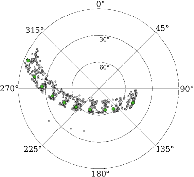
Figure 1.— Azimuthal-elevation source distribution over the sky at station hn-vlba during 11-h long experiment bt085f. Source $1609+190$ is highlighted by a big green filled circle. Other sources are displayed as small outlined grey circles.

Unfortunately, the archive magnetic tape with correlator output from two experiments, bt085d and bt085e, had deteriorated to the extent that it could not be read, and the data were completely lost. Therefore, we were able to re-analyze only 16 out of 18 experiments for a total of 857 sources.

3. Data analysis

The data were correlated at the Socorro hardware VLBA correlator. The correlator computed the spectrum of cross correlation and autocorrelation functions with a frequency resolution of 0.5 MHz and accumulation intervals 1.96608 s long.

3.1. Post-correlation analysis

The procedure of further analysis is described in complete detail in Petrov et al. (2011). Here only a brief outline is given. First, the fringe amplitudes were corrected for the signal distortion in the sampler and then were calibrated according to measurements of system temperature and elevation-dependent gain. Phase of the phase-calibration signal was subtracted from the fringe phases. Then the group delay, phase delay rate, group delay rate, and fringe phase were determined for the RR polarization (i.e. right circular polarization (RCP) at a reference station correlated against the RCP at a remote station of a baseline) for all observations, using the wide-band fringe fitting procedure. These estimates maximize the sum of the cross-correlation spectrum coherently averaged over all accumulation periods of a scan and over all frequency channels in all intermediate frequencies (IFs). After the first run of fringe fitting, an observation at each baseline with the reference station (kp-vlba) with the strongest signal to noise ratio (SNR) were used to compute the station-based complex bandpass corrections of the RR cross-correlation spectrum. The initial bandpass is the cross spectrum coherently averaged over time divided by the average of each IF. If the bandpass characteristics of each IF were constant over an experiment, then applying the bandpass, i.e. dividing the cross-spectrum by the bandpass, would make the cross-spectrum averaged over time completely flat, which reduces the coherence loss. This procedure was repeated for 12 sources with the strongest SNR at each baseline, and the results were averaged.

Next, we computed the polarization complex bandpass. This was done for each baseline with a reference station in two steps. First, we selected a scan with the highest SNR, applied the initial RR complex bandpass and computed group delay $\tau_{g}$, group delay rate $\dot{\tau_{g}}$, phase delay $\tau_{p}$, and phase delay rate $\dot{\tau_{p}}$ at the reference frequency using RR data. Then we applied the RR complex bandpass to the LL data $C^{LL}_{kj}$ at the $k$th accumulation period at the $j$th spectral channel and rotated its phase using parameters of the fringe fitting to the RR data:

$$C^{LL}_{kj}\times e^{-i\,(\,\omega_{0}(\tau_{p}\;+\;\dot{\tau}_{p}(t_{k}-t_{0}))\;\;-\;\;2(\psi_{1}-\psi_{2})\;\;+\;\;(\omega_{j}-\omega_{0})\tau_{g}\,)}.$$ (1)

where $\omega_{0}$ is the reference frequency, $t_{0}$ is the fringe reference time, $\omega_{j}$ is the frequency of the $j$th spectral channel, and $t_{k}$ is time of the $k$th accumulation period. We also subtracted the doubled difference of parallactic angles $(\psi_{1}-\psi_{2})$ at the reference and remote stations of a baseline. The latter correction accounts for the fact that the phase rotation due to a change of the receiver orientation with respect to some reference parallactic angle is opposite for the RCP and LCP (left circular polarization) signal. The residual amplitudes were normalized at each IF by its average over all spectral channels. We approximated the normalized residual complex spectrum with the Legendre polynomial of the 5th degree. These polynomials define the so-called initial polarization bandpass. It was found that using polynomials of higher degree did not provide further improvements.

Next, we processed 12 observations with the highest SNR at each baseline with the reference station. We applied the sampler correction, phase calibration to the RR data, computed parameters of the fringe fitting to the RR data, applied the sampler correction, phase calibration, performed the phase rotation according to expression 1 to the LL data of the same observation, and divided the residual spectrum by the initial complex polarization bandpass. The phase and the logarithm of the amplitude of the residual LL spectrum are used as the right-hand side of the observation equations that approximate the residual complex polarization bandpass with Legendre polynomials of the 5th degree polynomial for each IF and station, except the reference station. This system of linear equations is solved using least squares (LSQ). The product of these estimates with the initial polarization bandpass forms the final complex polarization bandpass.

The procedure of computing group delays was repeated with the complex polarization bandpass applied to all the data and using the Stokes parameter $I$, i.e. the linear combination of RR and LL cross-spectrum $C_{RR}$ and $C_{LL}$: $1/2(C_{RR}+C_{LL}/P_{b})/B_{RR}$, where $B_{RR}$ is the complex bandpass for the RR data, and $P_{b}$ is the polarization bandpass.

If the electronics of every IF were stable during the experiment and observed sources are completely unpolarized, the SNR of the coherent sum over time and frequency of the Stokes parameter $I$ would have been a factor of $\sqrt{2}$ times the SNR when only RR or LL polarization data are used. Analysis of the SNR ratios of Stokes parameter $I$ data to the SNR of RR data showed that achieved SNR was on average 96% of its theoretical value.

This part of the analysis is done with $\cal PIMA$  software.

3.2. Astrometric analysis

The results of fringe fitting the linear combination of RR and LL data were exported to the VTD/post-solve VLBI analysis software for interactive processing of the group delays with SNR high enough to ensure the probability of false detection is less than 0.001. This SNR threshold is $5.5$ for the VIPS experiment. A detailed description of the method for evaluation of the detection threshold can be found in Petrov et al. (2011). Next, theoretical path delays were computed according to the state-of-the art parametric model as well as their partial derivatives. Small differences between group delays and theoretical path delay were estimated using a least squares adjustment to the parametric model that describes the observations. Coordinates of target sources, positions of all stations (except the reference station), parameters of the spline that models residual path delay in the neutral atmosphere in the zenith direction for all stations, and parameters of another spline that models the clock function, were solved for in LSQ solutions that used group delays of the Stokes parameter $I$. Outliers of the preliminary solution were identified and temporarily barred from the solution.

The most common reason for an observation to be marked as an outlier is a misidentification of the main maximum of the two-dimensional Fourier-transform of the cross-spectrum. The procedure of fringe fitting was repeated for observations marked as outliers. Using parameters of the VLBI model adjusted in the preliminary LSQ solution, we can predict group delay for outliers with accuracy better than 1 ns. Then we re-run the fringe fitting procedure for observations marked as outliers in the narrow search window $\pm 1$ ns within the predicted value of the group delay. New estimates of group delays with probabilities of false detection less than 0.1, which corresponds to the SNR $>4.6$ for the case of a narrow fringe search window, are used in the next step of the preliminary analysis procedure. The observations marked as outliers in the preliminary solution and detected in the narrow window at the second round of the fringe fitting procedure, were tried again. If the new estimate of the residual was within 3.5 standard deviations, the observation was restored and used in further analysis. Parameter estimation and elimination of remaining outliers were then repeated. Finally, the additive weight corrections were computed in such a way that these corrections, added in quadrature to the a priori weights computed on the basis of group delay uncertainties evaluated by the fringe fitting procedure, will make the ratio of the weighted sum of residuals to their mathematical expectation close to unity.

In total, $310\,653$ estimates of group delays out of $347\,803$ scheduled were used in the solution. The number of observations of 95% of the target sources was in the range 200–440, with the median number 377. Each source was detected, except 1058+245 (catalog ). Detailed analysis showed that there are two objects in the field of view near 0748+582 (catalog ). The companion 0748+58A (catalog ) is $72^{\prime\prime}.8354$ apart.

The result of the preliminary solution provided the clean dataset of group delays with updated weights. We used this dataset and all dual-band S and X data acquired under absolute astrometry and space geodesy programs from April 1980 through April 2011, in total 8.2 million observations, to obtain final parameter estimation. Thus, the VIPS experiments were analyzed by exactly the same way as all other VLBI experiments. The estimated parameters were right ascensions and declination of all sources, coordinates and velocities of all stations, coefficients of the B-spline expansion of non-linear motion for 18 stations, coefficients of harmonic site position variations of 48 stations at four frequencies: annual, semi-annual, diurnal, semi-diurnal, and axis offsets for 69 stations. Estimated variables also included the Earth orientation parameters for each observing session and parameters of clock function and residual atmosphere path delays in the zenith direction modeled with the linear B-spline with interval 60 minutes. All parameters were adjusted in a single LSQ run.

The system of LSQ equations has an incomplete rank and defines a family of solutions. In order to pick a specific element from this family, we applied the no-net rotation constraints on the positions of 212 sources designated as “defining” in the ICRF catalogue (Ma et al. 1998) that required the positions of these sources in the new catalogue to have no rotation with respect to the position in the ICRF catalogue. No-net rotation and no-net translation constraints on site positions and linear velocities were also applied. The specific choice of identifying constraints was made to preserve the continuity of the new catalogue with other VLBI solutions made during last 15 years.

The global solution sets the orientation of the array with respect to an ensemble of $\sim\!\!\!5000$ extragalactic remote radio sources. The orientation is defined by the continuous series of Earth orientation parameters and parameters of the empirical model of site position variations over 30 years evaluated together with source coordinates. Over 400 common sources observed in the VIPS provided a firm connection between the new catalogue and the old catalogue of compact sources.

3.3. Accounting for the ionosphere contribution

Since the observations were made at a relatively low frequency of 5 GHz, one may expect that the dominant source of errors will be the mismodeled ionosphere contribution. The superior way to alleviate the frequency-dependent contribution of the ionosphere to group delays is to record simultaneously at two widely separated frequencies, i.e. 2.3 GHz (S-band) and 8.6 GHz (X-band) and to use ionosphere-free linear combinations of these observables in the data analysis. The residual delay due to high order terms that are not eliminated in the combination of observables is at a level of several ps (Hawarey et al. 2005), which is negligible.

In the absence of simultaneous dual-band observations, we computed the ionospheric path delays from the TEC maps derived from the analysis of Global Positioning System (GPS) observations using the analysis center CODE (Schaer 1998). Using GPS-derived TEC maps for data reduction of astronomic observations, first suggested by Ros (2000), has become a traditional approach for data processing. However, we should be aware that these path delays are an approximation of the ionospheric contribution and they cannot account completely for the contribution of the ionosphere. First, the TEC model has rather a coarse resolution: 5°in spatial coordinates and $2^{h}$ in time. Therefore, ionospheric fluctuations on time scales less than several hours cannot be represented by this model. Second, the model itself is not precise, since the number of GPS stations that were used for deriving the model (179 in January 2006) is relatively small and their distribution around the globe is far from homogeneous.

The availability of dual-band observations at the VLBA network during the period of time overlapping with the VIPS campaign prompted us to use this dataset for characterizing the residual errors of ionospheric path delays from GPS TEC maps. Since the ionospheric electron density varies by more than one order magnitude during a Solar activity cycle, we restricted our analysis to 15 twenty-four hour experiments under geodetic program RDV (Petrov et al. 2009) and VCS6 (Petrov et al. 2008) over the period of time from June 2005 through March 2007. In total, over $130,000$ dual-band observations were used for comparison. For each observation, we computed the contribution of the ionosphere to group delay at 4.8 GHz from both X-band and S-band VLBI group delay observables and from GPS TEC maps. The technique of further analysis is described in details in Petrov et al. (2011). Here we briefly outline it.

For each baseline and each experiment, we computed two statistics: $RV\!$, which stands for root mean square (rms) of the differences in the ionospheric group delay between VLBI and GPS measurements, and $RG=\sqrt{\mbox{rms}_{g1}^{2}+\mbox{rms}_{g2}^{2}}$, where $\mbox{rms}_{gi}$ is the rms of the GPS path delay at the $i$ th station of a baseline during a session. As we found previously, these statistics are highly correlated. For each baseline we computed a linear regression between them: $RV_{b}=F_{b}+S_{b}\cdot RG_{b}$. The coefficients $F_{b}$ and $S_{b}$ depend on the baseline. Using this regression, we can predict for a given baseline the rms of the residual contribution of group delay computed from GPS TEC maps.

3.4. Error analysis

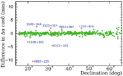
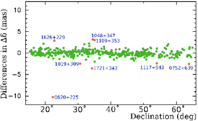
Figure 2.— Differences in positions of common sources derived from analysis of VIPS observations at C-band against positions derived from analysis of dual-band X/S observations.

One half of the sources scheduled for VIPS has been observed as part of the VLBA Calibrator Survey (Beasley et al. 2002, Fomalont et al. 2003, Petrov et al. 2005, 2006, Kovalev et al. 2007, Petrov et al. 2008) and RDV program (Petrov et al. 2009) aiming to determination of source positions in the absolute astrometry mode with the highest accuracy. These observations were made simultaneously at X and S-bands. We can compare the positions of common sources from single-band VIPS observations with dual-band observations and, considering the positions from dual-band observations as the ground truth, derive the error model.

We scrutinized the list of 430 common sources and discarded from the list 54 objects with position uncertainties from X/S observations exceeding 1 mas. We are aware that the positions of 386 common sources from the VIPS catalogue were made from both VIPS observations and all others observations. We cannot exclude all common sources from the VIPS solution, since in that case the matrix of observations will be altered and properties of such a solution would be significantly different from the properties of the VIPS catalogue. To circumvent this problem, we sorted the list of remaining 386 sources in ascending order of right ascensions and split it into two subsets of 193 sources each, even and odd. Then we ran two special solutions: solution A that had 193 sources from the even subset excluded in all experiments, except VIPS, and solution B that had 193 sources from the odd subset excluded in all experiments, except VIPS. The solution setup, except the differences in the source list, was identical to that used for deriving the VIPS catalogue. In all solutions we estimated positions of 5317 sources. We obtained positions of common sources from these two solutions derived only from the C-band VIPS observations and then combined them to form a catalogue of 386 objects.

A comparison of these two catalogues is shown in Figure 2. We present the source position differences in right ascensions and declinations as a function of source declinations. We see that for a majority of sources, the differences look like a random noise and do not exhibit any systematic pattern. There are several outliers, the most notable is 0820+225 (catalog ) (See Figure 3 and Table 1). Analysis of images of 0820+225 (catalog ), 1108+201 (catalog ), 1323+321 (catalog ), and eight others revealed a common pattern: all are sources with multiple distinctive components, and the relative strength of components varies between bands. Therefore, source positions are related to different parts of the source. A similar phenomenon was noticed during analysis of differences of X/S and K-band (24 GHz) positions reported by Petrov et al. (2011). On average, 1% sources exhibit this behavior.

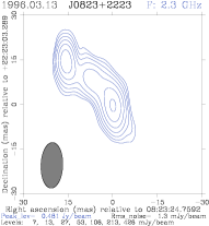
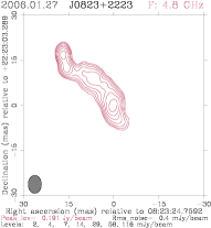
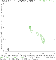
Figure 3.— Image of J0823+2223 (0820+225) in four frequency bands. The center of the image is set to the brightest component. The images at X and S bands are produced from analysis of VCS1 observations (Kovalev, private communication), the image at C-band was produced from analysis of VIPS observations, and the image at U-band was produced from analysis of observations from the MOJAVE program (Lister et al. 2009).

Table 1The table of sources with the greatest differences between VIPS and X/S positions. Quoted flux densities are the median correlated flux densities at baselines longer than 5000 km.

Dist	Err	B1950-name	J2000-name	Comment
(mas)	(mas)
14.6	0.5	0820$+$225	J0823$+$2223	Long, complex jet
5.0	0.4	1323$+$321	J1326$+$3154	CSO
3.6	0.5	1721$+$343	J1723$+$3417	Long, complex jet
3.4	0.4	1048$+$347	J1050$+$3430	Double source (core-jet)
3.4	0.4	1108$+$201	J1111$+$1955	CSO
3.1	0.4	1109$+$353	J1112$+$3503	Weak: 76 mJy at 8 GHz
3.0	0.4	1600$+$244	J1602$+$2418	CSO candidate
2.9	0.4	1626$+$229	J1628$+$2247	Long, complex jet
2.8	0.4	1019$+$309	J1022$+$3041	Long, complex jet
2.6	0.5	1117$+$543	J1120$+$5404	Weak: 38 mJy at 8 GHz
2.6	0.7	0752$+$639	J0756$+$6347	Strong core-jet
2.4	0.4	0932$+$367	J0935$+$3633	Double source (core-jet)
2.2	0.5	1221$+$464	J1223$+$4611	Weak: 67 mJy at 8 GHz
2.1	0.4	1525$+$314	J1527$+$3115	Long, complex jet

After removing the outliers, we sought for the ad hoc variance that, when added in quadrature with the formal error, makes the ratio of the weighed sum of the differences to their mathematical expectation close to unity. We found that the additional variance for right ascensions scaled by cosine of declination is 0.24 mas and the variance for declinations is 0.31 mas. The weighted root mean squares (wrms) of the differences in right ascensions scaled by cosine of declination is 0.44 mas and the wrms of the differences in declination is 0.58 mas.

We should note that our estimate of the additive variances provides an upper limit on the errors. First, de-selecting sources in trial solutions A and B weakened these solutions with respect to the solution used for deriving the VIPS catalogue and increased position errors of common sources. Second, the additive variances 0.24 and 0.31 mas are comparable with errors of the reference X/S solution. Therefore, the additive variances reflect contributions of errors of both C-band VIPS and the X/S catalogues.

4. Source position catalogue

Table 2The first 12 rows of the VIPS catalogue of source positions of 857 sources. The table columns are explained in the text. The full table is available in the electronic attachment.

									Correlated flux density (in Jy)
Flag	Source Names		J2000 Coordinates		Errors (mas)				S-band		C-band		X-band
	IVS	IAU	Right   ascension	Declination	$\Delta\alpha$	$\Delta\delta$	Corr	# Obs	Total	Unres	Total	Unres	Total	Unres
(1)	(2)	(3)	(4)	(5)	(6)	(7)	(8)	(9)	(10)	(11)	(12)	(13)	(14)	(15)
X	0552$+$398	J0555$+$3948	05 55 30.805615	$+$39 48 49.16493	0.40	0.24	-0.032	1775	3.457	2.765	6.957	4.226	4.736	2.144
C	0716$+$450	J0719$+$4459	07 19 55.511712	$+$44 59 06.84827	1.68	1.52	-0.059	98	$\cdots$	$\cdots$	0.151	¡0.02	$\cdots$	$\cdots$
C	0722$+$393	J0726$+$3912	07 26 04.737260	$+$39 12 23.32117	0.55	0.57	-0.300	302	$\cdots$	$\cdots$	0.076	0.045	$\cdots$	$\cdots$
C	0722$+$415	J0726$+$4124	07 26 22.420172	$+$41 24 43.66844	0.53	0.43	-0.217	362	$\cdots$	$\cdots$	0.106	0.090	$\cdots$	$\cdots$
C	0722$+$615	J0726$+$6125	07 26 51.681732	$+$61 25 13.68060	0.90	0.42	-0.017	336	$\cdots$	$\cdots$	0.096	0.088	$\cdots$	$\cdots$
X	0723$+$488	J0727$+$4844	07 27 03.100595	$+$48 44 10.12669	0.52	0.34	-0.004	362	0.447	0.357	0.263	0.222	0.330	0.280
X	0729$+$562	J0733$+$5605	07 33 28.615274	$+$56 05 41.73927	2.34	1.98	-0.238	86	0.099	1.269	0.113	0.022	$\cdots$	$\cdots$
C	0731$+$595	J0735$+$5925	07 35 56.300840	$+$59 25 22.11156	0.94	0.48	0.022	322	$\cdots$	$\cdots$	0.053	0.037	$\cdots$	$\cdots$
X	0733$+$300	J0736$+$2954	07 36 13.661088	$+$29 54 22.18498	0.41	0.42	-0.038	344	0.464	0.409	0.273	0.158	0.302	0.178
C	0733$+$287	J0736$+$2840	07 36 31.198545	$+$28 40 36.80515	2.05	1.97	-0.144	58	$\cdots$	$\cdots$	0.039	0.025	$\cdots$	$\cdots$
X	0733$+$261	J0736$+$2604	07 36 58.073689	$+$26 04 49.94573	0.41	0.42	-0.034	351	0.336	0.086	0.240	0.108	0.326	0.215
C	0734$+$269	J0737$+$2651	07 37 54.975269	$+$26 51 47.44790	0.54	0.60	-0.141	302	$\cdots$	$\cdots$	0.071	0.051	$\cdots$	$\cdots$

Note. — Table 2 is presented in its entirety in the electronic edition of the Astronomical Journal. A portion is shown here for guidance regarding its form and contents. Units of right ascension are hours, minutes and seconds. Units of declination are degrees, minutes and seconds.

Table 2 displays 12 out of 857 rows of the VIPS catalogue of source positions. The full table is available in the electronic attachment. Column 1 contains the source flag: “X” if the sources was previously observed at X and S-bands under absolute astrometry programs, “C” otherwise. Columns 2 and 3 contain the J2000 and B1950 IAU names; column 4, and 5 contain right ascensions and declinations. Columns 6 and 7 contain positional uncertainties in right ascension (without multiplier $\cos\delta$) and in declinations with noise added in quadrature to their formal errors. Column 8 contains correlation coefficients between right ascension and declination, column 9 contains the total number of observations used in position data analysis. Columns 10 through 15 contain the median estimates of the correlated flux density over all experiments of a given source in two ranges of baseline projection lengths: less than 900 km, and longer than 5000 km. The first estimate is close to the total correlated flux density, the second estimate is close to the correlated flux density of the unresolved component. The estimates of the median correlated flux densities are given for three bands: S-band (columns 10,11), C-band (columns 12,13), and X-band (columns 14,15). The estimate of the flux density at C-band was computed from analysis of VIPS data by Helmboldt et al. (2007), estimates at S and X band are from re-analysis of VCS and RDV observations. If there were no detections at the range of the baseline projection lengths, then $-1.000$ is put in the table cell.

The histogram of the semi-major axes of position uncertainties is given in Figure 4.

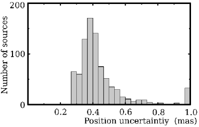
Figure 4.— The histogram of semi-major axes of inflated position uncertainties of the VIPS source position catalogue. The last bin shows uncertainties exceeding 1 mas.

5. Discussion

The astrometric accuracy of VIPS exceeded our expectations. Although absolute astrometry was not considered at all during design of the experiment, position uncertainties of target sources observed in single band VIPS experiments at 5 GHz turned out better than the position uncertainties of dedicated VCS experiments. The contribution of the residual ionosphere path delay after applying the GPS-derived TEC model was small and did not affect the positional accuracy significantly.

Several factors contributed to this success. First, the wide-band frequency setup spanned over 494 MHz was used. This is essential. If a contiguous bandwidth of 32 MHz had been recorded, as is often selected in imaging experiments, group delays would have been a factor of 22 less precise, and as a result, the source position accuracy would have been more than one order of magnitude worse. Second, each source was scheduled in 10 scans equally distributed over the hour angle of the array center (station pietown). The schedule was optimized to get good ($u,v$)-coverage with no elevation cutoff enforced. Observations at elevations as low as $3\arcdeg$ were scheduled. Good ($u,v$)-coverage also provides a good separation among variables of interest such as source coordinates, as well as among nuisance parameters such as the clock function. Frequent scheduling of low-elevation observations improves the reliability of estimates of residual atmosphere path delay in zenith parameters, since it helps to decorrelate these parameters with station positions and clock function parameters. Third, the integration time was correctly predicted, so the vast majority of sources were detected at both short and long baselines. A lack of observations at long baselines reduces the accuracy of source positions significantly. Finally, the experiments were carried out during the Solar minimum when ionosphere disturbances were exceptionally low.

Of the 14 sources with significant discrepancies between their position measured in VIPS and that derived from dual-band X/S observations (see Table 1, the majority (10/14) have complex structure in which the brightest component is a function of angular resolution and/or observing frequency. This includes three Compact Symmetric Objects which generally have more complex structure than core-jets. Of the remainder, three sources are core-jets, but quite weak ($<$ 100 mJy/beam), so it is likely that in this case the errors are less systematic and more the result of low SNR. The single remaining source, VIPS J0756+6347 (catalog ), is a strong and ordinary core-jet and the reason for the discrepancy in positions is unclear.

6. Conclusions

We have determined positions of 857 sources observed in 16 VIPS experiments. Milliarcsecond-accurate coordinates of 430 objects were determined with VLBI for the first time.

We found that during the Solar minimum the residual ionosphere contribution to the group delay after applying the reduction for path delay from GPS TEC map is small enough not to cause systematic errors exceeding 0.3 mas at frequencies as low as 5 GHz.

Our error analysis showed that for 95% of the sources the uncertainty of their positions range from 0.3 to 0.9 mas. This estimate is substantiated by comparison with a large set of 386 VIPS sources that were also observed in X/S absolute astrometry programs. The position uncertainty of the VIPS catalogue is better than the uncertainty of dedicated VLBI Calibration Surveys.

References

- Abdo et al. (2010) Abdo, A. A., Ajello, M., Antolini, E., et al. 2010, ApJ, 715, 429
- Adelman-McCarthy et al. (2006) Adelman-McCarthy, J. K., Agüros, M., A., Allam, S. S., et al. 2006, ApJS, 162, 38
- Beasley et al. (2002) Beasley, A. J., Gordon, D., Peck, A. B., et al. 2002, ApJS, 141, 13
- Fomalont et al. (2003) Fomalont, E., Petrov, L., McMillan, D. S., Gordon, D., & Ma, C. 2003, AJ, 126, 2562
- Healey et al. (2007) Healey, S. E., Romani, R. W., Taylor, G. B., et al. 2007, ApJS, 171, 61
- Helmboldt et al. (2007) Helmboldt, J. F., Taylor, G. B., Tremblay, S., et al. 2007, ApJ, 658, 203
- Hawarey et al. (2005) Hawarey, M., Hobiger, T., and Schuh, H. 2005, Geophys. Res. Lett., 32, L11304
- Kovalev et al. (2007) Kovalev, Y. Y., Petrov, L., Fomalont, E., Gordon, D. 2007, AJ, 133, 1236
- Lindegren et al. (2008) Lindegren, L., Babusiaux, C., Bailer-Jones, C., et al. 2008, in Proc. IAU Symposium, 248, 217
- Linford et al. (2011) Linford, J. D., Taylor, G. B., Romani, R. W., et al. 2011, ApJ, 726, 16
- Lister et al. (2009) Lister, M. L., Aller, H. D., Aller, M. F., et al. 2009, AJ, 137, 3718
- Ma et al. (1998) Ma, C., Arias, E. F., Eubanks, T. M., et al. 1998, AJ, 116, 516
- Marscher et al. (2006) Marscher, A. P. 2006, AIP Conf. Proc. 856: Relativistic Jets: The Common Physics of AGN, Microquasars, and Gamma-Ray Bursts, 856, 1
- Myers et al. (2003) Myers, S. T., Jackson, N. J., Browne, I. W. A., et al. 2003, MNRAS, 341, 1
- Petrov et al. (2005) Petrov, L., Kovalev, Y. Y., Fomalont, E., Gordon, D. 2005, AJ, 129, 1163
- Petrov et al. (2006) Petrov, L., Kovalev, Y. Y., Fomalont, E., Gordon, D. 2006, AJ, 131, 1872
- Petrov et al. (2008) Petrov, L., Kovalev, Y. Y., Fomalont, E., Gordon, D. 2008, AJ, 136, 580
- Petrov et al. (2009) Petrov, L., Gordon, D., Gipson, J., et al. 2009, Jour. Geod., 83, 859
- Petrov et al. (2011) Petrov, L., Kovalev, Y. Y., Fomalont, E., Gordon, D., 2011, AJ, 142, 35
- Ros (2000) Ros, E., Marcaide, J. M., Guirado, J. C., Sardón, E., & Shapiro, I. I. 2000, A&A, 356, 357
-
Schaer (1998)
Schaer, . 1998, Ph.D. thesis, Univ. Bern; accessible at
ftp://ftp.unibe.ch/aiub/papers/ionodiss.ps.gz - Taylor (2005) Taylor, G. B., Fassnacht, C. D., Sjouwerman, L. O., et al. 2005, ApJS, 159, 2007
- Taylor et al. (2007) Taylor, G. B., Healey, S. E., Helmboldt, J. F., et al. 2007, ApJ, 671, 1355
- York et al. (2000) York, D., Adelman, J., Anderson, J. E., et al. 2000, AJ, 120, 1579