Long-range steady state density profiles induced by localized drive

Abstract

We show that the presence of a localized drive in an otherwise diffusive system results in steady-state density and current profiles that decay algebraically to their global average value, away from the drive in two or higher dimensions. An analogy to an electrostatic problem is established, whereby the density profile induced by a driving bond maps onto the electrostatic potential due to an electric dipole located along the bond. The dipole strength is proportional to the drive, and is determined self-consistently by solving the electrostatic problem. The profile resulting from a localized configuration of more than one driving bond can be straightforwardly determined by the superposition principle of electrostatics. This picture is shown to hold even in the presence of exclusion interaction between particles.

The effect of a local perturbation on the steady state density profile of systems of interacting particles has been studied in a wide variety of contexts. When a system under thermal equilibrium conditions is perturbed by a localized external potential, the equilibrium density is changed only locally under generic conditions. This is a result of the fact that as long as the system is not at a critical point, it is characterized by a finite correlation length. This is not necessarily the case in driven systems where detailed balance is not satisfied ZIA . Algebraically decaying correlations in the steady state profiles have been found in a number of boundary driven models such as the Asymmetric Simple Exclusion Process (ASEP) BLYTH , interface growth models KM and transport models in one and higher dimensions LIVI ; DHAR ; SPOHN .

A natural question is what happens when the drive is localized not on the boundaries but in the bulk. In a recently studied model of a one-dimensional Symmetric Simple Exclusion Process (SSEP) it was shown that the presence of a single driving bond (battery) in the bulk does not generate any algebraic density profile in the steady state BDL . The density profile was found to be flat away from the battery, albeit with a discontinuity at the location of the battery.

In the present Letter we consider the effect of driving bonds localized in a finite region in an infinitely large many body system. We demonstrate that under rather generic conditions a localized drive in an otherwise equilibrium system in dimensions higher than one, results in a steady state density profile with an algebraically decaying tail. This is done by first studying the case of non-interacting particles diffusing on a d-dimensional lattice with a directional drive along a single bond (battery). We then generalize the results to arbitrary localized configurations of driving bonds, and to the case of particles with exclusion interaction.

In the case of non-interacting particles with a single driving bond, we show that the density profile can be mapped onto the electrostatic potential generated by an electric dipole located at the driving bond, whose strength can be calculated self-consistently. Thus, for example, in $d=2$ dimensions, the density profile decays as $1/r$ at distance $r$ away from the driving bond, in all directions except the one perpendicular to the drive, where it decays as $1/r^{2}$. More interestingly, other localized configurations of driving bonds result in different power-law profiles. In this case the density profile can be determined by a linear superposition of the profiles generated by each driving bond. For example, when the electric dipoles corresponding to two driving bonds form a quadrupole, the density profile generically decays as $1/r^{2}$ while in some specific directions it decays as $1/r^{4}$, at large distances. The correspondence to the electrostatic problem still holds when local exclusion is switched on. The only difference is in the dipole strength which, unlike the noninteracting case, can not be determined self-consistently. In the interacting case, our results thus generalize the one dimensional situation studied in BDL and show that for $d\geq 2$, the density profile decays algebraically away from the battery.

We start with the simple case of non-interacting particles diffusing in a medium with a single driving bond. As an illustration we consider explicitly the $d=2$ case. Generalization to arbitrary dimensions is straightforward. We consider a two-dimensional square lattice of $L\times L$ sites with periodic boundary conditions. There are $N=\rho V$ noninteracting particles where $V=L^{2}$ is the number of sites and $\rho$ is the global average density of particles. Each particle performs an independent random walk in continuous time. A particle at site $\vec{r}\equiv(m,n)\neq(0,0)$ can hop to any of the neighboring sites with rate $1$. We introduce a localized drive by setting the hopping rate across the bond $(0,0)\to(1,0)$ to be $(1-\epsilon)$ with $\epsilon\leq 1$ (see Fig.1a). In the absence of the localized drive ($\epsilon=0$), detailed balance holds and the system reaches a steady state with a flat density profile with density $\rho$ at each site. When the localized drive $\epsilon$ is switched on, it manifestly violates the detailed balance and induces a global modification of the steady state density profile.

Figure 1: (a) Bond-configuration with a single driving bond $(0,0)\rightarrow(1,0)$ and hopping rate $e=(1-\epsilon)$. Everywhere else the rate is $1$. The $\oplus$ and $\ominus$ symbols denote the sign of the electric charge. The symbol $\odot$ represents the magnetic flux coming out of the plane, and $\otimes$ represents the flux going in. (b) A configuration of closed loop of driving bonds generating no electric charges. The magnetic flux through the central plaquette is four times larger than that of the other four neighboring plaquettes.

Let $\phi(m,n,t)$ denote the average density of particles at site $(m,n)$ at time $t$. Its time evolution can be easily written down by counting the incoming and outgoing moves from each site. For sites $(m,n)\neq\{(0,0),(1,0)\}$, it is easy to see $\phi(m,n,t)$ satisfies the standard diffusion equation, $\partial_{t}\phi(m,n,t)=\nabla^{2}\phi(m,n,t)$, where $\nabla^{2}$ is the discrete Laplacian: $\nabla^{2}\phi(m,n)=\phi(m+1,n)+\phi(m-1,n)+\phi(m,n+1)+\phi(m,n-1)-4\phi(m,n)$. The evolution equations are slightly different for the two special sites $(0,0)$ and $(1,0)$ connecting the driving bond: $\partial_{t}\phi(0,0,t)=\nabla^{2}\phi(0,0,t)+\epsilon\phi(0,0,t)$ and $\partial_{t}\phi(1,0,t)=\nabla^{2}\phi(1,0,t)-\epsilon\phi(0,0,t)$. It is useful to write these evolution equations in a combined form by introducing Kronecker delta symbols. For brevity, let us also denote ${\vec{r}}=(m,n)$, ${\vec{0}}=(0,0)$ and ${\vec{e}_{1}}=(1,0)$. In the long time limit the system approaches a time independent steady state $\phi(\vec{r})$ satisfying

$$\nabla^{2}\phi(\vec{r})=-\epsilon\phi(\vec{0})\left[\delta_{\vec{r},\vec{0}}-\delta_{\vec{r},\vec{e}_{1}}\right]$$ (1)

for all $\vec{r}$. Here $\delta_{\vec{r},\vec{r}^{\prime}}$ is the Kronecker delta function. It is instructive to first note the formal resemblance of (1) with the Poisson equation (lattice version) of the $2$-d electrostatic problem. One identifies $\phi(\vec{r})$ as the electrostatic potential and the right hand side (rhs) of (1) is identified with two point charges of equal strength but of opposite signs sitting respectively at the two ends of the driving bond. Thus we have effectively a dipole sitting on the weak bond. However, unlike in standard electrostatics the charge strength $\epsilon\phi(\vec{0})$ has to be determined self-consistently.

We consider the thermodynamic limit $L\to\infty$, $N\to\infty$ with density per site $\rho=N/V$ fixed. The exact solution of (1) at any $\vec{r}$ can be expressed in terms of the lattice Green’s function $G(\vec{r},{\vec{r}_{0}})$ which is the Coulomb potential due to a single point charge of unit strength at $\vec{r}_{0}$, that satisfies $\nabla^{2}G=-\delta_{\vec{r},{\vec{r}_{0}}}$. Using the superposition principle one obtains the solution

$$\phi(\vec{r})=\rho+\epsilon\phi(\vec{0})\left[G(\vec{r},\vec{0})-G(\vec{r},\vec{e}_{1})\right].$$ (2)

The constant $\phi(\vec{0})$ can be determined self-consistently by substituting $\vec{r}=\vec{0}$ in (2). This gives, $\phi(\vec{0})=\rho/[1-\epsilon(G(\vec{0},\vec{0})-G(\vec{0},\vec{e}_{1})]$. Then by evaluating the lattice Green’s function for an infinite square SPITZER , one finds $\phi(\vec{0})=\rho/[1-\epsilon/4]$.

To determine the large distance behavior of the solution, one can use the continuum approximation under which the Green’s function behaves as $G(\vec{r},{\vec{r}_{0}})\approx-\frac{1}{2\pi}\ln|\vec{r}-{\vec{r}_{0}}|$, for large $|\vec{r}-{\vec{r}_{0}}|$. Substituting in (2), one finds that the density in (2) decays for large $r$ algebraically as

$$\phi(\vec{r})=\rho-\frac{\epsilon\phi(\vec{0})}{2\pi}\frac{{\vec{e}_{1}}\cdot{\vec{r}}}{r^{2}}+\mathcal{O}(\frac{1}{r^{2}}).$$ (3)

This density profile also leads to a nontrivial current profile. The average particle current density, away from the drive, is ${\vec{j}}(\vec{r})=-\nabla\phi(\vec{r})$ and it decays for large $r$ as

$${\vec{j}}(\vec{r})=\frac{\epsilon\phi(\vec{0})}{2\pi}\,\frac{1}{r^{2}}\,\left[{\vec{e}_{1}}-\frac{2({\vec{e}_{1}}\cdot{\vec{r}}){\vec{r}}}{r^{2}}\right]+\mathcal{O}(\frac{1}{r^{3}}).$$ (4)

In the electrostatic analogue, ${\vec{j}}(\vec{r})$ is precisely the electric field generated by the dipole.

Due to the superposition principle, the above analysis can be readily generalized to the case of arbitrary localized configuration of the driving bonds. For example, consider a case of two driving bonds with rates $(1-\epsilon)$ each, one from $(0,0)$ to $(1,0)$ and the other from $(0,0)$ to $(-1,0)$, while the rates across the rest of the bonds in the lattice are fixed to be $1$ in both ways:

$$\cdots(-2,0)\,\overset{1}{\underset{1}{\leftrightarrows}}\,(-1,0)\,\overset{1-\epsilon}{\underset{1}{\leftrightarrows}}\,(0,0)\,\overset{1-\epsilon}{\underset{1}{\rightleftarrows}}\,(1,0)\,\overset{1}{\underset{1}{\rightleftarrows}}\,(2,0)\cdots$$

It is again easy to see that the steady state density $\phi(\vec{r})$ now satisfies

$$\nabla^{2}\phi(\vec{r})=-\epsilon\phi(\vec{0})\left[2\delta_{\vec{r},\vec{0}}-\delta_{\vec{r},\vec{e}_{1}}-\delta_{\vec{r},-\vec{e}_{1}}\right].$$ (5)

In the electrostatic analogue, the rhs of (5) corresponds to two oppositely oriented adjacent dipoles on the $x$ axis, constituting a quadrupole charge configuration $(-++-)$ in the continuum limit. Using the two-dimensional Coulomb potential and the superposition principle, it is easy to see that the density profile at large distance $r$ now decays as

$$\phi(\vec{r})=\rho-\frac{\epsilon\phi(\vec{0})}{2\pi}\left[\frac{1}{r^{2}}-2\left(\frac{{\vec{e}_{1}}\cdot{\vec{r}}}{r^{2}}\right)^{2}\right]+\mathcal{O}(\frac{1}{r^{4}}),$$ (6)

with $\phi(\vec{0})=\rho/(1-\epsilon/2)$. Consequently, the particle current density (or equivalently the electric field of the quadruple) ${\vec{j}}(\vec{r})$ decays as $r^{-3}$ for large $r$.

In the case of an arbitrary configuration of $n$ driving bonds, one uses the superposition principle to express the steady state profile in terms of the dipole strengths of the $n$ dipoles. Using the exact expression for the Green’s function on square lattice SPITZER a set of linear equations determining these strengths are obtained, which can be readily solved.

The existence of biased bonds does not necessarily imply a breakdown of detailed balance. Localized configurations of biased bonds may preserve detailed balance with respect to a localized potential $V(\vec{r})$. For example, consider the case where all incoming links to the site $(0,0)$ are with rates $(1-\epsilon)$ each and the rates across the rest of the links in the lattice are fixed to be $1$. It is easy to verify that the rates satisfy detailed balance with respect to the localized potential $V(\vec{r})=-\ln(1-\epsilon)\,\delta_{\vec{r},\vec{0}}$. Consequently, the steady state density has the Gibbs-Boltzmann form $\phi(\vec{r})\propto\exp[-V(\vec{r})]$ leading to a flat density profile everywhere except at the origin.

It is interesting to note that in $d=2$ dimension, the analogy to an electrostatic problem can be extended to introduce a magnetic field as well. In a general two-dimensional setting let $e_{ij}$ denote the hopping rate from site $i$ to its nearest neighbor site $j$. This link creates a pair of oppositely directed flux lines centered on the two plaquettes that share this link. The flux is perpendicular to the plaquettes, with, say, the flux to the left of the link points up (see Fig.1a). The magnitude of the field generated by the $(ij)$ bond is given by $H=\ln\left(\frac{e_{ij}}{e_{ji}}\right)$. The total flux through each plaquette is given by the sum of the fluxes generated by each of its links. A necessary and sufficient condition for detailed balance to hold is the vanishing of the total magnetic field, as defined above, on all plaquettes. This is a direct consequence of the Kolmogorov criterion KLMGRV ; DAVID . In that case, the density profile outside the driven region is flat resulting in a vanishing electric field, as follows from the Boltzmann measure. However when the magnetic field is non-zero, the steady state is a nonequilibrium one, and the density profile created by the driving bonds typically decays algebraically. On the other hand, bond configurations which result in vanishing electric field and non-vanishing magnetic field has a flat density profile. An example of such configuration is given in Fig.1b.

Another interesting density profile pattern emerges when one applies a global bias, say in the $x$-direction. Consider again noninteracting particles in $d=2$, where a particle from any site $(m,n)$ hops to a neighboring site with rate $1$ in the north, west and south directions, while with rate $(1+\mu)$ to the eastern neighbor. Thus, $\mu\geq 0$ denotes the global bias. In addition, there is the driving bond from $(0,0)\to(1,0)$ where the hopping rate is set to be $(1+\mu-\epsilon)$ with $0\leq\epsilon\leq 1$. Proceeding as before, in the steady state, $\phi(\vec{r})$ is found to satisfy

$$-\mu\,\left[\phi(\vec{r})-\phi(\vec{r}-\vec{e}_{1})\right]+\nabla^{2}\phi(\vec{r})=-\epsilon\phi(\vec{0})\left[\delta_{\vec{r},\vec{0}}-\delta_{\vec{r},\vec{e}_{1}}\right]$$ (7)

where $\vec{r}-\vec{e}_{1}\equiv(m-1,n)$ and $\nabla^{2}$ is the discrete Laplacian as before. The solution can be expressed as

$$\phi(\vec{r})=\rho+\epsilon\phi(\vec{0})\left[g(\vec{r},\vec{0})-g(\vec{r},\vec{e}_{1})\right]$$ (8)

where the Green’s function $g(\vec{r},\vec{r}_{0})$ satisfies

$$-\mu\,\left[g(\vec{r},\vec{r}_{0})-g(\vec{r}-\vec{e}_{1},\vec{r}_{0})\right]+\nabla^{2}g(\vec{r})=-\delta_{\vec{r},\vec{r}_{0}}.$$ (9)

The solution can be obtained using Fourier transformation. Setting $(X,Y)\equiv\vec{r}-\vec{r}_{0}$, one finds that for large $X$, $Y$

$$g(X,Y) \simeq \frac{1}{\sqrt{4\pi\mu\,X}}\,e^{-\mu Y^{2}/{4X}},\,\quad X>0$$ (10)

$$\simeq \frac{e^{\mu X}}{\sqrt{4\pi\mu\,|X|}}\,e^{-\mu Y^{2}/{4|X|}},\,\quad X<0.$$ (11)

These results have a nice interpretation as the solution of a diffusion equation where $X$ plays the role of ‘time’ and $Y$ the distance traveled from the origin. It can be directly seen from (9) which, for large $(X,Y)$, can be approximated by its continuum version: $-\mu\partial_{X}g+\partial_{X}^{2}g+\partial_{Y}^{2}g=0$. For large $X>0$, neglecting the term $\partial_{X}^{2}$, one indeed obtains an analogue of diffusion equation, $\mu\partial_{X}g=\partial_{Y}^{2}g$ with $\mu$ playing the role of friction coefficient and $X>0$ being the ‘time’ variable and hence one obtains the standard diffusive propagator in (10) for $X>0$. In contrast, for negative $X$, one can no longer interpret directly in terms of the diffusion equation in which the ‘time’ is always a positive variable. However, upon making a change of variable $X\to-X^{\prime}$ and substituting $g(X,Y)=e^{-\mu X^{\prime}}h(X^{\prime},Y)$ one gets $\mu\partial_{X^{\prime}}h=\partial_{X^{\prime}}^{2}h+\partial_{Y}^{2}h$. This leads to the result (11) for $X<0$. Substituting this result for the Green’s function in (8) one obtains a density profile $\phi(x,y)$ that is highly anisotropic. For example, for $y=0$ and as $x\to+\infty$, the density decays algebraically to $\rho$ as $x^{-3/2}$ while in the direction opposite to the bias $x\to-\infty$, the density decays exponentially. In the $y$ direction, for fixed $x$, the density falls off rapidly as $\sim\exp\left[-\mu y^{2}/{4|x|}\right]$.

The $2$-d results obtained above for noninteracting particles, with or without global bias, can be easily generalized to arbitrary dimensions. Indeed, the solution in (2) holds for arbitrary dimensions $d$, except that the Green’s function $G(\vec{r},\vec{r}_{0})$ depends on $d$. In the continuum limit, the Couloumb potential $G(\vec{r},\vec{r}_{0})$ behaves, for large $|\vec{r}-\vec{r}_{0}|$, as $|\vec{r}-\vec{r}_{0}|^{-(d-2)}$ for $d>2$, as $-\frac{1}{2\pi}\ln|\vec{r}-\vec{r}_{0}|$ for $d=2$ and as $-\frac{1}{2}|\vec{r}-\vec{r}_{0}|$ for $d=1$. Hence, the dipole potential and consequently the density profile $\phi(\vec{r})$ decays as $r^{-(d-1)}$ for large $r$ in $d\geq 2$. In $d=1$, the dipole potential has a discontinuity at $x=0$, thus giving rise to a discontinuous density profile: $\phi(x)=\rho-(\epsilon/2)\,\phi(0)\,{\rm sgn}(x)$, in full accordance with BDL . The results for quadrupoles and higher multi-poles can similarly be generalized to arbitrary dimensions. The analogy to a magnetic field discussed earlier is, however, restricted only to two dimensions.

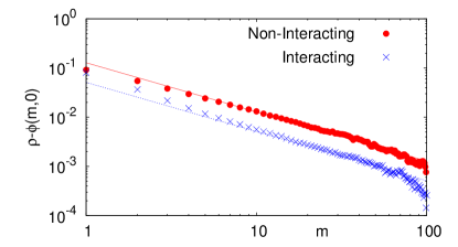
Figure 2: The algebraic decay of the density profile away from the driving bond in the positive $x$ direction.

We now show that most of the results derived above for noninteracting particles in presence of a localized drive carry through when the hard core interaction between the particles is switched on. We consider a symmetric exclusion process on a $2$-d square lattice where each site can hold at most one particle. Our results are easily generalizable to arbitrary dimensions. From any occupied site $(m,n)$ the particle attempts to hop to any of its neighboring sites with rate $1$ and actually hops there provided the target site is empty. As in the noninteracting case, we introduce the localized drive across the bond $(0,0)\to(1,0)$ where the attempted hopping rate is $(1-\epsilon)$ with $\epsilon\leq 1$. It is useful to first associate an occupation variable $\tau(\vec{r},t)$ with every site $\vec{r}$: $\tau(\vec{r},t)=1$ if the site $\vec{r}$ is occupied at time $t$ and is zero if it is empty at $t$. Clearly, the average density is $\phi(\vec{r},t)=\langle\tau(\vec{r},t)\rangle$. It is again easy to write down the time evolution equation of $\phi(\vec{r},t)$ by counting the incoming and outgoing rates from each site. In this case the equation analogous to (1) is

$$\nabla^{2}\phi(\vec{r})=-\epsilon\langle\tau(\vec{0})(1-\tau(\vec{e}_{1})\rangle\,\left[\delta_{\vec{r},\vec{0}}-\delta_{\vec{r},\vec{e}_{1}}\right],$$ (12)

where $\phi(\vec{0})$ in (1) is replaced by $C=\langle\tau(\vec{0})(1-\tau(\vec{e}_{1})\rangle$. While, unlike in the noninteracting case, we can not determine this prefactor self-consistently, the electrostatic analogy to a dipole (albeit with an unknown strength $\epsilon C$) still holds. Thus, at long distances, one still obtains a long-ranged algebraic decay of the density profile

$$\phi(\vec{r})=\rho-\frac{\epsilon C}{2\pi}\frac{{\vec{e}_{1}}\cdot{\vec{r}}}{r^{2}}+\mathcal{O}(\frac{1}{r^{2}}).$$ (13)

Consequently, the particle current density (equivalently the electric field due to the dipole) ${\vec{j}}(\vec{r})$, decays at large distances as in the noninteracting case (4), up to an overall multiplicative constant. In a similar way, one can also arrange the driving bonds so as to generate a quadrupole or multi-pole configurations of charges giving rise to an algebraic decay of the density profile with varying exponents depending on the charge configurations.

A numerical evidence of the profiles in (3) and (13) is shown in Fig.2 where the difference of density from $\rho$ is plotted against the distance from the driving bond in the positive $x$ direction. The simulation is performed on a $200\times 200$ lattice with $\epsilon=1$ and initial uniform density $\rho=0.6$. The straight lines denote the theoretical results in (3) and (13) with the value of $\phi(0)$ calculated using $\rho$ and $\epsilon$, and $C=\langle\tau(0)(1-\tau(\vec{e}_{1}))\rangle=0.3209$ determined independently from the Monte Carlo simulation.

In summary, we have demonstrated that in diffusive systems, both with and without inter particle exclusion interaction, localized drive can give rise to algebraically decaying density profiles at large distances. The problem of determining the density profile is mapped onto an electrostatic problem where each driving bond is represented by an electric dipole whose strength is determined self-consistently by the electric potential generated on the driving bond. The density profile of the driven system is then given by the electrostatic potential created by the charge distribution. An analogous quantity to the magnetic field is also identified in two dimensions.

We thank M. R. Evans and O. Hirschberg for their constructive comments on an earlier draft of this paper. The support of the Israel Science Foundation (ISF) is gratefully acknowledged. This work was carried out while S.N.M. was a Weston Visiting Professor at the Weizmann Institute of Science.

References

- (1) B. Schmittmann and R.K.P. Zia, Statistical Mechanics of Driven Diffusive Systems edited by C. Domb, and J.L. Lebowitz, Academic Press, (1995).
- (2) R.A. Blythe, M.R. Evans, J. Phys. A-Math. Theo. 40, R333 (2007).
- (3) D. Kandel and D. Mukamel, Europhys. Lett. 20, 325 (1992).
- (4) S. Lepri, R. Livi, A. Politi, Phys. Rep. 377, 1 (2003).
- (5) A. Dhar, Advances in Physics 57, 457 (2008).
- (6) H. Spohn, J. Phys. A-Math. Gen. 16, 4275 (1983).
- (7) T. Bodineau, B. Derrida, and J.L. Lebowitz, J. Stat. Phys. 140, 648 (2010).
- (8) F. Spitzer, Principles of Random walk, Springer, page 148 (2001).
- (9) F.P. Kelly, Reversible and Stochastic Networks, Wiley, page 22 (1979).
- (10) D. Mukamel in Soft and Fragile Matter, Nonequilibrium Dynamics, Metastability and Flow edited by M. E. Cates, and M. R. Evans, Institute of Physics Publishing, Bristol, (2000) p. 237, arXiv:cond-mat/0003424.