Stability of magnetic nanoparticles inside ferromagnetic nanotubes

Abstract

During the last years great attention has been given to the encapsulation of magnetic nanoparticles. In this work we investigated the stability of small magnetic particles inside magnetic nanotubes. Multisegmented nanotubes were tested in order to optimize the stability of the particle inside the nanotubes. Our results evidenced that multisegmented nanotubes are more efficient to entrap the particles at temperatures up to hundreds of kelvins.

Interest in magnetic nanostructures has increased dramatically over the past decade, mainly due to the great progress in experimental techniques and recent technological developments which allow access to interesting length scales. In particular, understanding the behaviour of solids in confined geometries at the nanoscale is an important area of basic research which has a strong potential for applications LHH+09 ; Parkin09 ; FLH+06 . Within this area, carbon nanotubes have stimulated intensive experimental and theoretical research since their discovery in 1991 Iijima91 . One of the topics that have been considered is the encapsulation of nanoparticles for different purposes. In particular, paramagnetic nanoneedles have been encapsulated KYG+05 , preventing them from agglomeration when a magnetic field is not present and allowing control of the needles’ movement. The carbon encapsulation of ferromagnetic nanoparticles has also been reported BLH07 ; RBS+10 ; KHK+08 , opening an interesting field of research. In particular, encapsulation of Ni BZH+02 , Co BTX+02 , Fe FCW+07 ; MMP+10 ; SC08 and Ga LHX+09 inside multi-walled carbon nanotubes has been reported and magnetically characterized using vibrating sample magnetometers and superconducting quantum interference devices. Also, the stability and magnetic properties of Fe encapsulated in silicon nanotubes has been explored, finding a high local magnetic moment per Fe atom, and a transition between from antiferromagnetic to a ferromagnetic coupling is obtained by increasing the length of the nanotube WZM+07 .

Besides this intense study on the encapsulation of magnetic nanoparticles, few attention has been given to the encapsulation of nanoparticles inside magnetic nanotubesEBJ+08 . Magnetic nanotubes have been prepared since 2005 KNR+05 by K. Nielsch and his group. Also barcode-type nanostructures have been prepared. In particular, Lee et al. LSN+05 reported the synthesis of multisegmented metallic nanotubes with a bimetallic stacking configuration along the tube axis, showing a different magnetic behavior as compared with continuous ones.

Following these ideas, the focus of this work is the stability of a magnetic nanoparticle inside a ferromagnetic nanotube. Using Monte Carlo simulations we investigate different nanotubes, looking for the magnetic configuration that increases the stability of an encapsulated magnetic nanoparticle. To investigate the behaviour of a nanoparticle inside a magnetic nanotube we start by calculating the magnetic fieldEAA+08 due to the nanotube over the points of a three-dimensional grid $\left(\{\vec{r}_{i}\}\right)$. This step is accomplished by adding up the contributions to the overall magnetic field coming from each atom that constitutes the nanotube (the magnetic dipolar field). Then we simulate the random walk of a magnetic nanoparticle over the field landscape generated by the nanotube. This is done by means of a Monte Carlo simulation in which the nanoparticle starts at the center of the nanotube and is allowed to move over the grid and to rotate its magnetic moment under the influence of the tube’s field.

The starting point is the definition of the crystalline structure of the tube, i. e., we define the Bravais lattice, the lattice constant ($a_{\mbox{\tiny 0}}$) and the magnetic moment per atom ($\mu_{\mbox{\tiny 0}}$). The simulations shown in this paper consider BCC iron as the constituting species, which gives us $a_{\mbox{\tiny 0}}=0.2866\ \mbox{nm}$ and $\mu_{\mbox{\tiny 0}}=2.22\ \mu_{\mbox{\tiny B}}$. An important point is the definition of the three-dimensional grid over which the field will be calculated and the energy of the particle will be tested. For our calculations we have chosen a grid that is commensurate with the lattice structure and that considers the available computational facilities. According to these requirements, we have used as the grid step ($\Delta$), the nearest multiple to $5\ \mbox{nm}$ of $a_{\mbox{\tiny 0}}$, hence, $\Delta=17\ a_{\mbox{\tiny 0}}=4.8722\ \mbox{nm}$. However, we have also tried smaller and larger $\Delta$ ($\Delta=8\ a_{\mbox{\tiny 0}}$ and $52\ a_{\mbox{\tiny 0}}$, respectively) and no fundamental differences were observed compared with the results obtained using $\Delta=17\ a_{\mbox{\tiny 0}}.$

The next step is to define the tube’s overall dimensions. The tube’s height, which is also commensurate with $a_{\mbox{\tiny 0}}$, was chosen to be $L_{\mbox{\scriptsize tube}}=205\ \Delta=998.8\ \mbox{nm}$. The radial dimensions were set to $R_{\mbox{\scriptsize e}}=50\ \mbox{nm}$ (external radius) and $R_{\mbox{\scriptsize i}}=40\ \mbox{nm}$ (internal radius). We investigate the behaviour of the particle using multilayer nanotubes composed of magnetic and non-magnetic segments, as illustrated in Fig. 1. The length of the non-magnetic segment, the spacer, has also been varied (see Fig. 2) to obtain the desired field landscape, but similar results are obtained if one uses a non optimal choice.

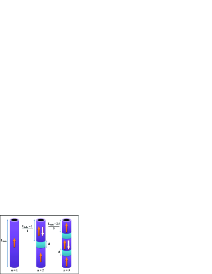
Figure 1: (Color online) Illustration of the different tube geometries that we have tested, depicting the magnetic and non-magnetic regions. The white arrows represent what we call an antiparallel segments.

Even a nanotube with such dimensions would contain more than 240 million atoms, rendering extremely expensive any attempt of direct calculations, regardless of the computational power available. To circumvent this technical issue, we first calculate the field generated over the grid points $\left(\{\vec{r}_{i}\}\right)$ by all the magnetic moments inside a ring ($\rho_{\mbox{\tiny 0}}$) of height $\Delta$ which is magnetized along its axis and located at the centre of the grid. We used the usual expression (Eq. 1), for the field of a collection of magnetic dipoles and stored our results for each point of the grid in a file. The latter was used as a building block to construct the desired tube.

$$\vec{B}_{0}\left(\vec{r}_{i}\right)=\sum_{a\ \in\ \rho_{\mbox{\tiny 0}}}\frac{3\vec{\mu}_{a}\cdot\left(\vec{r}_{i}-\vec{r}_{a}\right)}{|\vec{r}_{i}-\vec{r}_{a}|^{5}}\left(\vec{r}_{i}-\vec{r}_{a}\right)\\ -\frac{\vec{\mu}_{a}}{|\vec{r}_{i}-\vec{r}_{a}|^{3}}+\frac{8\pi}{3}\vec{\mu}_{a}\delta\left(\vec{r}_{i}-\vec{r}_{a}\right),$$ (1)

where the indices $a$ and $i$ run over all the atoms belonging to the ring $\rho_{\mbox{\tiny 0}}$ and all the sites belonging to the grid, respectively.

Finally, by summing the contributions coming from different rings ($\rho_{n}$) centered at different positions ($\vec{r}_{n}=n\Delta\hat{z}$) with different weights ($w_{n}$), we are able to construct multi-segmented tubes LSL+09 with as many parallel or antiparallel aligned segments as we want (just by weighting their contribution by $\pm 1$) and separated by non-magnetic materials (by weighting their contribution by 0) as follows.

$$\vec{B}_{\mbox{\scriptsize tube}}\left(\vec{r}_{i}\right)=\sum_{n=-N}^{+N}w_{n}\vec{B}_{0}\left(\vec{r}_{i}-\vec{r}_{n}\right),$$ (2)

where $N=\left(L_{\mbox{\tiny tube}}-\Delta\right)/2\Delta$. The result of such calculation is depicted in Fig. 2, which shows the field along the tube’s axis obtained from Eq. 2 for one or two segments while keeping the full length of the tube fixed at $998.8\mbox{ nm}$, as illustrated in Fig. 1. In this figure we can observe that for thinner spacers the antiparallel alignment provides a higher magnetic field in the centre of the tube compared to the parallel alignment.

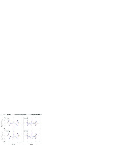
Figure 2: (Color online) The magnetic field along the tube’s axis obtained from Eq. 2 for one or two segments while keeping the length fixed.

Above we have defined the set of grid points occupied by the tube itself and the magnetic field $\vec{B}\left(\{\vec{r}_{i}\}\right)$ that it creates. So now we are in position to investigate the stability of a nanoparticle inside the tube. We start by putting the particle, characterized by its position $\left(\vec{r}\ \in\{\vec{r}_{i}\}\right)$ and magnetic moment vector $\left(\vec{\mu}\right)$, in the center of the tube and let it move and rotate under the Hamiltonian

$$\mathcal{H}=-\vec{\mu}\cdot\vec{B}\left(\vec{r}\right)\ .$$

The magnitude of the moment $\vec{\mu}$ is chosen to represent a Co nanoparticle with diameter $\Delta$ whose magnetic moment initially points in a random direction. At each Monte Carlo step, a movement and a new orientation for the magnetic moment are proposed simultaneously. The movement consists in walking one step on the grid along one of the six possible directions $\left(+\hat{x},-\hat{x},+\hat{y},-\hat{y},+\hat{z},-\hat{z}\right)$. The new orientation is sampled randomly from a sphere with radius $|\vec{\mu}|$.

The energy difference caused by the new position and orientation is calculated and the Monte Carlo step is accepted (or not) by means of the standard Metropolis algorithm at a given temperature $T$ BH02 . All the simulations shown on this paper were done using a total of $10^{7}$ Monte Carlo steps. Then we repeat this procedure $2\times 10^{3}$ times in order to get the average walk of the particle on the magnetic field landscape of the tube.

We have performed the above-mentioned procedure for different tube geometries, magnetic configurations and temperatures. We have chosen the geometry in which the non-magnetic spacer is $d=51a_{\mbox{\tiny 0}}$ thick because thinner spacers would allow long-range magnetic interactions (such as RKKY) to play an undesired role by strengthening the coupling between different segments. Our results are depicted in Fig. 3, which shows a measure of the average z coordinate (along the tube’s axis) of the particles as a function of the number of Monte Carlo steps (mcs). The graphs are shown in terms of $\xi=\sqrt{\langle z^{2}\rangle}/(L_{\mbox{\scriptsize tube}}/2)$. $\xi=0$ denotes that particle is at the center of the tube, $\xi\approx 0.34$ represents one of the interfaces between the spacer and the magnetic section in the three-segment nanotube, the tips of the tube are denoted by $\xi=1$, and a particle leaving the tube is denoted by $\xi>1$.

Figure 3 shows that at $T=10\mbox{ K}$ all the compound tubes are able to confine the particle while the simple tube is not. At $T=300\mbox{ K}$ none of the tubes were capable of keeping the particle trapped, although the tube with two antiparallel aligned segments was the one that mostly delayed the leaving. However, it is at $T=100\mbox{ K}$ that interesting phenomena take place: the parallel alignment of segments seems to be less effective in trapping the particle, since only the field landscape created by antiparallel aligned segments is capable of restraining the particle’s movement.

Figure 3: (Color online) Evolution of $\xi$ as a function of the number of Monte Carlo steps (mcs) for several tube geometries (one, two or three segments), different magnetic configurations (parallel or antiparallel alignment) and several temperatures ($T=10,\ 100,\ 300\mbox{ K}$). $\xi=1$ represents the tips of the tube.

We also investigate the effect of the size of the nanoparticle by increasing its diameter from $\Delta$ to $2\Delta$. Our results for $T=300$ K are presented in Fig. 4, showing that larger sizes contribute to stabilize the particle inside the tube.

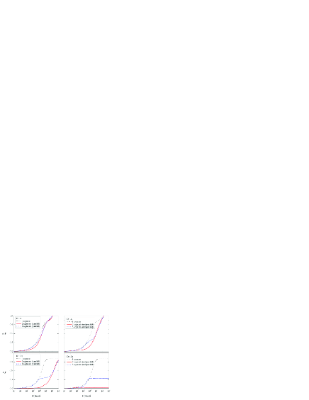
Figure 4: (Color online) Evolution of $\xi$ as a function of the number of Monte Carlo steps (mcs) for particles with diameter $\Delta$ (top) and $2\Delta$ (bottom).

From our results we can conclude that the use of multilayer geometries can help to stabilize magnetic nanoparticles inside ferromagnetic nanotubes. In spite there is still no experimental realization of these proposal, it might be possible to synthetized magnetic nanoparticles inside nanotubes by coating a multi-segmented nanotube with an oxide layer on the inner wall, using Atomic Layer Deposition (ALD). Subsequently, using electrodeposition, the nano-channel can be filled up to the middle of the pore channel with the non-magnetic segment. At the end of the electrochemical deposition a short segment of magnetic material can be deposited. Similar techniques have been used to produce multilayered core/shell nanowires by Chong et al CGM+10 and multi-segmented nanotubes by electrochemical depositionLSN+05 . Before starting the experiment, the non-magnetic metallic segment is selective etched and the oxide layer should be also selectively removed. During the removal of the oxide layer on the nanotube inner wall, and using a very strong magnetic field in the perpendicular direction to the nanotube axis, it is possible to trap and mechanically detach the magnetic particles from the template. By removing the perpendicular magnetic field the time until the particle exit the tube can be measured. Alternative it is possible to make the magnetic segments of a material with a Curie temperature around 100 ⁰C and inject the magnetic particle with a polymeric meld at a higher temperature into the channel. After cool down the polymeric meld, it will solidify. The polymeric filling can be removed using an organic solution and a strong magnetic field perpendicular to the nanotube’s diameter. In this way, these procedures can guide the design of experiments which can test our results.

Looking at what happened at $T=100\mbox{ K}$, it seems possible to use the alignment between the segments as a switch to open or close the particle’s exit. If one constructs a tube with two segments, one made of a soft and the other of a hard magnetic material, one could in principle use an external magnetic field to switch the direction of magnetization of the softer segment, thus changing from antiparallel to parallel alignment and facilitating the departure of the walking particle.

If one wants to increase the temperature where the free/trapped behaviour occurs when using parallel/antiparallel alignment (in our case, $T=100\mbox{ K}$ for particles with diameter $\Delta$) one can simply use walking particles with larger magnetic moments to increase the magnitude of the Zeeman energy ($E_{\mbox{\tiny Zeeman}}=-\vec{\mu}\cdot\vec{B}$) with respect to the thermal energy ($k_{\mbox{\tiny B}}T$).

In Chile we acknowledge support from FONDECYT under grants 1080300, 11070010, and 3090047, the Millennium Science Nucleus “Basic and Applied Magnetism” P06-022-F, and Financiamiento Basal para Centros Científicos y Tecnológicos de Excelencia. In Brazil we ackowledge PROSUL and CNPq. In Germany we acknowledge support from the German Research Council (DFG) in the framework of the Sonderforschungsbereich SFB668 Magnetismus vom Einzelatom zur Nanostruktur and by the Excellence Cluster “Nanosprintronics” .

References

- (1) J. H. Lee, S. N. Holmes, B. Hong, P. E. Roy, M. D. Mascaro, T. J. Hayward, D. Anderson, K. Cooper, G. A. C. Jones, M. E. Vickers, C. A. Ross, and C. H. W. Barnes, Appl. Phys. Lett. 95, 172505 (2009).
- (2) Stuart S. P. Parkin, Scientific American Magazine 300, 76-81 (2009).
- (3) Hong Jin Fan, Woo Lee, Robert Hauschild, Marin Alexe, Gwenael Le Rhun, Roland Scholz, Armin Dadgar, Kornelius Nielsch, Heinz Kalt, Alois Krost, Margit Zacharias and Ulrich Gosele, Small 2, 561-568 (2006).
- (4) Sumio Iijima, Nature 354, 56-58 (1991).
- (5) Guzeliya Korneva, Haihui Ye, Yury Gogotsi, Derek Halverson, Gary Friedman, Jean-Claude Bradley, and Konstantin G. Kornev, Nano Lett. 5, 879-884 (2005).
- (6) M. Bystrzejewski, H. Lange, and A. Huczko, Fullerenes, Nanotubes and Carbon Nanostructures 15, 167-180 (2007).
- (7) Daniel Bretas Roa, Ingrid David Barcelos, Abner de Siervo, Kleber Roberto Pirota, Rodrigo Gricel Lacerda, and Rogerio Magalhaes-Paniago, Appl. Phys. Lett. 96, 253114 (2010).
- (8) Konstantin G. Kornev, Derek Haverlson, Guzeliya Korneva, Yury Gogotsi, and Gary Friedman, Appl. Phys. Lett. 92, 233117 (2008).
- (9) Jianchun Bao, Quanfa Zhou, Jianming Hong, and Zheng Xu, Appl. Phys. Lett. 81, 4592 (2002).
- (10) J. Bao, C. Tie, Z. Xu, Z. Suo, Q. Zhou, and J. Hong, Advanced Materials 14, 1483-1486 (2002).
- (11) Takeshi Fujita, Mingwei Chen, Xiaomin Wang, Bingshe Xu, Koji Inoke, and Kazuo Yamamoto, J. Appl. Phys. 101, 014323 (2007).
- (12) Francisco Munoz, Jose Mejía-López, Tomas Pérez-Acle, and Aldo H. Romero, ACS Nano 4, 2883-2891 (2010).
- (13) C. X. Shi, and H. T. Cong, J. Appl. Phys. 104, 034307 (2008).
- (14) K. Li, H. Y. He, B. Xu, and B. C. Pan, J. Appl. Phys. 105, 054308 (2009).
- (15) Jianguang Wang, Jijun Zhao, Li Ma, Guanghou Wang, and R. Bruce King, Nanotechnology 18, 235705 (2007).
- (16) J. Escrig, J. Bachmann, J. Jing, M. Daub, D. Altbir, and K. Nielsch, Phys. Rev. B 77, 214421 (2008).
- (17) K. Nielsch, F. J. Castaño, C. A. Ross, and R. Krishnan, J. Appl. Phys. 98, 034318 (2005) .
- (18) Lee W, Scholz R, Nielsch K and Gosele U, Angew. Chem. Int. Edn 44, 6050 (2005).
- (19) J. Escrig, S. Allende, D. Altbir, and M. Bahiana, Appl. Phys. Lett. 93, 023101 (2008).
- (20) B. Leighton, O. J. Suarez, P. Landeros, and J. Escrig, Nanotechnology 20, 385703 (2009).
- (21) K. Binder, and D. W. Heerman, Monte Carlo Simulation in Statistical Physics (Springer, New York, 2002).
- (22) Y. T. Chong, D. Gorlitz, S. Martens, M. Y. E. Yau, S. Allende, J. Bachmann. K. Nielsch, Advanced Materials 22, 2435 (2010).