HST/ACS Observations of Europa’s Atmospheric UV Emission at Eastern Elongation

Abstract

We report results of a Hubble Space Telescope (HST) campaign with the Advanced Camera for Surveys to observe Europa at eastern elongation, i.e. Europa’s leading side, on 2008 June 29. With five consecutive HST orbits, we constrain Europa’s atmospheric O I 1304 Å  and O I 1356 Å  emissions using the prism PR130L. The total emissions of both oxygen multiplets range between 132 $\pm$ 14 and 226 $\pm$ 14 Rayleigh. An additional systematic error with values on the same order as the statistical errors may be due to uncertainties in modelling the reflected light from Europa’s surface. The total emission also shows a clear dependence of Europa’s position with respect to Jupiter’s magnetospheric plasma sheet. We derive a lower limit for the O₂ column density of 6 $\times$ 10¹⁸ m^-2. Previous observations of Europa’s atmosphere with STIS in 1999 of Europa’s trailing side show an enigmatic surplus of radiation on the anti-Jovian side within the disk of Europa. With emission from a radially symmetric atmosphere as a reference, we searched for an anti-Jovian vs sub-Jovian asymmetry with respect to the central meridian on the leading side and found none. Likewise, we searched for departures from a radially symmetric atmospheric emission and found an emission surplus centered around 90${{}^{\circ}}\;$west longitude, for which plausible mechanisms exist. Previous work about the possibility of plumes on Europa due to tidally-driven shear heating found longitudes with strongest local strain rates which might be consistent with the longitudes of maximum UV emissions. Alternatively, asymmetries in Europa’s UV emission can also be caused by inhomogeneous surface properties, inhomogeneous solar illuminations, and/or by Europa’s complex plasma interaction with Jupiter’s magnetosphere.

1 Introduction

Jupiter’s satellite Europa is an outstandingly interesting body in our solar system as several lines of evidence point to a subsurface water ocean under its icy crust. Europa is a differentiated body with an outer layer of H₂O with a thickness of $\sim$100 km Anderson et al. (2007); Hussmann et al. (2002). Its surface is relatively young with an average age of $\sim$60 Myr and it is much less heavily cratered than its two neighboring satellites Ganymede and Callisto (e.g., Greeley et al., 2004). Evidence for Europa’s subsurface ocean comes from observations of geological structures (e.g., Pappalardo et al., 1999; Greeley et al., 2004). Europa’s surface is rich in various features, such as ridges, chaotic regions, and cycloids possibly due to flexing of its icy crust under tidal forces (e.g., Pappalardo et al., 1999; Nimmo & Gaidos, 2002). These features are naturally explained by a subsurface ocean of liquid water, but it cannot be ruled out that they are alternatively due to processes in warm, soft ice with only localized or partial melting Pappalardo et al. (1999). A strong and fully independent argument for a subsurface ocean comes from observations of induced magnetic fields Khurana et al. (1998); Neubauer (1998); Kivelson et al. (2000); Zimmer et al. (2000); Schilling et al. (2007); Saur et al. (2010) which require a subsurface layer with a sufficiently large electrical conductivity. Within Europa’s geological and geophysical context, only saline liquid water is considered a viable candidate to achieve the required conductivity.

Europa also possesses a thin oxygen atmosphere discovered with the Goddard High-Resolution Spectrograph (GHRS) of the Hubble Space Telescope by Hall et al. (1995). Observed fluxes of 11.1 $\pm$ 1.7 $\times$ 10^-5 photons cm^-2 s^-1 and 7.1 $\pm$ 1.3 $\times$ 10^-5 photons cm^-2 s^-1 (at the Telescope), corresponding to a brightness of 69 $\pm$ 13 and 37 $\pm$ 15 Rayleigh, for the two oxygen multiplets O I 1356 Å   and O I 1304 Å  , respectively, implied a very thin molecular oxygen atmosphere with a surface pressure of about 10^-11 bar Hall et al. (1995, 1998). The radiation is excited predominately by electron impact dissociation of molecular oxygen. The previous observations were taken on 1994 June 02 at western elongation, i.e. on Europa’s trailing hemisphere. Subsequent observations on 1996 July 21 with GHRS on the leading hemisphere rendered fluxes of 8.6 $\pm$ 1.2 $\times$ 10^-5 photons cm^-2 s^-1 (54.7 $\pm$ 7.6 R) for O I 1304 and 12.9 $\pm$ 1.3 $\times$ 10^-5 photons cm^-2 s^-1 (82.1 $\pm$ 8.3 R) for O I 1356. Observations on 1996 July 30 confirmed the oxygen atmosphere on the trailing hemisphere with 12.6 $\pm$ 1.3 $\times$ 10^-5 (80.2 $\pm$ 8.3 R) for O I 1304 and 14.2 $\pm$ 1.5 $\times$ 10^-5 (90.4 $\pm$9.5 R) for O I 1356 Hall et al. (1998). The joint fluxes of both oxygen multiplets were thus 18.2 $\times$ 10^-5 photons cm^-2 s^-1 (106 R) on the trailing side in 1994, 26.8 $\times$ 10^-5 photons cm^-2 s^-1 (170 R) also on the trailing side in 1996, and 21.5 $\times$ 10^-5 photons cm^-2 s^-1 (137 R) on the leading side in 1996. Based on these observations, Hall et al. (1998) estimated O₂ column densities in the range of 2.4 to 14 $\times$ 10¹⁸ m^-2. Comprehensive reviews on Europa’s atmosphere can be found in McGrath et al. (2004, 2009).

Europa’s atmosphere is considered to be primarily generated through surface sputtering by magnetospheric ions Johnson et al. (1982); Pospieszalska & Johnson (1989); Shi et al. (1995); Shematovich et al. (2005). Dominant loss processes are atmospheric sputtering and ionization. The balance of production and loss rates, which both also depend on the electromagnetic field environment establishes the average atmospheric content. Estimations of this balance leads to a O₂ column density of $\sim$5 $\times$ 10¹⁸ m^-2 and a neutral O₂ loss rate of $\sim$50 kg s^-1 Saur et al. (1998). The neutral loss, including H₂ from thermal escape, generates a neutral torus along the orbit of Europa discovered by Mauk et al. (2003) and Lagg et al. (2003).

Europa is embedded in the Jovian magnetosphere whose plasma constantly streams past Europa and its atmosphere. The interaction of the magnetospheric plasma with Europa’s atmosphere is primarily responsible for the generation of an ionosphere on Europa Kliore et al. (1997). This interaction in addition to induction in a possible sub-surface ocean creates magnetic field perturbations Kivelson et al. (1997); Saur et al. (1998); Schilling et al. (2008) and generates Alfvén wings Neubauer (1999); Saur (2004), which lead to auroral footprints of Europa in Jupiter’s upper atmosphere Clarke et al. (2002); Grodent et al. (2006). Europa’s plasma interaction modifies not only the electron density but also the electron temperature in Europa’s atmosphere. Both the electron density and temperature control the O I1304 Å  and O I 1356 Å  emission rates. Europa’s plasma interaction has been studied by Saur et al. (1998); Liu et al. (2001); Schilling et al. (2007, 2008), where the latter two models self-consistently include induction in Europa’s possible subsurface ocean.

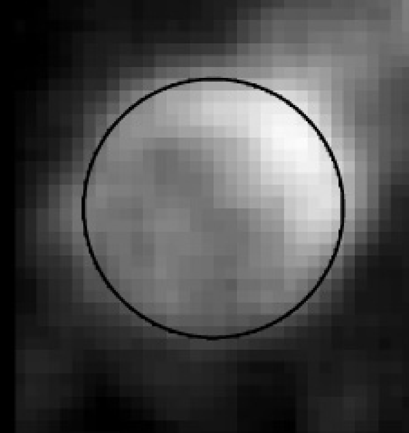
Figure 1: Europa’s O I 1356 emission at the trailing hemisphere. Image is generated from the superposition of all STIS observations on 1999 October 5 (after McGrath et al., 2004). Celestial North is up and Jupiter to the left.

After the initial spectral observation of Europa’s atmosphere by Hall et al. (1995, 1998), the first spatially resolved observations of Europa’s atmospheric emission were performed with the Space Telescope Imaging Spectrograph (STIS) in 1999 October 5 during five consecutive HST orbits McGrath et al. (2004, 2009). A superposition of all exposures is shown in Figure 1. The emission displays a clear asymmetry with respect to the sub-Jovian/anti-Jovian side. On the anti-Jovian side within the disk of Europa occurs a significant enhancement of the emission. Even though Figure 1 suggests time-stationarity of the emission, the location of the maximum of the emission moves from Europa’s northern hemisphere to its southern hemisphere, but stays predominantly on the anti-Jovian side McGrath et al. (2009). This emission is puzzling as it occurs within the disk of Europa, while for a radially symmetric atmosphere combined with a radially symmetric plasma interaction, the emission would be largest near the limb just outside of Europa’s disk. Cassidy et al. (2007) investigate such a stationary surplus of the oxygen emission and show that a non-uniform distribution of reactive species in Europa’s porous regolith can result in a non-uniform O₂ atmosphere consistent with Figure 1.

In this work we investigate HST/ACS observations of Europa’s UV emission taken on 2008 June 6 when Europa was at eastern elongation to further constrain Europa’s atmospheric content and to investigate if there are also enigmatic inhomogeneities in Europa’s UV emission on the leading hemisphere. In section 2 we present our observations at eastern elongation and describe how they were analyzed. In section 3 we present the results of our analysis and discuss their implications. Finally, in section 4 we summarize our results and point to unresolved issues.

2 Observations and Analysis

During HST program 11186, five consecutive orbits of observations with ACS/SBC prism PR130L on 2008 June 29 were taken (see Table 1). Europa was at eastern elongation, i.e. the leading side of Europa was visible from Earth. Each orbit was subdivided into four distinct exposures of $\sim$10 min. During the time of the observations Europa also crossed the current sheet of Jupiter’s magnetosphere. Europa’s positions with respect to the current sheet are indicated in Table 1.

Due to the unavailability of STIS during the time of our observations, we used the prism PR130L Bohlin et al. (2000); Larson (2006) to separate reflected solar photons from the surface of Europa and the oxygen multiplets O I 1356 Å   and O I 1304 Å   from Europa’s atmosphere. The prism covers nominally the wavelength range larger than 1216 Å   to $\sim$2000 Å   and thus suppresses Ly $\alpha$. Unfortunately, the wavelength range larger than 2000 Å  is less strongly suppressed than anticipated leading to a significant ’red leak’ (e.g. Feldman et al., 2011). The sensitivity and dispersion properties have been recalibrated on-orbit by Larson (2006). The dispersion, i.e. $\Delta\lambda$ per pixel, is a highly non-linear function of wavelength. The wavelength $\lambda$ as a function of trace distance $\Delta x$ on the detector can be written in the form

$$\lambda(\Delta x)=a_{1}+a_{2}\;(\Delta x-a_{0})^{-1}+a_{3}\;(\Delta x-a_{0})^{-2}+a_{4}\;(\Delta x-a_{0})^{-3}+a_{5}\;(\Delta x-a_{0})^{-4}$$ (1)

with the coefficients $a_{0}$ to $a_{5}$ depending on the object positions $x_{ref},y_{ref}$ in the direct image, i.e.. without prism Bohlin et al. (2000); Larson (2006). The spectral trace is additionally shifted in the y-direction on the detector as a function of wavelength as detailed in Bohlin et al. (2000) and Larson (2006).

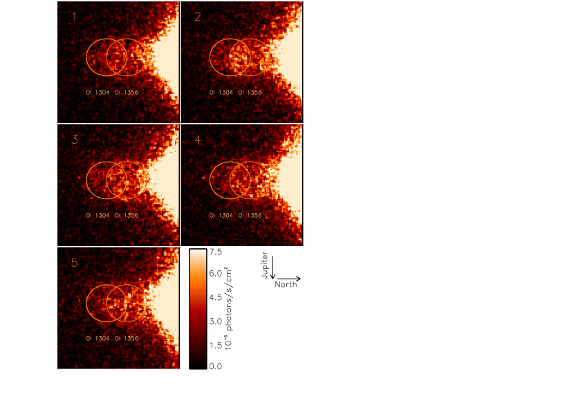
Figure 2: Five orbits of HST/ACS/SBC observations on 2008-06-29 (see Table 1). South is to the left and Jupiter is down in each image.

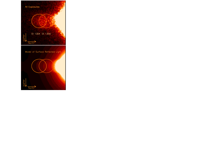
Figure 4: Sum of all exposures (top) and modelled reflected solar light from disk of Europa (bottom). The same color code is applied as in Figure 2. North is to the right and Jupiter is down in each image. The color scale is identical to the color scale of Figure 2.

In Figure 2 we display the sum of the four exposures in each orbit separately. A superposition of all exposures is shown in the top panel of Figure 4. In each image, celestial north is toward the right and defines the x-direction considered in the present study. The top of the images is towards the anti-Jovian side of Europa and is labeled y-direction. The dispersion of the prism is in the x-direction, i.e. longer wavelengths lie further to the right in each image. In each image in Figure 2 and 4, the two ellipses show the expected locations of Europa’s disk for the O I 1304 Å  and O I 1356 Å   emissions observed with the PR130L prism. Unfortunately, both images overlap. The overlap is even somewhat larger than indicated in the overlapping ellipses as the radiation from Europa’s atmosphere off the disk additionally contributes to the radiation. Therefore we analyze the sum of the O I 1304 Å  and O I 1356 Å   emission in this paper and investigate possible asymmetries of the joint emission in the y-direction only, i.e. the sub-Jovian/anti-Jovian direction, as this direction is not affected by the overlap.

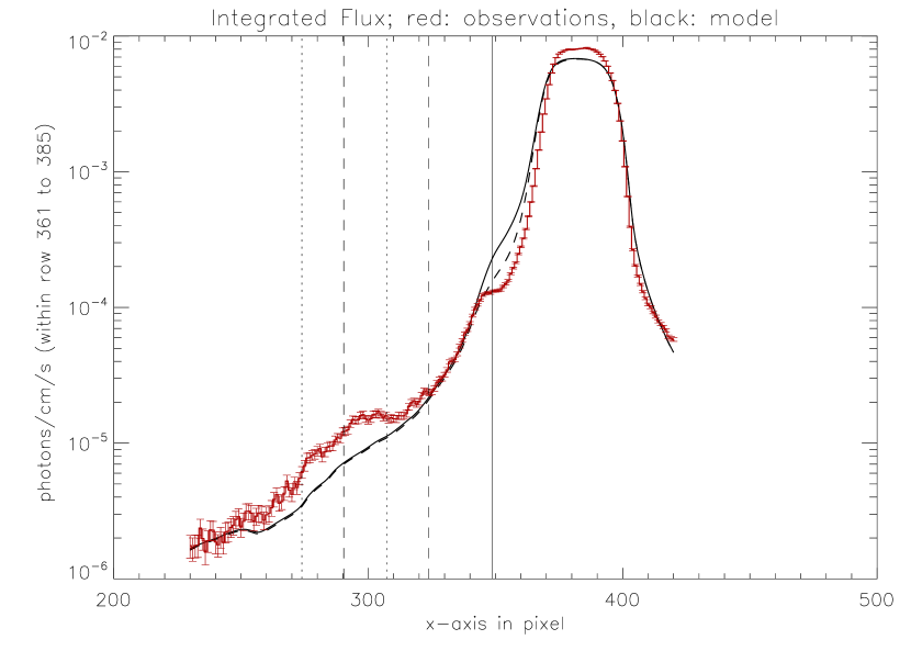
Figure 5: Observed fluxes (red) along trace (x-axis) summed along y-axis calculated with a superposition of all exposures. Modelled fluxes of solar light reflected from Europa’s surface is shown as black solid line. Reflected light calculated with an alternative model is displayed as black dashed line (further explanations in text). Vertical dotted lines show area of O1304 image and vertical dashed lines displays area of O I 1356 image.

The sunlight reflected by Europa’s surface significantly contributes to the measured fluxes. In particular, emission longward of $\sim$2000 Å   is not fully filtered out and leads to the triangle shaped emission on the right hand side of the image displayed in Figure 2. This long wavelength ’red leak’ exceeds the fluxes of the O I images by roughly two orders of magnitude much further to the right of the O I images as displayed in Figure 5.

In order to account for the contribution of the reflected sunlight to the O I images, we model its photon flux $F_{S}$ as a function of position $(x,y)$ on the detector. The reflected and dispersed solar light can be calculated as

$$F_{s}(x,y)=\int_{\mbox{solar spect}}d\lambda\;p(\lambda)t(\lambda)a(\lambda)D[x-(\Delta x(\lambda)+x_{E}),y-(y_{d}(\Delta x(\lambda))+y_{E})]$$ (2)

with the dispersion $d\lambda/d(\Delta x)$ Larson (2006) and $\Delta x(\lambda)$ being the trace distance of the dispersed photon flux in x-direction as a function of wavelength $\lambda$ compared to the location of the undispersed flux without prism. The location of the spectral trace is also shifted in the y-direction by $y_{d}(\Delta x)$ Larson (2006). The coordinates $x_{E}$, and $y_{E}$ refer to the center of Europa’s disk without dispersion. $D[x(\lambda),y(\lambda)]$ represents the disk of Europa with $D[x,y]=1$ within the disk, and $D[x,y]=0$ outside of the disk. Since we used a prism, $D$ is a function of wavelength $\lambda$. The solar photon flux $p(\lambda)$ is given by Woods et al. (1996) and displayed in Figure 3, $t(\lambda)$ is the throughput, and $a(\lambda)$ Europa’s albedo. The throughput for $\lambda<2000$ Å  is provided by Larson (2006) and constrained for $\lambda>2000$ Å  based on observations of 16 CygB as detailed in Appendix A.1. The flux $F_{s}(x,y)$ is additionally convolved with a point spread function as described in Appendix A.2.

Since no direct image of Europa was taken during the HST campaign 11186, the location of the direct image has to be reconstructed from the dispersed images. For this purpose the strong red leak is very useful. The long wavelengths reflected solar light generates in the obtained observations an easily discernible region of maximum flux corresponding to the size of Europa when plotted with a linear color scale, owing to the very low dispersion of the prism at red leak wavelengths. For this long wavelength image of Europa, we determine its coordinates and then use expression (2) to subsequently determine $x_{E}$ and $y_{E}$. The latter step is possible despite the uncertainties in the throughput for long wavelengths since the dispersion is very large at long wavelengths, e.g. $\sim 250$ Å  pxl^-1 at 4000 Å. Therefore uncertainties in the slope of the throughput at long wavelengths have very small effects on the position of the dispersed long wavelength image of Europa.

Europa’s albedo as a function of wavelength is only partially constrained by previous observations. Hall et al. (1998) derive a disk averaged albedo of 0.015 $\pm$ 0.004 on the leading side and similar albedo values on the trailing side at $\lambda=1335$ Å  . Based on an analysis of STIS observations of Europa’s trailing side in 1999 (ID 8224, PI M. McGrath), the albedo stays remarkably flat in the FUV between 1400 and 1700 Å  at values near 0.016. The constancy of the albedo values in this wavelength range (not shown here) is derived similarly to the analysis of STIS observations of Ganymede (ID 7939, PI W. Moos, Feldman et al. (2000)). Hendrix et al. (1998) find that the albedo on the leading side at central meridian of 120^∘ W increases approximately linearly from $\sim$0.2 to $\sim$0.65 within $\lambda=2200$ Å  to $\lambda=3200$ Å. Noll et al. (1995) and Hendrix et al. (1998) find a lower albedo on the trailing side which changes from $\sim$0.08 to $\sim$0.17 within $\lambda=2200$ Å  to $\lambda=3200$ Å. The general trend that the albedo on the leading side is larger compared to the trailing side is also seen by Nelson et al. (1987). The authors observe albedo variations by roughly a factor of two from the leading to the trailing hemisphere within $\lambda=$ 2400 Å  to 3200 Å. The maximum values of the albedo on the leading side are 0.18 (2400–2700 Å), 0.24 (2800–2900 Å) and 0.32 (3000–3200 Å). Hansen et al. (2005) derive an albedo of $\sim$1% (without error bars) near 1335 Å  and at 94^∘ phase angle.

Our analysis pertains to the leading side, i.e. for the central meridian 90^∘, where we assume the model albedo shown in Figure 6. In the absence of albedo measurements within 1700 Å  and 2200 Å, we choose to construct an albedo model which is as simple as possible and is still consistent with the constraints described in the previous paragraph. For $\lambda<1700$ Å  our model albedo is constant at a value of 0.015. For 1700 Å  $<\lambda<$3000 Å  the albedo rises linearly from 0.15 to 0.41 and stays flat for $\lambda>$3000 Å  (see Figure 6). Further details on how the quantitative values of the linear rise of our model albedo are chosen, will be discussed in subsequent paragraphs where we compare the observed fluxes with the modeled solar reflected light.

With the procedure and model inputs described in the previous paragraphs, we calculate how the solar light reflected from the surface is dispersed with the prism PR130L and appears on the detector. The resultant flux is shown in Figure 4, lower panel. For comparison we show the observed fluxes of all exposures superposed in Figure 4, top panel. Several features of the modeled reflected light can be seen in the observations, such as the bright emission ’triangle’ to the right of the O I emissions due to reflected long wavelengths light. The extension of the emission in y-direction within the triangle is due to the scattering within the prism and described by the point spread function constrained in Appendix A.2. It is also clearly visible that there is a contribution from the reflected light also within the O I images.

In Figure 5 we quantitatively show the modeled reflected surface flux and the observed flux of all exposures superposed along the direction of the dispersion. To reduce statistical fluctuations, we integrated the fluxes in the y-direction. To minimize the contribution from the off-disk emission, the integration was performed over 25 pixels from rows 361 to 385 (i.e., somewhat less than the diameter of Europa on the detector, which is approx. 30 pixels in the y-direction). The integrated modeled (black) and observed fluxes (red) are plotted as a function of trace distance (i.e., in the x-direction) in Figure 5. The two vertical dashed lines show the locations of the O I 1356 Å  image and the two vertical dotted lines the locations of the O I 1304 Å  image corresponding to the size of Europa’s disk. The solid vertical line in Figure 5 shows the 2000 Å  ’influence line’. Reflected light from the disk of Europa with wavelengths larger than 2000 Å, i.e., from the red leak, would lie strictly to the right of this line if scattering were not to take place.

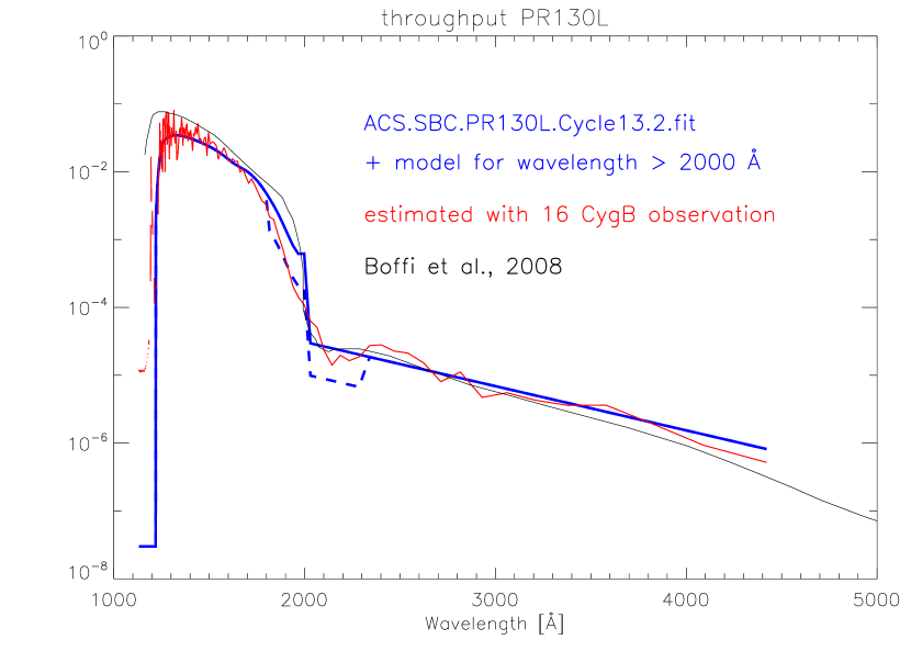
Figure 15: Throughput of the prism PR130L. Blue curve is the calibrated throughput for wavelengths shorter than 2000 Å  from Larson (2006) and modeled with an exponential law for wavelengths larger than 2000 Å  to fit 16 CygB observations. An alternative model for the throughput is used in the paper with a reduced throughput by factor 1/3 within 1800 Å  and 2300 Å  (blue dashed line). Red curve is calculated throughput from 16 CygB observations with solar analog spectrum. We additionally show the total ACS/SBC throughput derived for Synphot by Boffi et al. (2008) in their Figure 3 as thin black line.

We use the observed fluxes displayed in Figure 5 to constrain our model albedo (see Figure 6). We assume a simple linear increase of the model albedo for wavelengths larger than 1700 Å. The quantitative values of this increase has been chosen to match the observed fluxes sufficiently far away from the wavelength ranges which correspond to the O I emission from Europa’s atmosphere (i.e. outside of the vertical dotted and dashed lines). The modeled reflected light is shown as a solid black line in Figure 5, which fits the observations outside of the atmospheric O I wavelengths ranges in general well. However, near the solid vertical line the surface reflected light overestimates the observed fluxes and does not reproduce the ’knee’ in the observations. A principal reason could be a dip in the albedo around 2000 Å. But any uncertainty in the model albedo $a$ can equally well be reflected in an equal uncertainty in the throughput $t$ when working with the prism observations. Only the product of $a$ and $t$ constrains the observed fluxes (see equation (2)). The throughput at wavelengths around and larger than 2000 Å  is also not well constrained (see discussion in Appendix A.1). To improve the fit of the modeled reflected light we introduce a throughput dip of a factor 1/3 within 1800 Å  and 2300 Å  (shown as dashed blue line in Figure 15). This modified throughput leads to a modified spectrum of reflected and dispersed light from the surface of Europa and is displayed as the dashed black line in Figure 5. The spectrum with the throughput dip reproduces the knee in the observed spectrum much better. We will call it in the remainder of this paper ’alternative’ model of reflected surface light. It will provide in subsequent parts of the paper a rough estimate for the consequences of the uncertainties in the model albedo and/or throughput, i.e., it provides an estimate for systematic errors introduced in the subtraction of the reflected light.

At some distance away from the locations of the oxygen images (constrained by the vertical dashed and dotted lines) the observation are close to our modeled reflected light. The surplus of the observed emission compared to the model solar reflected light within and near the dotted and dashed lines is the O I 1356 Å  and O I 1304 Å  radiation emitted from Europa’s atmosphere. It should be noted that in Figure 5 the flux scale is logarithmic, thus a surplus at x=280 appears roughly ten times larger than the same surplus at x=330.

We note that any possible contribution by the geocorona plays a negligible role in our analysis. The O I 1356 Å  of Earth’s atmosphere is below the HST orbit. As we observe Europa near Jupiter opposition, i.e., during HST orbit night, the O I 1304 Å  emission only contributes 1 or 2 Rayleighs uniformly on the detector.

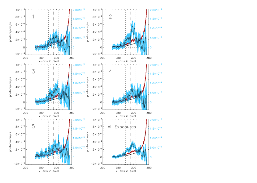
Figure 7: Quantitative comparison of observed fluxes (red) along trace (x-axis) summed along y-axis and modelled solar reflected light (black). The difference between the observed and reflected light is the emission from Europa’s atmosphere shown as black thin line with error bars in blue. The emission from Europa’s atmosphere is multiplied by a factor of five for better visibility (the corresponding values are displayed on the right hand side of each plot, respectively). Vertical dotted lines show area of O I 1304 Å  image and vertical dashed lines displays area of O I 1356 Å  image.

In the next step we display in Figure 7 the observed fluxes for each HST orbit separately. For comparison we also show the modeled solar reflected fluxes. The fluxes are integrated between rows 361 to 385 similar to Figure 5. All error bars include statistical errors only. The signal to noise ratio is calculated by $S/N=(S-B-D)/\sqrt{S+B+D}$ with S and B corresponding to the total counts of the signal and the background, respectively, and D to the total counts of the ACS/SBC dark noise (S, B and D are summed over exposure time and pixel under consideration, respectively). The dark noise count rate is 1.0 $\times 10^{-5}$ cts^-1 s^-1 pixel^-1 Cox (2004). A more detailed representation of the emission from Europa’s atmosphere is given by the integrated fluxes on a linear scale spanning wavelengths below 2000 Å. The solid vertical line in Figure 7 shows the 2000 Å  ’influence line’. The two vertical dashed lines show the locations of the O I 1356 Å  image and the two vertical dotted lines the locations of the O I 1304 Å  image corresponding to the size of Europa’s disk.

The differences between the modeled surface reflected light (black) and the observed fluxes (red) in Figure 7 are due to the emission from Europa’s oxygen atmosphere (blue). We multiplied the values of emission from Europa’s atmosphere by a factor of five to more clearly display it within the individual plots. The corresponding values for the atmospheric emission are shown on the right hand side of each panel in blue. The model fluxes (black) to the right of the O I emission region and to the left of the 2000 Å  influence line match all individual exposures and the superposed exposure (red) fairly well and thus demonstrate that the solar reflected light contributions does not change from orbit to orbit. In contrast, the observed emissions in blue display apparent time-dependence. The observed fluxes change as a function of orbit number as will be analysed in more detail in the following section. The observations also show that there is excess emission beyond the disk of Europa due to the spatial extension of Europa’s atmosphere as visible to the left of the O I 1304 Å  disk, i.e. to the left of the left dotted vertical line. Any excess emission to the right of the O I 1356 Å  disk, i.e. to right of the right vertical dashed line, might be buried within the large error bars in this region. The signal to noise ratio of the radiation from Europa’s atmosphere displayed in Figure 7 is however partially as low as two as apparent in the large error bars. Therefore we will investigate in the remainder of this work areas corresponding to a larger number of pixels for a better signal to noise ratio.

3 Results

3.1 Radial/equatorial structure of atmosphere

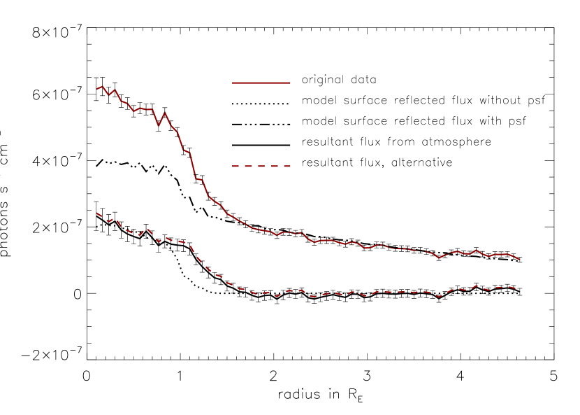
Figure 8: Average emission of Europa’s atmosphere as a function of radial distance from Europa’s center within columns 272 to 326 have been considered.

In Figure 8 we show the average emission as a function of radial distance from the center of the disk of Europa, which we calculate as average emission within thin radial shells of both disks (O I 1304 Å  and 1356 Å). The emission is normalized to the number of pixels in each shell. The radiation within the shells is calculated as the difference in radiation within radius $r+dr$ and of radius $r$. For radial values where the two O I 1304 Å  and 1356 Å  areas overlap, we do not calculate the overlapping part twice. No attempt is made to separate the O I 1304 emissions from the O I 1356 emissions in the overlapping regions. Instead our model instrument response replicates the overlap as part of the fitting process. We restrict ourselves to pixels within columns 274 to 323 in case the shells extend beyond these columns. These columns just embrace the O I 1304 Å  disk to the left and the O I 1356 Å  disk to the right in x-direction. If we were to integrate further to the right in the x-direction (direction of the dispersion) we would also integrate pixels whose emission is significantly contaminated by the red leak. To avoid over-counting the O I 1304 Å  compared to the O I 1356 Å  emission, we do not integrate further to the left of the O I 1304 Å  image. Consequently, the profiles in Figure 8 is more constrained by equatorial than by polar off-disk emission.

The red line in Figure 8 shows the original observations. The dotted line shows the reflected surface light without inclusion of the point spread function. The apparent model emission extends to radial distances larger than 1 R_E even though the surface reflected light is generated within 1 R_E. The reason is that the dispersion of the continuous solar spectrum also generates emission out side of the location of the O I images. The solid black line shows the model surface reflected light including the point spread function. It shows that the scattering of photons within the prism is a significant effect as can be seen in Figure 4 as well. The model reflected light fits the observations at large radial distances remarkably well and thus independently confirms the quality of the constructed point spread function (see Appendix). The difference between the solid red and the black line is the excess emission from Europa’s atmosphere (shown as dashed solid line). It demonstrates non-negligible emission above the disk of Europa which tapers off towards $\sim$1.5 - 1.7$R_{J}$. In Figure 8 we also show the resultant flux from Europa’s atmosphere calculated with the alternative throughput model as red dashed lines. These fluxes differ by only $\sim$10% or less from the fluxes derived with our standard model.

3.2 Atmospheric emission, individual orbits

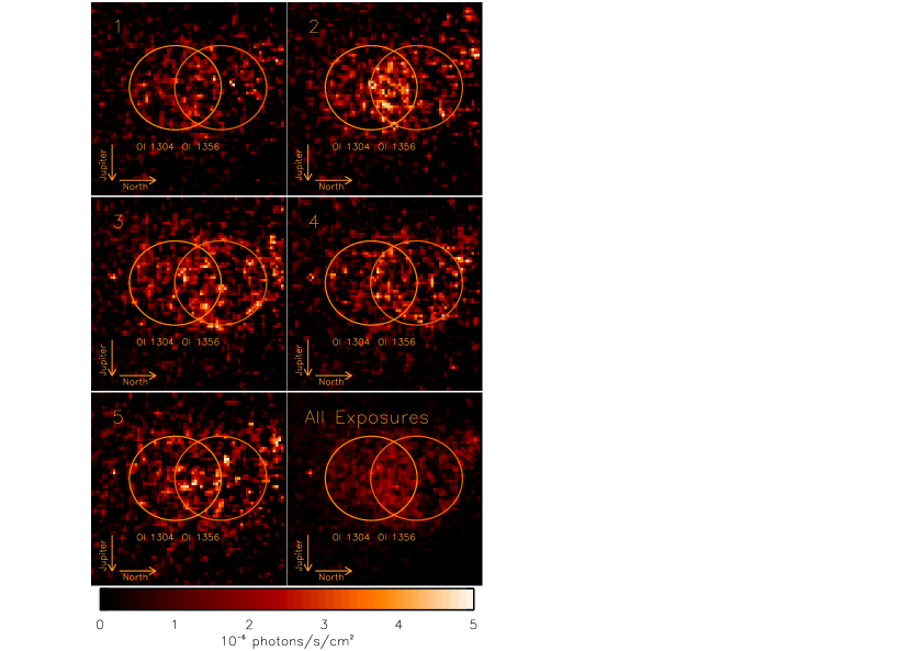
Figure 9: Individual exposures after subtraction of reflected solar light on disk of Europa. North is to the right and Jupiter is down in each image.

The O I 1304 Å  and the O I 1356 Å  emission from Europa’s atmosphere can be reconstructed by subtraction of the reflected and dispersed solar light of the surface from the observations (see Section 2). The emissions from Europa’s atmosphere for all five orbits and the sum of all exposures are shown in Figure 9. The color scale is similar to Figure 2, but enhanced by a factor of 1.5 to more clearly display the flux variations. We note that individual pixels or small cluster of pixels should be interpreted with much caution due to their low signal to noise ratio. The general impression from the images in Figure 9 is that most of the flux occurs within or close to both O I images. The images also show time dependence with orbit 2 and 3 having maximum fluxes. The emission emerges mostly within the disk of Europa, but it also extends beyond the disk as due to a finite atmospheric scale height reported in previous observations Hall et al. (1995); McGrath et al. (2004) and modeling Saur et al. (1998).

3.3 Total fluxes

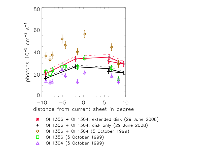
Figure 10: Total fluxes as a function of nominal distance with respect to Jupiter’s magnetic dipole equator. Flux on disk and limb for 2008 June 29 observations ($r<1.3R_{Europa}$). The dashed lines represent the total fluxes when the alternative throughput model is used (see text).

Due to the low signal to noise ratio for individual pixels or small groups of pixels, it is necessary to integrate the emissions over larger areas. Therefore we calculate the total flux from Europa’s atmosphere for each orbit within an extended disk including a radial distance of 1.3 $R_{E}$ from Europa’s center with Europa’s radius $R_{E}$ = 1569 km. In Figure 10 the total fluxes are shown in red as a function of Europa’s position with respect to the current sheet of Jupiter’s magnetosphere. Jupiter’s magnetic moment is tilted with respect to Jupiter’s spin axis by $\sim$9${{}^{\circ}}\;$. Jupiter’s fast rotation period of 9 h and 55 min is responsible for large centrifugal forces, which confine the magnetospheric plasma into a disk around Jupiter’s centrifugal equator, called ’current sheet’ or ’plasma sheet’. The current sheet is close to the magnetic equator while Europa’s orbital plane is within Jupiter’s spin equator. Thus the current sheet rocks above and below Europa within 11.23 h (the synodic rotation period of Jupiter as seen from Europa). Therefore Europa is exposed to different plasma conditions, in particular varying electron densities, within the 11.23 h. This effect is clearly visible in Figure 10. The maximum emission of $\sim$36 $\pm$ 2.2 $\times$ 10^-5 photons cm^-2 s^-1 is reached when Europa is in the center of the current sheet and minimum values of $\sim$21 $\pm$ 2.1 $\times$ 10^-5 photons cm^-2 s^-1 occur when Europa is at the edge of the current sheet. These fluxes correspond to $\sim$230 $\pm$ 14 and $\sim$130 $\pm$ 14 Rayleigh, respectively (see also Table 1). The quoted error bars contain statistical errors only. In Figure 10, we also show the fluxes calculated with the hypothetical dip in the throughput curve as alternative model with dashed lines. The alternative fluxes differ from the standard model by as much as the width of the statistical errors. The difference between the standard and the alternative model can be considered as a rough measure for the systematic error introduced by subtracting the surface reflected light, which contains uncertainties due to the partially unconstrained albedo and red leak.

In black we show the fluxes within the disk of Europa, i.e., within 1 $R_{E}$. The associated values are roughly 3/4 of the fluxes of the extended disk. We note, as both O I images overlap, some of the off disk emission from the real atmosphere falls within the O I disks of the two dispersed O I images. Thus the quoted ratio is an upper limit for the real disk emission.

We can compare the current sheet dependence of the total fluxes to the observations from 1999 October 5 taken with STIS on the trailing side McGrath et al. (2004, 2009). Similarly to the ACS data, we also integrate the STIS data within 1.3 $R_{E}$. The total fluxes from the 1999 October 5 campaign are shown as brown diamonds in Figure 10. The green squares in Figure 10 show the current sheet dependence of the O I 1356 Å  emission and the violet triangles those of the O I 1304 Å  emission. The ratio of the latter two is roughly two to one. The 1999 observations also show a clear dependence on Europa’s position with respect to the current sheet for the O I 1356 Å  emission, while the dependence of the O I 1304 Å  emission is ambiguous. Their total fluxes are roughly 30% to 40% larger than the values derived from the 2008 ACS observations of this work. The combined O I 1356 and O I 1304 fluxes of 137 Rayleigh observed by Hall et al. (1998) with GHRS on the leading side are consistent with the 2008 ACS observations outside of the current sheet and $\sim$50% smaller than the 2008 ACS values when Europa is in the center of the current sheet.

We can use the observed fluxes within the range of 170 to 270 Rayleigh and estimate average column densities. Assuming for simplicity a constant electron density of 40 cm^-3 and temperature of 20 eV similar to Hall et al. (1995) and neglecting the electrodynamic interaction, we can derive a lower limit for the O₂ column density of 6 to 10 $\times$ 10¹⁸ m^-2. Our derived column densities show somewhat less variations, but are still roughly consistent compared to the column densities of 3.5 to 11 $\times$ 10¹⁸ m^-2 derived by Hall et al. (1998). Note that the observed electron density upstream of Europa varies between 18 to 250 cm^-3 Kivelson et al. (2004).

3.4 Search for asymmetries on leading hemisphere

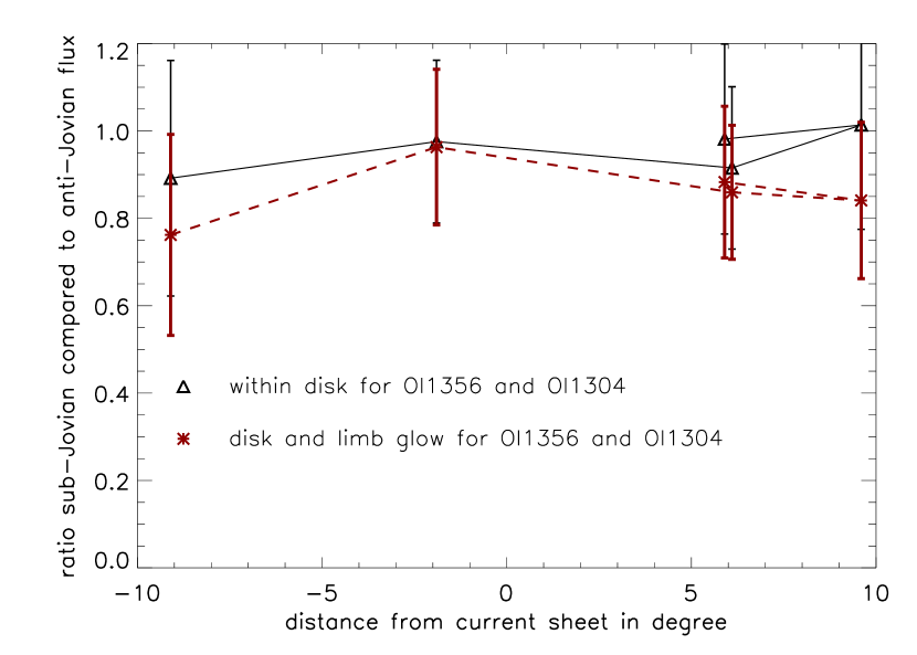
Figure 11: Ratio of sub-Jovian flux compared to anti-Jovian flux for 2008 June 29 observations. For the fluxes within the disk no asymmetry is visible.

The spatially resolved observations of Europa’s atmosphere on the orbital trailing hemisphere in 1999 show a pronounced surplus of emission on the anti-Jupiter side (see Figure 1). We quantitatively searched for similar asymmetries on Europa’s leading hemisphere. Fortunately, the dispersion is in the north-south direction and we can thus well analyze possible asymmetries with respect to the sub-Jovian and anti-Jovian side. In Figure 11, we show the ratio of the total flux within the sub-Jovian side compared to the anti-Jovian side of the emission for each orbit. The black triangles are calculated from the emission within the two O I disks only, while the red stars show the ratio calculated from an extended disk, i.e. within a radius of 1.3 $R_{E}$. The sub-Jovian/anti-Jovian emissions within the disk are within the error bars consistent with a ratio of one, i.e. consistent with a symmetric emission. The extended disk emission shows an average ratio of $\sim$0.9 $\pm 0.2$. Similar to UV observations of Io’s atmospheric emission by Roesler et al. (1999), one might expect the anti-Jovian side of Europa to be brighter due to the Hall effect Saur et al. (1999, 2000). However, this effect is not resolvable within the current error bars. In summary, no sub-Jovian and anti-Jovian asymmetry on the leading side of Europa is visible in contrast to its trailing side.

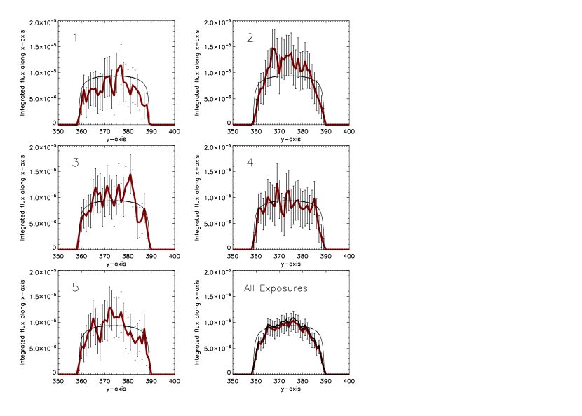
Figure 12: Integrated flux in the x-direction (north south) within the disk of Europa plotted as a function of the y-direction (sub-Jovian/anti-Jovian). Red curve are observations and thin black line is expected radiation from a radially symmetric atmosphere including the point spread function. The black jagged line next to the red one in the lower right panel is calculated with the alternative model (see text).

In a next step we quantitatively search if there is substructure in the emission on the disk of the leading hemisphere. Such a substructure might be generated by inhomogeneities of Europa’s surface properties such as discussed by Cassidy et al. (2007) or plumes speculated by Nimmo et al. (2007a) similar to those observed on Enceladus (e.g., Waite et al., 2006; Spencer et al., 2006; Porco et al., 2006; Dougherty et al., 2006; Hansen et al., 2006; Burger et al., 2007; Saur et al., 2008). Therefore we integrate the fluxes within the disk parallel to the dispersion, i.e. along the x-axis. The resultant integrated fluxes are shown as a function of the sub-Jovian/anti-Jovian direction as red curves plus error bars in thin black for all individual orbits and the sum of all exposures in Figure 12. For comparison we show as black curves the expected emissions from within the disk for a radially symmetric atmosphere with a scale height of 145 km Hall et al. (1995); Saur et al. (1998). The effects of the point spread function on the radially symmetric model atmosphere is included. The model curve for a radially symmetric atmosphere is arbitrarily normalized and displayed to demonstrate possible deviations from a radially symmetric atmosphere in the observed emission in the sub-Jovian/anti-Jovian direction. The observations for the individual orbits show temporal variations in the overall flux. As described in Section 3.3 overall temporal variations of the total intensity are consistent with Europa’s varying position with respect to the current sheet.

We use the sum of all exposures, which combines the O I 1356 Å  and the O I 1304 Å  emission, to investigate possible spatial substructure within the emission. There is more emission near the central meridian (90 degree at eastern elongation) compared to the emission from near the limb as the emission near the limb (near pixel 360 and 390) is smaller compared to the emission profile expected from a radially symmetric atmospheric emission. The observed emission could be consistent with a density enhancement around the 90 degree meridian. Only as an example to characterize the amount of gas, an atmospheric substructure with a radius of $\sim$250 km and a density enhancement by a factor of two to three compared to the background atmosphere would create the observed deviations in Figure 12 compared to a radially symmetric atmosphere. Such density variations could be consistent with model calculations reported by Cassidy et al. (2007). In the right lower panel in Figure 12, which covers the sum of all exposures, we also show the alternative model derived from an alternative throughput curve as a jagged black line close to the jagged red line. It demonstrates that the applied modifications in the throughput does not have qualitative implications on our derived conclusions. We also note that in Figure 12 lower right panel at least four data points close to the limb are within the error bars below the radially symmetric model. We could thus also combine two or all four to a joint point with even smaller error bars.

Nimmo et al. (2007b) suggested that the vapor plumes discovered at Enceladus were caused by tidally-driven shear heating, with the vapor production rate dependent on the local strain rate. If similar shear heating Nimmo & Gaidos (2002) and vapor production occurs at Europa, then the local rate of vapor production should depend on the local strain rate. For a thin ice shell, the time average of the squared tidal strain rate varies spatially, with maxima at the poles and equatorial minima at 0${{}^{\circ}}\;$and 180${{}^{\circ}}\;$west longitude Ojakangas & Stevenson (1989). Figure 13 plots the latitudinal average of this quantity as a function of longitude, demonstrating that strain rates (and hence predicted vapor production) are largest around 90${{}^{\circ}}\;$and 270${{}^{\circ}}\;$west longitude. This analysis is probably over-simplified, in that it assumes the orientation and areal density of shear-heating features is uniform. To take the spatial variation of shear-heating features into account, we also calculated the mean resolved shear stress (a proxy for shear heating rate) on mapped lineaments. The stress calculations are described in the Supplementary Information of Nimmo et al. (2007b) and the lineament map was based on Figure 15b of Kattenhorn & Hurford (2009). Using this approach, we predict a peak in vapor production at 230${{}^{\circ}}\;$west, in striking agreement with the observations on the trailing side reported by McGrath et al. (2004) and shown in Figure 1 of this paper. However, the location of this peak may be an artifact due to the incomplete imaging coverage of polar regions (Doggett et al., 2009, Figure 1.). If the observed peak at 230${{}^{\circ}}\;$west McGrath et al. (2004, 2009) is not a transient feature, and arises because of shear heating, then we predict that future imaging will reveal a paucity of polar ridges around 270${{}^{\circ}}\;$west.

The observed surpluses of O I emission near 90${{}^{\circ}}\;$and in between 200${{}^{\circ}}\;$and 250${{}^{\circ}}\;$west longitude need further investigations. For example, if the surplus O I emission were confined to 1304 Å  and not 1356 Å, it could indicate an optically thick atmosphere in O atoms, which would resonantly scatter solar 1304 Å  photons with enhanced emission at the center of the disk. Hall et al. (1995) used the ’2:1 ratio’ on O I 1356/O I 1304 intensity to put an upper limit on the O atom column density of $<2\times 10^{18}$ m^-2. But this ratio has been observed to be $<$ 2:1 (cf. Hall et al. (1998)) and thus solar 1304 Å  resonance scattering by O atoms may be non-negligible. The observed surpluses also might be due to varying surface properties, such as porosity or albedo. The electrodynamic interaction of Europa’s atmosphere with Jupiter’s magnetosphere will also generate asymmetries in the interaction, however it generally acts to enhance emission on the flanks in contrast to the enhanced emission in the wake. These effects warrant further investigations which are however beyond the scope of this observational paper.

4 Summary and Discussion

Europa’s O I 1304 Å  and 1356 Å  emissions on the leading side observed on 2008 June 29 with ACS/SBC prism PR130L show total fluxes in the range of 130 to 230 Rayleigh. These values are generally comparable with previous observations. They are slightly smaller than fluxes obtained with HST/STIS on the trailing side in the range of 210 to 370 Rayleigh McGrath et al. (2004, 2009), but they are in the range or somewhat larger than previous GHRS observation of 137 Rayleigh on the leading side Hall et al. (1998). The ACS/SBC and the HST/STIS observations demonstrate a clear dependence of the emission depending of Europa’s position relative to Jupiter’s current sheet. We do not find an asymmetry of the atmospheric emission with respect to the sub-Jovian/anti-Jovian side, but find a surplus of emission near 90${{}^{\circ}}\;$west longitude compared to a radially symmetric atmosphere. The previous STIS observations are consistent with a surplus of emission on the trailing side in the range of 200${{}^{\circ}}\;$to 250${{}^{\circ}}\;$west longitude McGrath et al. (2004, 2009). A surplus of emission could be due to a surplus of atmospheric gas, which could be consistent with predictions of possible plume locations on Europa by Nimmo et al. (2007a) near the same longitudes. Other reasons which could contribute to the observed longitudinal enhancement in the UV emission might be intrinsic or solar illumination driven spatial variations of Europa’s ice properties controlling its albedo, porosity and sputtering properties (e.g., Cassidy et al., 2007). For example, the albedo is known to vary with longitude on Ganymede for wavelengths larger than 2200 Å  Nelson et al. (1987); Noll et al. (1995); Hendrix et al. (1998), however it appears to be constant within the error bars in the FUV at 1335 Å  Hall et al. (1998). The emission patterns of Europa’s atmosphere are also controlled by the plasma interaction with Jupiter’s magnetosphere. Europa’s O I 1304 Å  and O I 1356 Å  emissions are generated by electron impact dissociation and are thus a strong function of electron density and temperature. Europa’s leading side is the downstream side of the plasma convection past Europa. Since Europa absorbs the plasma flow including the electrons on its upstream side a rarefied wake of electrons is generated on the downstream, i.e. on the leading side. Additionally, the electron temperatures are decreased compared to the upstream side due to inelastic collisions with Europa’s atmosphere. These effect however rather predicts smaller emission near the 90${{}^{\circ}}\;$west-longitude instead of the observed surplus, but it naturally explains the observed smaller emission from the leading side compared to the trailing disk of Europa.

Europa’s UV emissions are intriguingly puzzling. The limitations caused by the HST/ACS red leak problem and its associated data analysis problems require further observations with HST/STIS at various orbital longitudes and in addition measurements by a possible future Europa orbiter to better understand Europa’s atmospheric emission and its hemispheric differences. Also further numerical simulations are needed to investigate how plumes combined with the time variable plasma interaction possibly control the temporal evolution of Europa’s UV emissions.

Appendix A Appendix: Calibration of prism properties

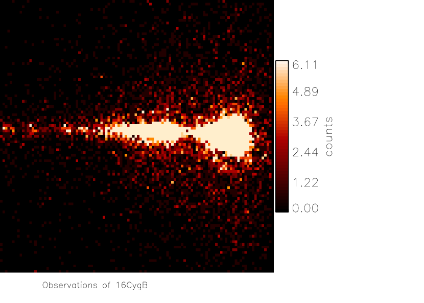
Figure 14: Observations of 16CygB.

For the ACS/SBC prism PRL130, both the throughput for wavelengths larger than 2000 Å  (the red leak) and the point spread function are not available through the calibration pipeline, so we constrain them here. We estimate both properties with observations of 16 CygB, a solar analog star. 16 CygB was observed with ACS/SBC PR130L in Cycle 16 (ID 11325, PI Kuntschner) to improve the existing sensitivity calibrations. In Figure 14 we show observations of 16 CygB dispersed with PR130L. 16 CygB is not a monochromatic point source. In case there were no scattering, the dispersed point source would thus lead to a ’line of emission’ on the detector along the dispersion without spread perpendicular to it (i.e. in our case without spread in the vertical direction in Figure 14). The dispersion and thus the ’line of emission’ is oriented predominantly in the horizontal direction in Figure 14 (similar to our Europa observations). The scattering additionally spreads the emission also to perpendicular to the ’line of emission’. The horizontal direction is also called x-direction and vertical direction the y-direction.

A.1 Long wavelength throughput

The throughput of the prism PR130L for wavelengths larger than 2000 Å  can be estimated with the 16 CygB observations. We employ a solar analog spectrum Woods et al. (1996); Neckel & Labs (1994); Arvesen et al. (1969); Colina et al. (1996) which we disperse as a point source using the dispersion described with formula (2). To retrieve an estimate for the throughput, we integrate the 16 CygB observations along the y-direction on the detector, i.e. collapse the 2D emission onto the ’line of emission’ and divide it by the modeled emission of the solar analog star. The throughput is displayed as a function of wavelength in Figure 15 as the red curve. It agrees fairly well with the calibrated throughput of the prism PR130L for wavelengths shorter than 2000 Å  shown in blue. For wavelengths larger than 2000 Å, our derived throughput serves as basis to construct a model throughput. For $\lambda>$ 2000 Å  we therefore simply use an exponential law which starts at 2000 Å  with a value of a factor of 20 smaller than the calibrated throughput value at $\lambda$ just lower than 2000 Å. It reads

$$t(\lambda)=t_{0}\exp\left[-\frac{\lambda-\lambda_{0}}{H_{red}}\right]$$ (A1)

with $t_{0}$ = 3$\times$10^-5, $\lambda_{0}$ = 2000 Å  and $H_{red}$ = 2000/3 Å. Our model throughput for $\lambda>$ 2000 Å  (blue curve) matches the throughput estimated from the 16 CygB observations (red curve) fairly well. In Figure 15 we also show for comparison the total ACS/SBC throughput rederived by Boffi et al. (2008) for Synphot. In summary, for $\lambda<$ 2000 Å  we use the throughput derived by Bohlin et al. (2000) and for $\lambda>$ 2000 Å  we use as model throughput an exponential law (blue curve in Figure 15).

We also apply a modified, i.e. alternative, throughput in our analysis to study systematic uncertainties in the calculation of the surface reflected light. Therefore we assume a throughput dip in the wavelengths range 1800 Å  to 2300 Å  by factor of 1/3 applied to the model throughput derived in the previous paragraph. The alternative throughput curve is shown as dashed blue line in Figure 15.

A.2 Point Spread Function

We use the 16 CygB observations (ID 11325, PI Kuntschner) also to construct a point spread function (psf) to be used for the Europa observation. Observations of 16 CygB with prism PR130L would lead to a ’line of emission’ on the detector along the dispersion in case there is no scattering. Occurring scattering spreads this line. The scattering is quantified in Figure 16, where we show the observations of 16 Cyg B integrated parallel to the dispersion in the x-direction (columns 268 to 304) as a function of rows (y-direction) as red curve. The observations maximize near row y=432. Near y=432 the flux might be described as a Gaussian, but further away it does not show obvious exponential decay and rather resembles a power law.

To model the observed scatter shown in Figure 16, we use the solar analog spectrum, disperse it with the prism PR130L properties as detailed in (2), and then convolve it with a point spread function to be determined. The scattering as shown in Figure 16 can be modeled by a point spread function of the form

$$\mbox{psf}(x,y)=c_{0}\left[1+\left(\frac{r}{w}\right)^{\gamma}\right]^{-\kappa/\gamma}$$ (A2)

with $r=\sqrt{x^{2}+y^{2}}$. The mathematical expression in (A2) has three free parameters. The first parameter $w$ describes the width of the structure. Its value is related to the full width at half maximum (fwhm) by fwhm $\approx w\times 2^{1+1/\kappa}$ when $\gamma\gg\kappa$. The second parameter $\gamma$ describes the shape of the function around its maximum and the third parameter $\kappa$ models a power law decay further from the maximum. The coefficient $c_{0}$ is introduced such that the two-dimensional integral over the psf renders unity, i.e. $\int\int\mbox{psf}(x,y)\;dx\;dy=1$. This psf resembles a modified version of the $\kappa$-distribution, a well known phase space density function in plasma physics. The $\kappa$-distribution approaches a Gaussian for large $\kappa$ and describes a power law for small $\kappa$. The psf in (A2) turns into an interesting sub-class of point spread functions for $\gamma$=2, and $w=\sigma\sqrt{\kappa}$. In this case (A2) leads to

$$\mbox{psf}(x,y)=c_{0}\left[1+(\frac{r}{\sigma\sqrt{\kappa}})^{2})\right]^{-\kappa/2}\;.$$ (A3)

This psf resembles for finite $\kappa$ a power law with exponent $-\kappa$ for sufficient distances from the source. It turns for large $\kappa$, i.e. in the limit $\kappa\rightarrow\infty$ to a Gaussian with variance $\sigma^{2}$.

We convolve the psf$(x,y)$ in (A2) with the line source calculated with the solar analog spectrum discussed above: The coefficients in the psf are constrained by the integrated 16 CygB measurements shown in Figure 16. We determine the coefficients of the psf quantitatively by fitting it (black curve) to the integrated fluxes along the dispersion (red curve). We find a good fit for $\kappa$ = 2.65, $w$ = 1.17 and $\gamma=20$. For these parameters the derived psf reproduces the 16 CygB observations well, both near the maximum and along the wings (see Figure 16).

Figure 3: Solar spectrum after Woods et al. (1996)

Figure 6: Model albedo for Europa’s leading side as used in our analysis.

s

Figure 13: The time average of the squared tidal strain rate for a thin ice shell (see Ojakangas & Stevenson, 1989, Fig 1), averaged over -90${{}^{\circ}}\;$to 90${{}^{\circ}}\;$latitude and plotted as a function of longitude. Values have been normalized so that the maximum value is 1.

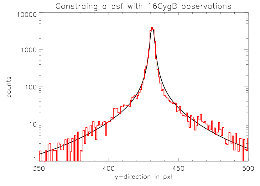
Figure 16: Estimation of the point spread function (psf) in y-direction. Observations of 16CygB in red and model flux to constrain the psf in black.

Table 1: Properties of HST program 11186 executed on 2008-06-29

Orbit	Start time	Exposures	Duration	$\alpha$	Total Flux	Total Flux
	in UT		in s	in degree	in 10-5 photons s-1 cm-2	in Rayleigh	-
1	04:13:14	4	641	-9.1	21 $\pm$ 2.1	132 $\pm$ 14
2	05:48:16	4	641	-1.9	34 $\pm$ 2.2	216 $\pm$ 14
3	07:24:12	4	641	6.1	36 $\pm$ 2.2	226 $\pm$ 14
4	09:00:07	4	641	9.6	29 $\pm$ 2.2	187 $\pm$ 14
5	10:36:02	4	652	8.0	32 $\pm$ 2.2	202 $\pm$ 14

References

- Anderson et al. (2007) Anderson, B. J., Acuña, M. H., Lohr, D. A., Scheifele, J., Raval, A., Korth, H., & Slavin, J. A. 2007, Space Sci. Rev., 131, 417
- Arvesen et al. (1969) Arvesen, J. C., Griffin, Jr., R. N., & Pearson, Jr., B. D. 1969, Appl. Opt., 8, 2215
- Boffi et al. (2008) Boffi, F., Sirianni, M., Lucas, R., Walborn, N., & Proffitt, C. 2008, ISR ACS, 002, 1
- Bohlin et al. (2000) Bohlin, R., Hartig, G., & Boffi, F. 2000, ISR ACS, 001, 1
- Burger et al. (2007) Burger, M. H., Sittler, E. C., Johnson, R. E., Smith, H. T., Tucker, O. J., & Shematovich, V. I. 2007, Journal of Geophysical Research (Space Physics), 112, 6219
- Cassidy et al. (2007) Cassidy, T. A., Johnson, R. E., McGrath, M. A., Wong, M. C., & Cooper, J. F. 2007, Icarus, 191, 755
- Clarke et al. (2002) Clarke, J. T., Ajello, J., Ballester, G. E., Jaffel, L. B., Connerney, J. E. P., Gérard, J.-C., Gladstone, G. R., Grodent, D., Pryor, W., Trauger, J., & Waite, J. H. 2002, Nature, 415, 997
- Colina et al. (1996) Colina, L., Bohlin, R. C., & Castelli, F. 1996, AJ, 112, 307
- Cox (2004) Cox, C. 2004, Instrument Science Report ACS, 014, 1
- Doggett et al. (2009) Doggett, T. et al. 2009, in Europa, ed. R. Pappalardo, W. Mckinnon, & K. Khurana (Tucson Arizona: University of Arizona Press), —
- Dougherty et al. (2006) Dougherty, M. K., Khurana, K. K., Neubauer, F. M., Russell, C. T., Saur, J., Leisner, J. S., & Burton, M. 2006, Science, 311, 1406
- Feldman et al. (2000) Feldman, P. D., McGrath, M. A., Strobel, D. F., Moos, H. W., Retherford, K. D., & Wolven, B. C. 2000, Astrophys. J., 555, 1085
- Feldman et al. (2011) Feldman, P. D., Weaver, H. A., Saur, J., & McGrath, M. A. 2011, in HST Calibration Workshop, ed. S. Deustua & C. Oliveria, Space Telescope Science Institute, 2010
- Greeley et al. (2004) Greeley, R., Chyba, C. F., Head, III, J. W., McCord, T. B., McKinnon, W. B., Pappalardo, R. T., & Figueredo, P. H. 2004, in Jupiter. The Planet, Satellites and Magnetosphere, ed. F. Bagenal, T. E. Dowling, & W. B. McKinnon (Cambridge Univ. Press), 329–362
- Grodent et al. (2006) Grodent, D., Gérard, J., Gustin, J., Mauk, B. H., Connerney, J. E. P., & Clarke, J. T. 2006, Geophys. Res. Lett., 33, L6201
- Hall et al. (1998) Hall, D. T., Feldman, P. D., McGrath, M. A., & Strobel, D. F. 1998, Astrophys. J., 499, 475
- Hall et al. (1995) Hall, D. T., Strobel, D. F., Feldman, P. D., McGrath, M. A., & Weaver, H. A. 1995, Nature, 373, 677
- Hansen et al. (2005) Hansen, C. J., Shemansky, D. E., & Hendrix, A. R. 2005, Icarus, 176, 305
- Hansen et al. (2006) Hansen, C. J. et al. 2006, Science, 311, 1422
- Hendrix et al. (1998) Hendrix, A. R., Barth, C. A., & Hord, C. W. 1998, Icarus, 135, 79
- Hussmann et al. (2002) Hussmann, H., Spohn, T., & Wieczerkowski, K. 2002, Icarus, 156, 143
- Johnson et al. (1982) Johnson, R. E., Lanzerotti, L. J., & Brown, W. L. 1982, Nucl. Instrum. Methods, 198, 147
- Kattenhorn & Hurford (2009) Kattenhorn, S. & Hurford, T. 2009, in Europa, ed. R. Pappalardo, W. Mckinnon, & K. Khurana (Tucson Arizona: University of Arizona Press), 199–236
- Khurana et al. (1998) Khurana, K. K., Kivelson, M. G., Stevenson, D. J., Schubert, G., Russell, C. T., Walker, R. J., & Polanskey, C. 1998, Nature, 395, 777
- Kivelson et al. (2004) Kivelson, M. G., Bagenal, F., Neubauer, F. M., Kurth, W., Paranicas, C., & Saur, J. 2004, in Jupiter, ed. F. Bagenal (University of Colorado: Cambridge Univ. Press), 513–536
- Kivelson et al. (1997) Kivelson, M. G., Khurana, K. K., Joy, S., Russell, C. T., Southwood, D. J., Walker, R. J., & Polanskey, C. 1997, Science, 276, 1239
- Kivelson et al. (2000) Kivelson, M. G., Khurana, K. K., Russell, C. T., Volwerk, M., Walker, J., & Zimmer, C. 2000, Science, 289, 1340
- Kliore et al. (1997) Kliore, A. J., Hinson, D. P., Flasar, F. M., Nagy, A. F., & Cravens, T. E. 1997, Science, 277, 355
- Lagg et al. (2003) Lagg, A., Krupp, N., Woch, J., & Williams, D. J. 2003, Geophys. Res. Lett., 30, 4039
- Larson (2006) Larson, S. 2006, ST-ECF Instrument Science Report ACS, 02, 1
- Liu et al. (2001) Liu, Y., Nagy, A., Kabin, K., Combi, M., DeZeeuw, D., Gobmosi, T., & Powell, K. 2001, Geophys. Res. Lett., 27, 1791
- Mauk et al. (2003) Mauk, B., Mitchell, D., Krimigis, S., Roelof, E., & Paranicas, C. 2003, Nature, 412, 920
- McGrath et al. (2009) McGrath, M., Hansen, C., & Hendrix, A. 2009, in Europa, ed. R. Pappalardo, W. Mckinnon, & K. Khurana (Tucson Arizona: University of Arizona Press), —
- McGrath et al. (2004) McGrath, M., Lellouch, E., Strobel, D., Feldman, P., & Johnson, R. 2004, in Jupiter, ed. F. Bagenal (University of Colorado: Cambridge Univ. Press), 457–485
- Neckel & Labs (1994) Neckel, H. & Labs, D. 1994, Sol. Phys., 153, 91
- Nelson et al. (1987) Nelson, R., Lane, A., Matson, D., Veeder, G., Buratti, B., & Tedesco, E. 1987, Icarus, 72, 358
- Neubauer (1998) Neubauer, F. M. 1998, J. Geophys. Res., 103, 19843
- Neubauer (1999) —. 1999, J. Geophys. Res., 104, 28671
- Nimmo & Gaidos (2002) Nimmo, F. & Gaidos, E. 2002, Journal of Geophysical Research (Planets), 107, E5021
- Nimmo et al. (2007a) Nimmo, F., Pappalardo, R., & Cuzzi, C. 2007a, AGU Fall Meeting Abstracts
- Nimmo et al. (2007b) Nimmo, F., Spencer, J., Pappalardo, R., & Mullen, M. 2007b, Nature, 447, 289
- Noll et al. (1995) Noll, K. S., Weaver, H. A., & Gonnella, A. 1995, J. Geophys. Res., 1000, 19,057
- Ojakangas & Stevenson (1989) Ojakangas, G. W. & Stevenson, D. J. 1989, Icarus, 81, 220
- Pappalardo et al. (1999) Pappalardo, R. T. et al. 1999, J. Geophys. Res., 104, 24015
- Porco et al. (2006) Porco, C. et al. 2006, Science, 311, 1393
- Pospieszalska & Johnson (1989) Pospieszalska, M. K. & Johnson, R. E. 1989, Icarus, 78, 1
- Roesler et al. (1999) Roesler, F. L., Moos, H. W., Oliversen, R. J., Woodward, R. C., Retherford, K. D., Scherb, F., McGrath, M. A., Smyth, W. H., Feldman, P. D., & Strobel, D. F. 1999, Science, 283, 353
- Saur (2004) Saur, J. 2004, J. Geophys. Res., 109, A01210
- Saur et al. (2010) Saur, J., Neubauer, F. M., & Glassmeier, K.-H. 2010, Space Sci. Rev., 152, 391
- Saur et al. (1999) Saur, J., Neubauer, F. M., Strobel, D. F., & Summers, M. E. 1999, J. Geophys. Res., 104, 25105
- Saur et al. (2000) —. 2000, Geophys. Res. Lett., 27, 2893
- Saur et al. (2008) Saur, J., Schilling, N., Neubauer, F. M., et al. 2008, Geophys. Res. Lett., 35, L20105
- Saur et al. (1998) Saur, J., Strobel, D. F., & Neubauer, F. M. 1998, J. Geophys. Res., 103, 19947
- Schilling et al. (2007) Schilling, N., Neubauer, F. M., & Saur, J. 2007, Icarus, 192, 41
- Schilling et al. (2008) —. 2008, J. Geophys. Res., 113, A03203
- Shematovich et al. (2005) Shematovich, V. I., Johnson, R. E., Cooper, J. F., & Wong, M. C. 2005, Icarus, 173, 480
- Shi et al. (1995) Shi, M., Baragiola, R. A., Grosjean, D. E., Johnson, R. E., Jurac, S., & Schou, J. 1995, J. Geophys. Res., 100, 26387
- Spencer et al. (2006) Spencer, J. et al. 2006, Science, 311, 1401
- Waite et al. (2006) Waite, J. et al. 2006, Science, 311, 1419
- Woods et al. (1996) Woods, T. N., Prinz, D. K., Rottman, G. J., London, J., Crane, P. C., Cebula, R. P., Hilsenrath, E., Brueckner, G. E., Andrews, M. D., White, O. R., VanHoosier, M. E., Floyd, L. E., Herring, L. C., Knapp, B. G., Pankratz, C. K., & Reiser, P. A. 1996, J. Geophys. Res., 101, 9541
- Zimmer et al. (2000) Zimmer, C., Khurana, K., & Kivelson, M. 2000, Icarus, 147, 329
s