Two-Photon Exchange Effect Studied with Neural Networks

Abstract

An approach to the extraction of the two-photon exchange (TPE) correction from elastic $ep$ scattering data is presented. The cross section, polarization transfer (PT), and charge asymmetry data are considered. It is assumed that the TPE correction to the PT data is negligible. The form factors and TPE correcting term are given by one multidimensional function approximated by the feed forward neural network (NN). To find a model-independent approximation the Bayesian framework for the NNs is adapted. A large number of different parametrizations is considered. The most optimal model is indicated by the Bayesian algorithm. The obtained fit of the TPE correction behaves linearly in $\epsilon$ but it has a nontrivial $Q^{2}$ dependence. A strong dependence of the TPE fit on the choice of parametrization is observed.

I Introduction

The study of elastic $ep$ scattering provides an opportunity to explore the structure of the proton. From $ep$ cross section data the magnetic ($G_{M}$) and electric ($G_{E}$) proton form factors (FFs) are obtained via longitudinal-transverse (LT) separation Perdrisat:2006hj ; Arrington:2006zm . In the data analysis, it is convenient to consider the reduced cross section, which in the one-photon exchange (OPE) approximation, reads as

$$\sigma_{1\gamma,R}(Q^{2},\epsilon) = \tau G_{M}^{2}(Q^{2})+\epsilon G_{E}^{2}(Q^{2}),$$ (1)

$$\tau=Q^{2}/4M^{2},\; \epsilon=\left(1+2(1+\tau)\tan^{2}(\theta/2)\right)^{-1},$$

where $Q^{2}$ and $\theta$ are the four-momentum transfer squared and scattering angle respectively.

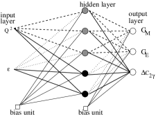
Figure 1: The 2-(3-2)-3 type network, two input units, one layer of hidden units, and three output units. The FF sector (gray filled units and dashed connections) in contrast to the TPE sector (black units and solid connections) is connected only with $Q^{2}$. Dotted lines denote the switched-off connections. Solid and dashed lines represent the weight parameters. The bias unit is not connected with the units from the previous layer, and its signal is equal to 1, which means that $f_{act}^{bias}=1$.

The FF ratio,

$$\mathcal{R}_{1\gamma}(Q^{2})=\mu_{p}\frac{G_{E}(Q^{2})}{G_{M}(Q^{2})}$$ (2)

($\mu_{p}$, the magnetic moment of the proton) can be extracted from the so-called polarization transfer (PT) measurements Ron:2011rdand_Puckett:2011xg . It turns out that the systematic discrepancy between the FF ratio data obtained via the LT separation and the PT measurements exists. It seems that taking into account the two-photon exchange (TPE) correction, the one which is not included in the classical treatment of the radiative corrections Mo:1968cg , cancels this discrepancy Guichon:2003qm ; Blunden:2003sp . Moreover, it is claimed that TPE correction to the $\mu_{p}G_{E}/G_{M}$ ratio, extracted from the PT measurements, is negligible Guichon:2003qm ; Meziane:2010xc . However, taking into account the TPE contribution, in the LT separation, affects significantly the extracted values of the proton FFs. The reduced cross section is modified by the TPE correction $\Delta C_{2\gamma}(Q^{2},\epsilon)$, namely,

$$\sigma_{1\gamma+2\gamma,R}(Q^{2},\epsilon)=\sigma_{1\gamma,R}(Q^{2},\epsilon)+\Delta C_{2\gamma}(Q^{2},\epsilon).$$ (3)

The TPE effect has been studied extensively during the past few years, for reviews and references, see Refs. Carlson:2007sp ; Arrington:2011dn . The recent studies can be found in Refs. Meziane:2010xc ; Qattan:2011zz ; Borisyuk:2010ep ; Guttmann:2010au .

The dominant part of $\Delta C_{2\gamma}(Q^{2},\epsilon)$ is given by the interference between the OPE and the TPE amplitudes. Hence, for the $e^{+}p$ scattering,

$$\Delta C_{2\gamma}(e^{+}p)=-\Delta C_{2\gamma}(e^{-}p).$$ (4)

Therefore, the magnitude of the TPE term can be evaluated by measuring the ratio of the $e^{+}p$ to $e^{-}p$ elastic cross sections positron data ; Yount62 ,

$$\mathcal{R}_{\pm}(Q^{2},\epsilon)=1-\frac{2\Delta C_{2\gamma}(Q^{2},\epsilon)}{\sigma_{1\gamma+2\gamma,R}(Q^{2},\epsilon)}.$$ (5)

A deviation of this function from unity indicates the importance of the TPE effect Arrington:2003ck .

A direct prediction of the proton FFs and TPE correction is a difficult task. One has to deal with the problems of quantum chromodynamics in the non-perturbative regime. The successful approaches are rather phenomenological, and contain many internal parameters, which are fixed to reproduce the experimental data (for reviews see Refs. Perdrisat:2006hj ; Arrington:2006zm ; Arrington:2011dn ).

On the other hand, the existing elastic polarized and unpolarized $e^{-}p$ and $e^{+}$p scattering data cover kinematical region broad enough to reconstruct the FFs dependence on $Q^{2}$. To combine the cross section data with the PT measurements and the $e^{-}p/e^{+}$p ratio data allows one to obtain information about the TPE contribution.

The aim of this paper is to find the approximation of the FFs and the TPE contribution by mainly relying on the experimental data. We reduce the model-dependent assumptions to the necessary minimum.

Figure 2: Logarithm of evidence, see Eq. (24). Each single point, in the plot, represents the ln(evidence) obtained for one particular NN architecture.

II TPE and Neural Networks

Only three complex FFs, which depend on $Q^{2}$ and $\epsilon$, are required to describe the elastic unpolarized and polarized $ep$ Guichon:2003qm scattering amplitudes. Hence, six real functions have to be determined from the data.

We assume that the PT ratio data are not affected by the TPE effect. Then, one can show that only three unknown functions have to be found: two proton FFs and the $\Delta C_{2\gamma}$ correcting term [see Eq. (3)]. Analyses with similar TPE assumptions have been performed by many groups Chen:2007ac ; Rekalo:2003xa ; Borisyuk:2007re ; TomasiGustafsson:2004ms ; Arrington:2004ae ; Arrington:2007ux ; Alberico:2008sz ; Arrington:2003df .

In this paper, we consider the cross section, the PT, and the $e^{+}p/e^{-}p$ ratio data. To consider at least three different data types appeared to be necessary because of the limited model assumptions about the TPE term.

To approximate the FFs and TPE function one has to assume particular empirical parametrization. However, it is obvious that the choice of the functional form of the parametrization has an impact on the fit and its uncertainties. In particular, it is the case of the TPE contribution. This problem was not discussed in the previous analyses.

In the approach presented in this paper, fitting the data means the construction of the statistical model with the ability to predict the FFs and the TPE term. We apply the methods of the Bayesian statistics, which allows performing a model comparison. Indeed, we consider as many different data parametrizations as possible, and the best model is indicated by the objective Bayesian procedure.

In practice, one has to evaluate the probability distribution $\mathcal{P}(model)$ in the space of all functional parametrizations of the FFs and the TPE contribution. The best model should maximize this probability.

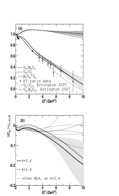
Figure 3: (a) (Top panel) $G_{E}/G_{D}$, $G_{M}/\mu_{p}G_{D}$ [$G_{D}=1/(1+Q^{2}/0.71~{}\mathrm{GeV}^{2})^{2}$] and ratio $\mu_{p}G_{E}/G_{M}$. The predictions of the proton FFs of Arrington et al. Arrington:2007ux also are shown. The PT $\mu_{p}G_{E}/G_{M}$ data are taken from Refs. Ron:2011rdand_Puckett:2011xg ; Puckett:2010ac ; Meziane:2010xc . Shaded areas denote $1\sigma$ uncertainty. (b) (Bottom panel) The $Q^{2}$ dependence of $\Delta C_{2\gamma}/\sigma_{1\gamma+2\gamma,R}$ at $\epsilon=$0.4 and 0.8. The shaded area denotes $1\sigma$ uncertainty computed for the fit at $\epsilon=0.4$. The dotted lines denote the TPE term predicted at $\epsilon=$ 0.4 by the networks that have lower than best-fit evidence values.

It is obvious that the magnetic and electric FFs as well as the TPE correction function are correlated. All of them should be determined by the same underlying fundamental model. Therefore, one can imagine that there exists a multidimensional function, defined by the set of parameters, which simultaneously describe all $G_{M}$, $G_{E}$ and $\Delta C_{2\gamma}$. In this paper, we use the artificial neural networks (ANNs) to approximate this function. We consider a particular type of ANN, the feed forward neural network (NN) in the so-called multi layer perceptron (MLP) configuration.

The experimental data, which are analyzed here, depend on either one (only $Q^{2}$) or two ($Q^{2}$ and $\epsilon$) kinematical variables. Hence, the MLP must map two-dimensional input space [$\vec{\mathrm{in}}=(Q^{2},\epsilon)^{T}$] to output space, spanned by three functions $\vec{\mathrm{out}}=(G_{M},G_{E},\Delta C_{2\gamma})^{T}$.

We consider MLP networks that consist of three layers of units: input, hidden layer, and output (see Fig. 1). Each single neuron (unit) of the network calculates its output value as an activation function $f_{act}$ of the weighted sum of its inputs $f_{act}\left(\sum_{i}w_{i}\mu_{i}\right)$, where $w_{i}$ denotes the i-th weight parameter, while $\mu_{i}$ represents the output value of the unit from the previous layer.

For the activation functions we take the sigmoid $sigmoid(w)=1/(1+\exp(-w))$ and the linear functions for the hidden and output units, respectively. It has been proven Cybenko_Theorem that the maps given by the networks with one hidden layer and with the sigmoid like activation functions, in this layer, are sufficient to approximate any continuous real function. Indeed, we assume that the FFs and TPE term are the continuous functions of kinematical variables. Notice that the efficiency of approximation depends on the number of hidden units. In some problems it might be a very large number.

Additionally let us mention a useful property of the sigmoid function. Its effective support is concentrated in the close neighborhood of $w=0$. With increasing $|w|$, the sigmoid saturates. This property allows restricting the effective range of the weight parameters.

The $G_{M}$ and $G_{E}$ only depend on $Q^{2}$. This property is achieved by the particular choice of the architecture of MLP, namely some of the connections are erased. As a result, the network is divided into two sectors. One, called the latter FF sector, which is disconnected with the $\epsilon$ input and the second, called the latter TPE sector, which is connected with both input values. The FFs and TPE correction are still determined by the large subset of common weights.

An example of the 2-(3-2)-3 network ($\mathcal{A}_{3,2}$) is drawn in Fig. 1. It consists of two input units, five units in the hidden layer (three units belong to the FF sector, and two units belong to the TPE sector), and 3 output units.

The choice of the particular configuration of units and number of the hidden units, defines the network architecture $\mathcal{A}_{g,t}$. For given $\mathcal{A}_{g,t}$ the particular map $\mathcal{N}_{g,t}$ is defined as

$$\mathcal{N}_{g,t}:\mathbb{R}^{2}\mapsto\mathbb{R}^{3},\quad\mathcal{N}_{g,t}(Q^{2},\epsilon;\mathcal{A}_{g,t},\vec{w})=\pmatrix{G_{M}\cr G_{E}\cr\Delta C_{2\gamma}}.$$ (6)

To have network $\mathcal{A}_{g,t}$, the optimal values of the weight parameters have to be found. The process of establishing them is called the training of the network and it is described in the next part of the paper.

It is obvious that, to find the optimal network architecture, which approximates desired map well, the number of hidden units has to be varied. In this paper we apply the method that allows estimating the optimal size of the hidden layer.

III Bayesian Framework

The MLPs with a larger number of units (with many weights) have a better ability to represent the data. However, usually too complex parametrizations exactly resemble the data and usually tend to reflect the statistical fluctuations. Thus, the generality of the description is lost, and the data are over-fitted. Moreover, the complex parametrizations may lead to larger uncertainties than the simple models. On the other hand, too simple parametrizations are not capable of coding all the important information hidden in the measurements. The fits described by the simple functions might be characterized by the underestimated uncertainties.

A task of finding the optimal statistical model that represents the data accurately enough but does not overfit the data is known in statistics as the bias-variance trade off problem. In the previous global analyses of the $ep$ data the degree of the complexity of the FFs and TPE parametrizations was chosen with the help of phenomenological arguments and common sense. In this paper, we wish to apply the objective Bayesian methods, which allow quantitatively investigating the complexity of the FFs and TPE correcting functions.

The Bayesian framework (BF) formulated for the NN computations bayes faces the problems described above. This approach has already been adapted to approximate the electromagnetic nucleon FFs Graczyk:2010gw and, here, it is developed to study the TPE effect. The BF was designed to:

• quantitatively classify the statistical hypothesis;

• objectively choose the best network architectures and consequently, the number of hidden units;

• find the optimal values of the weight parameters;

• objectively establish the training parameters, such as the regularization parameter $\alpha$ (it will be explained below).

Notice that to deal with the overfitting problem one can also use the cross-validation technique. It is complementary approach which has been applied by the NNPDF group for fitting the parton distribution functions Ball:2010de .

At the beginning of the Bayesian analysis, we assume that all possible models are equally likely,

$$\mathcal{P}(\mathcal{A}_{1,1})=...=\mathcal{P}(\mathcal{A}_{g,t})=...,$$ (7)

where $\mathcal{P}(\mathcal{A}_{g,t})$ denotes the prior probability.

With the help of Bayes’ theorem the posterior probability for a given model (network) is obtained as

$$\mathcal{P}(\mathcal{A}_{g,t}|\mathcal{D})=\frac{\mathcal{P}(\mathcal{D}|\mathcal{A}_{g,t})\mathcal{P}(\mathcal{A}_{g,t})}{\mathcal{P}(\mathcal{D})},$$ (8)

where $\mathcal{D}$ is the experimental data, $\mathcal{P}(\mathcal{A}_{i}|\mathcal{D})$ is the probability of the model given data $\mathcal{D}$, and $\mathcal{P}(\mathcal{D})$ is some constant real number. Because of the prior assumption (7), it is obvious that, to classify the hypothesis, it is enough to evaluate the evidence $\mathcal{P}(\mathcal{D}|\mathcal{A}_{g,t})$–the probabilistic measure of goodness of fit.

For given network architecture $\mathcal{A}_{g,t}$, the optimal $\vec{w}_{MP}$ weight parameters should maximize the posterior probability,

$$\mathcal{P}\left(\vec{w}\right|\left.\mathcal{D},\{\mathcal{I}\},\mathcal{A}_{g,t}\right)=\frac{\mathcal{P}\left(\mathcal{D}\right|\left.\vec{w},\{\mathcal{I}\},\mathcal{A}_{g,t}\right)\mathcal{P}\left(\vec{w}\right|\left.\{\mathcal{I}\},\mathcal{A}_{g,t}\right)}{\mathcal{P}\left(\mathcal{D}\right|\left.\{\mathcal{I}\},\mathcal{A}_{g,t}\right)},$$ (9)

where $\mathcal{P}\left(\mathcal{D}\right|\left.\vec{w},\{\mathcal{I}\},\mathcal{A}_{g,t}\right)$ is the likelihood function of the data, $\mathcal{P}\left(\vec{w}\right|\left.\{\mathcal{I}\};\mathcal{A}_{g,t}\right)$ denotes the prior probability, and $\{I\}$ denotes the set of initial constraints.

The data likelihood function is defined by

$$\mathcal{P}(\mathcal{D}|\vec{w},\{\mathcal{I}\},\mathcal{A}_{g,t})\sim\exp\left(-S_{ex}(\mathcal{D},\vec{w})\right),$$ (10)

where

$$S_{ex}(\mathcal{D},\vec{w})=\chi^{2}_{\sigma}+\chi^{2}_{PT}+\chi^{2}_{\pm}+\chi_{G_{M}}^{2}+\chi_{G_{E}}^{2}$$ (11)

is the experimental error function. By $\chi^{2}_{\sigma,PT,\pm}$, we denote the error functions of the cross section (16), the PT (17) and the $e^{+}p/e^{-}p$ ratio (18) data. Eventually, $\chi_{G_{M/E}}^{2}$ denotes the error function introduced to take the two artificial FF points into account (see the discussion below).

We distinguish between the ANN and the physical initial constraints $\{\mathcal{I}\}=\{\mathcal{I}\}_{ANN}\cup\{\mathcal{I}\}_{phys.}$.

The ANN constraints $\{\mathcal{I}\}_{ANN}$ are introduced to face the overfitting problem. Indeed, defining the prior probability as follows:

$$\mathcal{P}\left(\vec{w}\right|\left.\{\mathcal{I}\}_{ANN},\mathcal{A}_{g,t}\right) = \mathcal{P}\left(\vec{w}\right|\left.\alpha,\mathcal{A}_{g,t}\right)\sim\exp\left(-\alpha E_{w}(\vec{w})\right)$$

$$E_{w}(\vec{w}) = \frac{1}{2}\sum_{i\in all\,weights}w^{2}_{i}$$ (13)

prevents getting the overfitted parametrizations.

The physical constraints $\{\mathcal{I}\}_{phys.}$ are motivated by the general properties of the FFs and the TPE term Rekalo:2003xa ; Chen:2007ac . We assume that, at $Q^{2}=0$, $G_{M}/\mu_{p}=G_{E}=1$ and $\Delta C_{2\gamma}(\epsilon=1)=0$. In practice, three artificial data points are added to the experimental data sets, namely, [$G_{M}(0)/\mu_{p}=1,\Delta G_{M}(0)=\Delta$], [$G_{E}(0)=1,\Delta G_{M}(0)=\Delta$], and [$\mathcal{R}_{\pm}(0,1)=1,\Delta\mathcal{R}_{\pm}(0,1)=\Delta$], where $\Delta=0.01$. The influence of the $\Delta$ value on the fits and the training process were investigated in the preliminary stage of the analysis. It was obtained that, with $\Delta<0.01$, the efficiency of the training process was very low, while retaining $\Delta>0.01$ was not sufficient to attract the fit for the desired value at the constraint points.

One can show that the maximum of the posterior probability (9) corresponds to the minimum of the total error function,

$$S_{ex}(\mathcal{D},\vec{w})+\alpha E_{w}(\vec{w}).$$ (14)

Let $\vec{w}_{MP}$ denote the weight configuration, which minimizes the above expression. To find the minimum (14), the quick-prop gradient descent algorithm quick-prop , is applied. The weight parameters are updated iteratively, because of the algorithm, until the minimum is reached.

The proper choice of the $\alpha$ parameter is crucial for getting the fits and for further model comparison. If the $\alpha$ parameter is small then the penalty term (13) does not significantly affect the results of the training process. In the language of the Bayesian statistics, a small $\alpha$ value corresponds to the large width of the prior probability distribution (III).

The BF provides a recipe on how to establish the optimal $\alpha$ parameter. For the optimal $\alpha_{MP}$ and $\vec{w}_{MP}$ the probability distribution,

$$\mathcal{P}\left(\alpha\right|\left.\mathcal{D},\mathcal{A}_{g,t}\right)=\frac{\mathcal{P}\left(\mathcal{D}\right|\left.\alpha,\mathcal{A}_{g,t}\right)\mathcal{P}\left(\alpha\right|\left.\mathcal{A}_{g,t}\right)}{\mathcal{P}\left(\mathcal{D}\right|\left.\mathcal{A}_{g,t}\right)}$$ (15)

is maximized.

From the above expression, one can obtain, the necessary condition (22), which has to be satisfied by $\alpha_{MP}$. In this version of the BF approach, we consider the so-called ladder approximation, where the expression (22) is used to iteratively update the $\alpha$ value (during the training process), as long as it converges. In reality, because Eq. (22) is valid in the neighborhood of the minimum, the $\alpha$ parameter is not changed until the training process approaches the close surrounding of the minimum. In this part of the training $\alpha_{0}$ is fixed and equals 0.01. Then, it starts to be updated.

In general, for every weight parameter, one would introduce its own regularization factor. However, notice that $\alpha$ is an example of the scale parameter of the model, given that network $\mathcal{A}_{g,t}$ is symmetric under the permutation of units in the hidden layer.. This property allows reducing the number of independent regularization parameters to six: three in the FF sector (hidden, bias, and linear regularization factors) and three in the TPE sector (similar to before). On the other hand, $\Delta C_{2\gamma}$ is given by the linear combination of the nucleon FFs, multiplied by the additional TPE-like FFs (see Eq. (14) of Ref. Carlson:2007sp ). It means that, if the parameters of the FF sector are scaled, then the weights of the TPE sector should also be rescaled. This property only seems to be approximate, but we use it to reduce the number of regularization parameters to three. Eventually, we noticed that in our previous paper, it was shown that it was enough to consider one regularization parameter to fit the FF data Graczyk:2010gw . Hence, to simplify the numerical calculations and also to accelerate the training process (more than 45 000 training processes have been performed), we consider the simplest regularization scenario with one $\alpha$ parameter. However, as described above, this part of the approach can be improved future .

By having the optimal values of the weight and $\alpha$ parameters the evidence is computed from Eq. (24) The logarithm of evidence is given by two main contributions: the misfit of the approximate data (the experimental error function at the minimum) and the Occam factor. The latter penalizes complex models. The most optimal model has the highest value of evidence. The evidence formula and the description of its properties can be found in Appendix D.

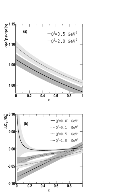
Figure 4: (a) (Top panel) Ratio $\mathcal{R}_{\pm}$ predicted by the network 2-(5-6)-3. The grey areas denote $1\sigma$ uncertainty. (b) (Bottom panel) $\Delta C_{2\gamma}/G_{D}^{2}$ dependence on $\epsilon$. The darker and lighter gray areas denote $1\sigma$ uncertainty.

IV Numerical Analysis

As mentioned in the previous section, we consider three types of measurements: the cross section (27 sets), the PT (14 sets) and the $e^{+}p/e^{-}p$ ratio (3 sets) data.

The selection of the cross section and PT ratio data sets is the same as in one of our previous papers Alberico:2008sz . However, in the case of the PT data, two data sets are replaced with their recent updates Ron:2011rdand_Puckett:2011xg . Additionally, we also include the latest PT measurements of the FF ratio Meziane:2010xc ; Puckett:2010ac . Since the presence of the PT ratio data is required to properly extract the TPE contribution, we only consider the cross section points below $Q^{2}=10$ GeV². Above this limit, the PT data are not available.

In the case of the cross section data, similar to Ref. Alberico:2008sz , the systematic normalization uncertainties are taken into account. For every data set, a normalization parameter is introduced and it is established during training. The procedure is described in Appendix B.

We consider the networks of type 2-(g-t)-3, where $4\leq g+t=M\leq 12$. In the preliminary stage of the analysis, it has been observed that the networks with either g=1, or t=1 have not been able to approximate the data well (similar to the networks with $M<4$). Therefore we only consider models with $g,t>1$. Finally we discuss 45 different ANN architectures. For every network $\mathcal{A}_{g,t}$ type $10^{3}$ networks, with randomly chosen initial values of weights, have been trained. Among them, the parametrization with the highest evidence was used for further model comparison. It turned out that the highest evidence value was obtained for network 2-(5-6)-3 (see Fig. 2).

In Fig. 3(a), we plot the FF ratio $\mathcal{R}_{1\gamma}$ computed with the network $\mathcal{A}_{5,6}$ (our best fit). The shaded areas denote $1\sigma$ uncertainty computed from the covariance matrix of the fit. Our predictions of the FFs are compared to the results of Ref. Arrington:2007ux where the TPE function was postulated based on the phenomenological arguments. The discrepancy between our fits and those of Ref. Arrington:2007ux appears above $Q^{2}$=4 GeV².

In Fig. 3(b), the $Q^{2}$ dependence of ratio $\Delta C_{2\gamma}/\sigma_{1\gamma+2\gamma}$ is presented. We see that at $Q^{2}\sim 0.2$ GeV² the TPE correcting term has a local minimum and it becomes the decreasing function of $Q^{2}$ above 2 GeV². With growing $Q^{2}$, fit uncertainty also enlarges. Indeed, above $Q^{2}=6$ GeV², the number of experimental points is limited and the data are not accurate enough to get an exact approximation. It is interesting to mention that, for large $\epsilon$ (above 0.8) and $Q^{2}$ around 1.5 GeV², the TPE correction is positive.

In Fig. 3(b), we also plot the TPE contribution (dotted lines) predicted by the models: $\mathcal{A}_{4,2}$, $\mathcal{A}_{4,3}$, $\mathcal{A}_{6,2}$, $\mathcal{A}_{6,3}$, $\mathcal{A}_{6,4}$, and $\mathcal{A}_{5,7}$. They are characterized by lower evidence values than the $\mathcal{A}_{5,6}$ model, but they could be acceptable because of the $\chi^{2}$ method (their $\chi^{2}_{min}$ values are much lower than the number of points). The difference between these fits and the prediction of $\mathcal{A}_{5,6}$ is spectacular. It demonstrates that the model comparison is crucial for the proper choice of TPE parametrization.

By keeping the forthcoming measurements of the elastic $e^{-}p$ and $e^{+}p$ scatterings positron_new in mind, in Fig. 4(a), we plot our predictions of ratio $\mathcal{R}_{\pm}$. Although, we have not assumed the linearity of the TPE term in $\epsilon$, the final fit behaves like a linear function of $\epsilon$, as observed in the previous global analysis Tvaskis:2005ex . Although nonlinearities appear at the low $\epsilon$ and $Q^{2}$ values (bottom panel of Fig. 4), in this kinematical domain, the fits have large uncertainties, and the obtained results are in agreement with the linear approximation.

The obtained TPE function has a particular analytical form (see Appendix E), which can be written as the Taylor series in $\epsilon$. If one neglects higher rather than linear $\epsilon$ terms, then the TPE correction is the sum of two contributions, which play a particular role in the LT separation. One of them corrects the magnetic FF, and it appears to be negative. The other modifies the electric FF, and it is the positive function of $Q^{2}$.

Notice that the PT data are not present below $Q^{2}=0.16$ GeV². Hence its influence on the extraction of the TPE in this kinematical range is small. Although because of the lack of PT data, the TPE is still constrained in the low $Q^{2}$ region. Namely, there are several $e^{+}p/e^{-}p$ ratio data points Yount62 . Additionally, we keep one artificial point at $Q^{2}=0$, and $\epsilon=1$ which constrains $\Delta C_{2\gamma}$. Also, there are plenty of cross section data points and the two artificial FF points. The presence of the FF points determines the low $Q^{2}$ behavior of the $\sigma_{1\gamma,R}$. All together, provides restrictions on the extraction of the TPE term.

In Fig. 4(b), we show the $\epsilon$ dependence of $\Delta C_{2\gamma}$ at several values of $Q^{2}$. It can be seen that at very low $Q^{2}$, the TPE term becomes positive. However, similar to the above, because of the large uncertainties, this effect is consistent with $\Delta C_{2\gamma}=0$.

The aim of this paper was to find the approximation of the proton FFs and the TPE function based on the knowledge of the elastic $ep$ scattering data. It was performed by adapting the Bayesian statistical methods developed for the feed forward NNs. We assumed that the TPE correction does not affect the PT ratio data. This assumption turned out to be necessary to perform the numerical analysis, but one should keep in mind that there is no perfect approximation at low $Q^{2}$.

We discussed as many different NN parametrizations as required to find the optimal model. The best model was indicated by the Bayesian algorithm. From this point of view the results are model independent. The obtained TPE fit turned out to have nontrivial $Q^{2}$ dependence. In some kinematical regions (very low $Q^{2}$ and $Q^{2}\sim 1.5$ GeV², $\epsilon>0.8$), it is the positive function.

Let us emphasize that we considered the simplest working BF. Only one regularization parameter was discussed, and the Hessian approximation was applied. Further development of the approach might improve the results of the analysis. In particular, it allows going beyond the covariance matrix approximation used for the estimation of the fit uncertainty. The improvements require introducing modifications at every step of the BF. The new approach will also need greater computational power than the present one.

The analytical form of the fits is shown in Appendix E, whereas the covariance matrix can be taken from Ref. graczyk_web . All numerical computations have been performed with the C++ library developed by K.M.G.

Appendix A Error Functions

The cross section error function reads as

$$\chi^{2}_{\sigma}=\sum_{k=1}^{N_{\sigma}}\left[\sum_{i=1}^{n_{k}}\left(\frac{\eta_{k}\sigma^{th}_{ki}-\sigma^{ex}_{ki}}{\Delta\sigma_{ki}}\right)^{2}+\left(\frac{\eta_{k}-1}{\Delta\eta_{k}}\right)^{2}\right],$$ (16)

where $N_{\sigma}$ is the number of independent cross section data sets, $n_{k}$ is the number of points in the $k$th data set, $\eta_{k}$ is the normalization parameter for the $k$th data set, $\Delta\eta_{k}$ is the normalization (systematic) uncertainty, $\sigma^{ex}_{ki}$ is the experimental value of the reduced cross section of the $i$th data point in the $k$th data set measured for $Q_{ki}^{2}$ and $\epsilon_{ki}$, $\Delta\sigma^{ex}_{ki}$ denotes the corresponding experimental uncertainty, and $\sigma^{th}_{ki}\equiv\sigma_{1\gamma+2\gamma,R}(Q_{ki}^{2},\epsilon_{ki})$.

The PT ratio data error function reads as

$$\chi^{2}_{PT}=\sum_{i=1}^{n_{k}^{PT}}\left(\frac{\mathcal{R}^{th}_{i}-\mathcal{R}^{ex}_{i}}{\Delta\mathcal{R}_{i}}\right)^{2},$$ (17)

where $n_{k}^{PT}$ is the number of PT ratio data points, $\mathcal{R}^{ex}_{i}$ denotes the experimental value of the $i$th point, measured for $Q^{2}_{i}$, $\Delta\mathcal{R}^{ex}_{i}$ is the corresponding experimental uncertainty, and $\mathcal{R}^{th}_{i}\equiv\mathcal{R}_{1\gamma}(Q^{2}_{i})$.

Analogically the positron-electron ratio data error function reads as

$$\chi^{2}_{\pm}=\sum_{i=1}^{n_{k}^{\pm}}\left(\frac{\mathcal{R}^{\pm,th}_{i}-\mathcal{R}^{\pm,ex}_{i}}{\Delta\mathcal{R}_{i}^{\pm}}\right)^{2},$$ (18)

where $n_{k}^{\pm}$ is the number of PT ratio data points, $\mathcal{R}^{\pm,ex}_{i}$ denotes the experimental value of the $i$th point, measured for $Q^{2}_{i}$ and $\epsilon_{i}$ values, $\Delta\mathcal{R}^{\pm,ex}_{i}$ is the corresponding experimental uncertainty, and $\mathcal{R}^{\pm,th}_{i}=\mathcal{R}_{\pm}(Q^{2}_{i},\epsilon_{i})$.

The $\chi^{2}_{G_{M}/G_{E}}$ reads as

$$\chi^{2}_{G}=\left(\frac{G-1}{\Delta}\right)^{2},$$ (19)

where $G=G_{M}/\mu_{p}$ or $G_{E}$.

Appendix B Data Normalization

The optimal values of the normalization parameters $\eta_{k}$, $k=1,2,...,N_{\sigma}$, at the minimum of the total error function (14), must satisfy the property,

$$0=\frac{\partial S_{ex}}{\partial\eta_{k}},k=1,...,N_{\sigma},$$ (20)

which can be rewritten as

$$\eta_{k}=\frac{\displaystyle\sum_{i=1}^{n_{k}}\frac{\sigma^{th}_{ki}\sigma^{ex}_{ki}}{(\Delta\sigma_{ki})^{2}}+\frac{1}{(\Delta\eta_{k})^{2}}}{\displaystyle\sum_{i=1}^{n_{k}}\frac{(\sigma^{th}_{ki})^{2}}{(\Delta\sigma_{ki})^{2}}+\frac{1}{(\Delta\eta_{k})^{2}}}.$$ (21)

The above expression is used for updating the normalization parameters during training. The procedure turned out to be convergent, as long as the minimum of the total error function was reached. It is interesting to notice that the normalization parameters obtained in this paper are very similar to those obtained in our previous global analysis Alberico:2008sz , where the MINUIT package (now it is one of the packages of the root library) was applied to find the optimal values of the fit and normalization parameters.

Appendix C Regularization Parameter

The $\alpha_{MP}$ parameter is computed in the so-called Hessian approximation Bishop_book . It is given by the solution of the equation,

$$2\alpha_{MP}E_{w}(\vec{w}_{MP})=\sum_{i=1}^{W}\frac{\lambda_{i}}{\lambda_{i}+\alpha_{MP}}\equiv\gamma,$$ (22)

where $\lambda_{i}$’s are eigenvalues of the matrix $\nabla_{n}\nabla_{m}\left.S_{ex}\right|_{\vec{w}=\vec{w}_{MP}}$ and $\nabla_{i}\equiv\partial_{w_{i}}$.

In practice, to find the optimal $\alpha_{MP}$, the $\alpha$ parameter is iteratively updated during the training process, i.e.,

$$\alpha_{k+1}=\gamma(\alpha_{k})/2E_{w}(\vec{w}),$$ (23)

where $\alpha_{k}$ denotes the value of the normalization parameter in the $k$th iteration step of training.

Appendix D Evidence

The logarithm of evidence, the terms that are the same for different network architectures that are omitted, reads as

$$\ln\mathcal{P}\left(\mathcal{D}\right|\left.\mathcal{A}_{g,t}\right)\approx\underbrace{-S_{ex}(\mathcal{D},\vec{w}_{MP})}_{misfit}\underbrace{-\alpha_{MP}E_{w}(\vec{w}_{MP})-\frac{1}{2}\ln|A|+\frac{W}{2}\ln\alpha_{MP}-\frac{1}{2}\ln\frac{\gamma}{2}+\overbrace{(g+t)\ln(2)+\ln(g!)+\ln(t!)}^{symmetry\;factor}}_{Occam\;factor},$$ (24)

where $W$ is the number of weigh parameters, and $|A|$ is the determinant of the Hessian matrix $A_{ij}=\nabla_{i}\nabla_{j}\left.S_{ex}\right|_{\vec{w}=\vec{w}_{MP}}+\alpha_{MP}$.

The first term in Eq. (24), usually of low-value, is the misfit of the approximated data, while the other terms contribute to the Occam factor. The latter penalizes the complex models. An additional contribution to this quantity is given by the symmetry factor.

In the network $\mathcal{A}_{g,t}$, some hidden units can be interchanged, but the response of the network (output values) reminds unchanged. It means that for a given configuration of weights, there exists some number of equivalent networks, which differ only by the appropriate permutation of the weights. It gives rise to the appearance of the additional combinatorial factor in the evidence. However, in this paper, it does not play a significant role.

Appendix E Analytical Form of Fits

We now have,

$$\frac{G_{M}(Q^{2})}{\mu_{p}G_{D}(Q^{2})} = \sum_{i=3}^{7}w_{i,15}f_{act}(Q^{2}w_{0,i}+w_{2,i})+w_{14,15},$$

$$\frac{G_{E}(Q^{2})}{G_{D}(Q^{2})} = \sum_{i=3}^{7}w_{i,16}f_{act}(Q^{2}w_{0,i}+w_{2,i})+w_{14,16},$$

$$\frac{\Delta C_{2\gamma}(Q^{2},\epsilon)}{G_{D}^{2}(Q^{2})} = \sum_{i=3}^{13}w_{i,17}f_{act}(Q^{2}w_{0,i}+\epsilon w_{1,i}+w_{2,i})+w_{14,17},$$

$$G_{D}(Q^{2}) = \frac{1}{\left(1+Q^{2}/0.71\right)^{2}},$$ (28)

$$f_{act}(x) = \frac{1}{1+\exp(-x)},$$ (29)

$$w_{3,17} = -0.7994,\quad w_{4,17}=0.9775,$$

$$w_{5,17} = 4.70641,\quad w_{6,17}=-0.5378,$$

$$w_{7,17} = 0.20026,\quad w_{8,17}=0.08842,$$

$$w_{9,17} = -5.25238,\quad w_{10,17}=6.91219,$$

$$w_{11,17} = -4.09499,\quad w_{12,17}=1.53302,$$

$$w_{13,17} = -1.29911,\quad w_{14,17}=-2.32656,$$

$$w_{3,16} = 0.87769,\quad w_{4,16}=-1.42417,$$

$$w_{5,16} = 5.31229,\quad w_{6,16}=-7.03220,$$

$$w_{7,16} = 1.16534,\quad w_{14,16}=1.64949,$$

$$w_{3,15} = 0.06206,\quad w_{4,15}=-0.16708,$$

$$w_{5,15} = -2.05062,\quad w_{6,15}=-3.18562,$$

$$w_{7,15} = 1.43697,\quad w_{14,15}=4.91944$$

$$w_{0,13} = 0.01442,\quad w_{0,12}=0.14829,$$

$$w_{1,13} = 0.15599,\quad w_{1,12}=0.50796,$$

$$w_{2,13} = 0.34353\quad w_{2,12}=-0.91625,$$

$$w_{0,11} = 0.41505,\quad w_{0,10}=-0.44004,$$

$$w_{1,11} = -0.13263,\quad w_{1,10}=0.65672,$$

$$w_{2,11} = 1.80434,\quad w_{2,10}=3.66358,$$

$$w_{0,9} = 0.37908,\quad w_{0,8}=0.01100,$$

$$w_{1,9} = 0.33989,\quad w_{1,8}=0.05041,$$

$$w_{2,9} = 1.25938,\quad w_{2,8}=0.68383,$$

$$w_{0,7} = 1.02290,\quad w_{0,6}=3.26523,$$

$$w_{2,7} = 0.97734,\quad w_{2,6}=3.63669,$$

$$w_{0,5} = 0.71814,\quad w_{0,4}=0.25270,$$

$$w_{2,5} = 2.42620,\quad w_{2,4}=-1.60333,$$

$$w_{0,3} = -1.22837\quad w_{2,3}=1.44729,$$

$$w_{1,3} = w_{1,4}=w_{1,5}=w_{1,6}=w_{1,7}=0.$$

Notice that $Q^{2}$ in the above formulas is meant to be in units of GeV².

The FF and TPE parametrizations are obtained for $Q^{2}\in(0,10~{}\mathrm{GeV}^{2})$ and $\epsilon\in(0,1)$. However, one should keep the problems of the extraction of TPE at very low $Q^{2}$ in mind (see the discussion in the last section of the paper).

References

- (1) C. F. Perdrisat, V. Punjabi and M. Vanderhaeghen, Prog. Part. Nucl. Phys. 59 (2007) 694.
- (2) J. Arrington, C. D. Roberts and J. M. Zanotti, J. Phys. G 34 (2007) S23.
- (3) G. Ron et al., Low measurements of the proton form factor ratio , arXiv:1103.5784 [nucl-ex]; A. J. R. Puckett et al., Reanalysis of Proton Form Factor Ratio Data at 4.0, 4.8, and 5.6 GeV2, arXiv:1102.5737 [nucl-ex].
- (4) L. W. Mo and Y. S. Tsai, Rev. Mod. Phys. 41 (1969) 205.
- (5) P. A. M. Guichon and M. Vanderhaeghen, Phys. Rev. Lett. 91 (2003) 142303.
- (6) P. G. Blunden, W. Melnitchouk and J. A. Tjon, Phys. Rev. Lett. 91 (2003) 142304.
- (7) M. Meziane et al. [GEp2gamma Collaboration], Phys. Rev. Lett. 106 (2011) 132501.
- (8) C. E. Carlson and M. Vanderhaeghen, Two-photon physics in hadronic processes, Ann. Rev. Nucl. Part. Sci. 57 (2007) 171.
- (9) J. Arrington, P. G. Blunden and W. Melnitchouk, Review of two-photon exchange in electron scattering, arXiv:1105.0951 [nucl-th].
- (10) J. Guttmann, N. Kivel, M. Meziane and M. Vanderhaeghen, Eur. Phys. J. A47 (2011) 77.
- (11) D. Borisyuk and A. Kobushkin, Phys. Rev. D 83 (2011) 057501;
- (12) I. A. Qattan and A. Alsaad, Phys. Rev. C 83 (2011) 054307.
- (13) J. Mar et al., Phys. Rev. Lett. 21 (1968) 482; A. Browman, F. Liu, and C. Schaerf, Phys. Rev. 139 B1079 (1965).
- (14) D. Yount, J. Pine, Phys. Rev. 128, (1962) 1842.
- (15) J. Arrington, Phys. Rev. C 69 (2004) 032201.
- (16) W. M. Alberico, S. M. Bilenky, C. Giunti and K. M. Graczyk, Phys. Rev. C 79 (2009) 065204.
- (17) J. Arrington, Phys. Rev. C 68 (2003) 034325.
- (18) J. Arrington, W. Melnitchouk and J. A. Tjon, Phys. Rev. C 76 (2007) 035205.
- (19) Y. C. Chen, C. W. Kao and S. N. Yang, Phys. Lett. B 652 (2007) 269.
- (20) J. Arrington, Phys. Rev. C 71 (2005) 015202.
- (21) E. Tomasi-Gustafsson and G. I. Gakh, Phys. Rev. C 72 (2005) 015209.
- (22) D. Borisyuk and A. Kobushkin, Phys. Rev. C 76 (2007) 022201.
- (23) M. P. Rekalo and E. Tomasi-Gustafsson, Eur. Phys. J. A 22 (2004) 331.
- (24) A. J. R. Puckett et al., Phys. Rev. Lett. 104 (2010) 242301.
- (25) G. Cybenko, Math. Control Signals System (1989) 2, 303.
- (26) D. J. C. MacKay, Neural Computation 4 (3), (1992) 415; D. J. C. MacKay, Neural Computation 4 (3), (1992) 448; D. J. C. MacKay, Bayesian methods for backpropagation networks, in E. Domany, J. L. van Hemmen, and K. Schulten (Eds.), Models of Neural Networks III, Sec. 6. New York: Springer-Verlag (1994).
- (27) K. M. Graczyk, P. Plonski and R. Sulej, JHEP 1009 (2010) 053.
- (28) C. M. Bishop, Neural Networks for Pattern Recognition, Oxford University Press 2008.
- (29) R. D. Ball, L. Del Debbio, S. Forte, A. Guffanti, J. I. Latorre, J. Rojo and M. Ubiali, Nucl. Phys. B 838 (2010) 136.
- (30) S. Fahlman, An Empirical Study of Learning Speed in Back-Propagation Networks, CMU-CS-88-162, School of Computer Science, Carnegie Mellon University (1988).
- (31) K.M. Graczyk, in preparation.
- (32) J. Arrington et al., Two-photon exchange and elastic scattering of electrons / positrons on the proton. (Proposal for an experiment at VEPP-3), arXiv:nucl-ex/0408020; Jefferson Lab experiment E04-116, Beyond the Born Approximation: A Precise Comparison of and Scattering in CLAS, W. K. Brooks, et al., spokespersons.
- (33) V. Tvaskis, J. Arrington, M. E. Christy, R. Ent, C. E. Keppel, Y. Liang and G. Vittorini, Phys. Rev. C 73 (2006) 025206.
- (34) http://www.ift.uni.wroc.pl/~kgraczyk/nn.html.