Relaxation and Glassy Dynamics in Disordered Type-II Superconductors

Abstract

We study the non-equilibrium relaxation kinetics of interacting magnetic flux lines in disordered type-II superconductors at low temperatures and low magnetic fields by means of a three-dimensional elastic line model and Monte Carlo simulations. Investigating the vortex density and height autocorrelation functions as well as the flux line mean-square displacement, we observe the emergence of glassy dynamics, caused by the competing effects of vortex pinning due to point defects and long-range repulsive interactions between the flux lines. Our systematic numerical study allows us to carefully disentangle the associated different relaxation mechanisms, and to assess their relative impact on the kinetics of dilute vortex matter at low temperatures.

I Introduction

In this paper, we report an investigation of the non-equilibrium relaxation kinetics in the vortex glass phase of layered disordered type-II superconductors. Since Struik’s original investigations,Struik many glassy systems have been found to exhibit physical aging phenomena, which have attracted considerable interest during the past decades.MPBook Recently, it has been realized that glass-like relaxation and aging can in fact be found in many other systems.Henkel09 ; Cugliandolo02 ; Henkel08 Glassy materials feature extremely long relaxation times which facilitates the investigation of aging phenomena in real as well as in numerical experiments. Our definition of physical aging here entails two fundamental properties: First, we require relaxation towards equilibrium to be very slow, typically characterized by a power law decay, observable in a large accessible time window $t_{\rm mic}\ll t\ll t_{\rm eq}$; here $t_{\rm mic}$ denotes an appropriate short microscopic time scale, whereas $t_{\rm eq}$ is the much larger equilibration time for the macroscopic system under consideration. Second, a non-equilibrium initial state is prepared such that the kinetics is rendered non-stationary; thus, time-translation invariance is broken, and two-time response and correlation functions depend on both times $s$ and $t>s$ independently, not just on the elapsed time difference $t-s$. In this context, $s$ is often referred to as waiting time, and $t$ as observation time. In addition, in the limit $t\gg s$ many aging systems are characterized by the emergence of dynamical scaling behavior.Henkel09

The physics of interacting vortex lines in disordered type-II superconductors is remarkably complex and has been a major research focus in condensed matter physics in the past two decades. It has been established that the temperature vs. magnetic-field phase diagram displays a variety of distinct phases.Blatter A thorough understanding of the equilibrium and transport properties of vortex matter is clearly required to render these materials amenable to optimization with respect to dissipative losses, especially in (desirable) high-field applications. Investigations of vortex phases and dynamics have in turn enriched condensed matter theory, specifically the mathematical modeling and description of quantum fluids, glassy states, topological defects, continuous phase transitions, and dynamic critical phenomena. An appealing feature of disordered magnetic flux line systems is their straightforward experimental realization which allows direct comparison of theoretical predictions with actual measurements. The existence of glassy phases in vortex matter is well-established theoretically and experimentally.Blatter ; Banerjee The low-temperature Abrikosov lattice in pure flux line systems is already destroyed by weak point-like disorder (such as oxygen vacancies in the cuprates). The first-order vortex lattice melting transition of the pure system Nelson is then replaced by a continuous transition into a disorder-dominated vortex glass phase.FisherM ; Feigelman ; Nattermann Here, the vortices are collectively pinned, displaying neither translational nor orientational long-range order.Divakar In addition, there is now mounting evidence for a topologically ordered dislocation-free Bragg glass phase at low magnetic fields or for weak disorder;Nattermann ; Giamarchi ; Kierfeld ; FisherD ; Banerjee and an intriguing intermediate multidomain glass state has been proposed. Menon

Unambiguous signatures of aging in disordered vortex matter have also been identified experimentally: For example, Du et al. recently demonstrated that the voltage response of a 2H-NbSe₂ sample to a current pulse depended on the pulse duration Du (see also Ref. [Henderson, ]). Out-of-equilibrium features of vortex glass systems relaxing towards their equilibrium state were studied some time ago by Nicodemi and Jensen through Monte Carlo simulations of a two-dimensional coarse-grained model system;Nicodemi however, this model applies to very thin films only since it naturally disregards the prominent three-dimensional flux line fluctuations. More recently, three-dimensional Langevin dynamics simulations of vortex matter were employed by Olson et al. Olson and by Bustingorry, Cugliandolo, and Domínguez BCD1 ; BCD2 (see also Ref. [BCI, ; IBKC, ]) in order to investigate non-equilibrium relaxation kinetics, with quite intriguing results and indications of aging behavior in quantities such as the two-time density-density correlation function, the linear susceptibility, and the mean-square displacement. Romá and Domínguez extended these studies to Monte Carlo simulations of the three-dimensional gauge glass model at the critical temperature.Roma

We remark that it is generally crucial for the analysis of out-of-equilibrium systems to carefully investigate alternative microscopic realizations of their dynamics in order to probe their actual physical properties rather than artifacts inherent in any mathematical modeling. Indeed, different mathematical and numerical representations of non-equilibrium systems rely on various underlying a priori assumptions that can only be validated a posteriori. It is therefore imperative to test a variety of different numerical methods and compare the ensuing results in order to identify those properties that are generic to the physical system under investigation. In this paper we employ Metropolis Monte Carlo simulations for a three-dimensional interacting elastic line model to investigate the relaxation behavior in the physical aging regime for systems with uncorrelated attractive point defects.

We strive to employ parameter values that describe high-$T_{c}$ superconducting materials such as YBCO, and limit our investigations to low magnetic fields and temperatures (typically $10$ K) in order for our disordered elastic line model to adequately represent a type-II superconductor with realistic material characteristics. Thus we address a parameter and time regime wherein the slow dynamics is dominated by the gradual build-up of correlations induced by an intricate interplay of repulsive vortex interactions and attractive point pinning sites.

Our work differs in crucial aspects from other recent studies [BCD1, ; BCD2, ]. As in Refs. [Nicodemi, ; Olson, ], we consider the in type-II superconductors physically relevant situation where all defects serve as genuinely attractive and localized pinning sites for vortices, in the sense that they locally reduce the chemical potential (or equivalently, suppress the superconducting transition temperature). Our pinning potential landscape is therefore characterized by large flat regions in space, where the vortices feel no pinning force, interspersed with small attractive potential minima of extension $b_{0}$, much smaller than the London penetration depth $\lambda_{\rm ab}$ that sets the vortex-vortex interaction range. This is to be contrasted with the model used in Refs. [BCD1, ; BCD2, ], which is rather motivated by studies of interfaces in random environments that are described by Gaussian distributions for the disorder strength.Blatter ; Otterlo Consequently these models inevitably incorporate both attractive and repulsive disorder, which can be viewed as mimicking a sample with a very high density of point defects. Alternatively, such a coarse-grained representation of pinning centers forming a continuous disorder landscape certainly becomes appropriate at elevated temperatures near $T_{c}$, since then the pinning range is set by the coherence length $\xi_{\rm ab}$, which diverges as the critical point is approached. Thus, a random medium description is best-suited for investigations of critical phenomena, and also more easily amenable to field-theory representations. At low temperatures, however, where $\xi_{\rm ab}\leq b_{0}$, our modeling of the localized pinning centers appears more realistic, and we furthermore remark that in this scenario repulsive defects would introduce different physics in the non-equilibrium relaxation and aging kinetics of vortices in superconductors, such as flux bunching in regions devoid of such disorder. We therefore carefully exclude any repulsive pinning sites. In addition, the temperatures used in Refs. [BCD1, ; BCD2, ] appear to be considerably higher than those studied in our present work. Further differences can be found in the length of the vortex lines (in Refs. [BCD1, ; BCD2, ] rather short lines were considered), in the boundary conditions, as well as in the initial preparation of the system.

We characterize the aging properties of the interacting and pinned flux lines through several different two-time quantities, namely the vortex density-density autocorrelation function, the flux line height-height autocorrelation function, and the transverse vortex mean-square displacement. Investigating the influence of weak point defects, we find that the non-equilibrium relaxation properties of magnetic flux lines in disordered type-II superconductors are governed by various crossover effects that reflect the competition between pinning and repulsive interactions. In the long-time limit and for not too large pinning strengths, the dynamics is manifestly similar to that observed in structural glasses.

The structure of this paper is as follows: In Section II we describe our model and the Monte Carlo simulation algorithm, and define the quantities of interest for our study. Our data and principal results are presented in Section III. In order to disentangle the different contributions to the non-equilibrium relaxation dynamics of our system, we first separately elucidate the effects of attractive pinning centers and of long-range vortex-vortex interactions, before we endeavour to analyze and understand their intriguing interplay as reflected in the vortex system’s relaxation kinetics. Finally, we discuss our findings in Section IV, and compare them with other studies.

II Model and simulation procedure

II.1 Effective model Hamiltonian

We consider a three-dimensional vortex system in the London limit, where the London penetration depth is much larger than the coherence length. We model the vortex motion by means of an elastic flux line free energy described in Ref. [Vinokur, ], see also, e.g., Refs. [Sen, ; Rosso, ; Tyagi, ; Petaja, ; Bullard, ]. The system is composed of $N$ flux lines in a sample of thickness $L$. The effective model Hamiltonian $H_{N}$ is defined in terms of the flux line trajectories ${\bf r}_{j}(z)$, with $j=1,\ldots,N$, and consists of three components, namely the elastic line tension, the repulsive vortex-vortex interaction, and the disorder-induced pinning potential:

$$H_{N} = \frac{\tilde{\epsilon}_{1}}{2}\sum_{j=1}^{N}\int_{0}^{L}\bigg{\arrowvert}\frac{d{\bf r}_{j}(z)}{dz}\bigg{\arrowvert}^{2}\,dz$$ (1)

$$+ \frac{1}{2}\sum_{i\neq j}\int_{0}^{L}V\bigl{(}|{\bf r}_{i}(z)-{\bf r}_{j}(z)|\bigr{)}\,dz$$

$$+ \sum_{j=1}^{N}\int_{0}^{L}V_{D}\bigl{(}{\bf r}_{j}(z)\bigr{)}\,dz.$$

Here, the elastic line stiffness is ${\tilde{\epsilon}_{1}}\approx\Gamma^{-2}{\epsilon_{0}}\ln(\lambda_{\rm ab}/\xi_{\rm ab})$, with $\lambda_{\rm ab}$ and $\xi_{\rm ab}$ denoting the London penetration depth and coherence length in the crystallographic ab plane (we assume the magnetic field along the c axis), and the anisotropy parameter (effective mass ratio) $\Gamma^{-2}=M_{\rm ab}/M_{\rm c}$. The energy scale is set by $\epsilon_{0}=(\phi_{0}/4\pi\lambda_{\rm ab})^{2}$, where $\phi_{0}=hc/2e$ is the magnetic flux quantum. The expression for the elastic line energy in Eq. (1) is valid in the limit $|d{\bf r}_{j}(z)/dz|^{2}\ll\Gamma^{2}$. The purely in-plane repulsive interaction potential (consistent with the extreme London limit) between flux line elements is given by the modified Bessel function of zeroth order, $V(r)=2\epsilon_{0}K_{0}(r/\lambda_{\rm ab})$, which diverges logarithmically as $r\to 0$, and decreases exponentially for $r\gg\lambda_{\rm ab}$. These vortex interactions are truncated at half the system size, which is in turn chosen sufficiently big such that numerical artifacts due to this cut-off length are minimized. We model point pinning centers through square potential wells with radius $b_{0}$ and strength $U_{0}$ at $N_{D}$ defect positions. (For additional details, see Refs. [Bullard, ; Thananart, ].)

II.2 Numerical parameter values

Our simulation parameter values Thananart were chosen corresponding to typical material parameters for YBCO as listed in appendix D of Ref. [Vinokur, ]. In the following, lengths and energies are reported relative to the effective defect radius $b_{0}$ and interaction energy scale $\epsilon_{0}$ (using cgs units), and time in Monte Carlo steps (MCS), where one MCS correspond to $NL$ proposed updates of the flux line elements, with $N$ the number of flux lines and $L$ the number of layers. We set the pinning center radius $b_{0}=35$ Å, anisotropy parameter $\Gamma^{-1}=1/5$, and, as is appropriate at low temperatures, $\lambda_{\rm ab}=34b_{0}\approx 1200$ Å, and $\xi_{\rm ab}=0.3b_{0}\approx 10.5$ Å. Then $\epsilon_{0}\approx 1.9\times 10^{-6}$ (in cgs units of energy / length), and the energy scale in the line tension term becomes ${\tilde{\epsilon}_{1}}\approx 0.18\epsilon_{0}$. We systematically vary the pinning strength $U_{0}$ between $0$ and $0.2\epsilon_{0}$. Usually, our simulations are performed at temperature $T=10$ K, which corresponds to $k_{B}T/\epsilon_{0}b_{0}\approx 0.002$. Thermal excitation energies are thus small compared to the elastic and pinning energies, and at equilibrium we therefore expect the system to be deep in the glassy regime. We do not allow for flux line cutting and reconnection processes in our simulations of a low-temperature and dilute vortex system.

II.3 System preparation and simulation protocol

We apply the standard Metropolis Monte Carlo simulation algorithm in three dimensions with a discretized version of the above effective Hamiltonian (1).Bullard The system contains $N=16$ flux lines in $L$ layers, with a distance $b_{0}$ between consecutive layers; and an equal number $N_{D}/L=1116$ of point pinning centers that are however randomly distributed within the layer, with mean separation $\sim 9b_{0}$; in comparison, the triangular vortex lattice spacing would be $78.5b_{0}$ in our dilute system. We apply periodic boundary conditions in all three space directions, as we are mainly interested in bulk properties. This is to be contrasted with Refs. [BCD1, ; BCD2, ], where free boundary conditions were used along the c axis. We have systematically changed $L$ between $10$ and $2560$ in order to carefully monitor finite-size effects. The in-plane system size is $[L_{x},L_{y}]=[\frac{2}{\sqrt{3}}\times 8\lambda_{\rm ab},8\lambda_{\rm ab}]$; the dimensions of the $xy$ plane were chosen such that in the absence of disorder the system accommodates a regular triangular flux lattice. In the absence of defects, we have tested that initially randomly placed vortices properly equilibrate to form a triangular Abrikosov flux lattice. We have also checked that there are no appreciable effects due to the sharp cut-off of the vortex interactions at $4\lambda_{\rm ab}=L_{y}/2$.

In order to investigate aging phenomena in the system with uncorrelated point disorder, the vortices are prepared in an out-of-equilibrium state: Straight flux lines are initially (at $t=0$) placed at random locations in the system. The vortex lines are subsequently allowed to relax at the temperature $T=10$ K for a duration $s$, the ‘waiting’ time, before we start measuring two-time quantities for $t>s$, see Fig. 1. (This is again different to Refs. [BCD1, ; BCD2, ], where the vortex lines were equilibrated at high temperatures inside the vortex liquid phase before the subsequent quench to lower temperatures.) Our waiting times extend up to $s=51200$ MCS, whereas the total length of a simulation run is typically $t=10s$.

Figure 1: Sketch of the measurement protocol. At $t=0$, straight vortex lines are initialized far out of equilibrium by placing them randomly in the system at $T=10$ K in the presence of weak point defects. The vortex lines are then allowed to relax for different waiting times $s$, before various two-time quantities, such as the height autocorrelation function $C(t,s)$, are measured.

II.4 Measured quantities

Aging phenomena can generally be adequately characterized through the study of two-time quantities. In our work we put special emphasis on a range of observables that allow us to rather comprehensively monitor the distinct relaxation processes in vortex matter that originate from pinning to attractive point defects and repulsive interaction forces, respectively, and their intricate competitive interplay.

The height-height autocorrelation function and mean-square displacement represent two quantities that are routinely studied in the context of interface fluctuations and non-equilibrium growth processes. BCD1 ; BCD2 ; BCI ; IBKC ; Rothlein ; Bustingorry07 ; Chou10 Separating the time-dependent position of the flux line $j$ in the $z$th layer into its $x$ and $y$ components, ${\bf r}_{j}(z,t)=\bigl{(}x_{j}(z,t),y_{j}(z,t)\bigr{)}$, the two-time height-height autocorrelation function can be written as

$$C(t,s)=\frac{1}{LN}\sum\limits_{z=1}^{L}\sum\limits_{j=1}^{N}\big{\langle}x_{j}(z,t)x_{j}(z,s)\big{\rangle}-\big{\langle}x(t)\big{\rangle}\big{\langle}x(s)\big{\rangle}$$

$$\quad+\frac{1}{LN}\sum\limits_{z=1}^{L}\sum\limits_{j=1}^{N}\big{\langle}y_{j}(z,t)y_{j}(z,s)\big{\rangle}-\big{\langle}y(t)\big{\rangle}\big{\langle}y(s)\big{\rangle}\ ,$$ (2)

where $x(t)=\frac{1}{LN}\sum\limits_{z=1}^{L}\sum\limits_{j=1}^{N}x_{j}(z,t)$, and similarly for $y(t)$. The brackets $\langle\cdots\rangle$ here denote both an average over the noise history, i.e., over the sequential realizations of random number sequences, as well as a configurational average over defect distributions and initial positions of the straight vortex lines at the outset of the simulation runs. The two-time mean-square displacement in the $xy$ planes, transverse to the external magnetic field, can similarly be cast in the form

$$B(t,s) = \frac{1}{LN}\sum\limits_{z=1}^{L}\sum\limits_{j=1}^{N}\Bigl{[}\Big{\langle}\bigl{(}x_{j}(z,t)-x_{j}(z,s)\bigr{)}^{2}\Big{\rangle}$$ (3)

$$\qquad\qquad+\Big{\langle}\bigl{(}y_{j}(z,t)-y_{j}(z,s)\bigr{)}^{2}\Big{\rangle}\Bigr{]}\ .$$

We remark that other related quantities that essentially contain the same information, are the two-time roughness function or the two-time structure factor.BCI ; Bustingorry07

Unfortunately, both the height autocorrelation and the mean-square displacement are probably not easily accessible in experiments on type-II superconductors, except perhaps through low-angle neutron scattering. Much better suited for an experimental study is likely the (connected) two-time vortex density-density autocorrelation function that can formally be written as

$$C_{v}(t,s)=\big{\langle}\rho({\bf r},t)\rho({\bf r},s)\big{\rangle}-\rho^{2}\ ,$$ (4)

where $\rho({\bf r},t)$ represents the local flux density per unit area at position ${\bf r}$, with constant uniform average $\big{\langle}\rho({\bf r},t)\big{\rangle}=\rho$. Following an initially random placement, the repulsive vortex interactions cause positional rearrangements, such that one would expect a temporal decay of the density autocorrelation function. In our simulations, we realize the vortex density autocorrelation function in the following way:Thananart As before we start with randomly placed straight vortex lines at $t=0$ and let the system subsequently relax up to waiting time $s$. A density count for the vortex line elements is then generated by setting a circular area, with a radius equal to $\alpha\,b_{0}$ at the location of each vortex line element $i\equiv(j,z)$ at $t=s$. Typical values for $\alpha$ range from $0.05$ to $0.20$. As time $t$ elapses, we count the number of vortex line elements still in their circles, generating a time sequence of occupation numbers $n_{i}(t)$, with $n_{i}=0$ or $1$, and $n_{i}(t=s)=1$ by construction. Due to the repulsive vortex interactions, flux line elements tend to move away from their initial positions, whence $n_{i}(t>s)$ can be $0$ at a later time if the vortex line element leaves the prescribed circle. In the presence of pinning centers, vortex line elements will become trapped inside the defects over a long time, causing $n_{i}(t>s)$ to preferentially remain $1$. This quantity is then averaged over the $N_{S}=LN$ different vortex segments and many distinct defect distributions and initial configurations, yielding

$$C_{v}(t,s)=\Big{\langle}\frac{1}{N_{S}}\sum\limits_{i=1}^{N_{S}}n_{i}(s)n_{i}(t)\Big{\rangle}\ .$$ (5)

Fig. 2 illustrates the algorithm for calculating the density autocorrelation function.Thananart We have checked the results for different values of $\alpha$ and found that within a reasonable range the precise choice of $\alpha$ does not affect the results in the long-time aging regime where $t\gg s$.

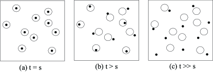
Figure 2: Sketch (two-dimensional cross section) of vortex line elements (small solid dots) and the associated circles with radius $\alpha b_{0}$ (large open circles) at different observation times.Thananart (a) At $t=s$, each vortex line element by construction resides inside its own circle and gives a count $\sum_{i}n_{i}(t=s)=N_{S}$ ($=10$ here). (b) At later times $t>s$, the repulsive vortex interactions cause the flux line elements to move away from their initial positions. This results in a smaller occupation number $\sum_{i}n_{i}(t>s)<N_{S}$ ($=5$ in this example). (c) At long times $t\gg s$, it is possible that all vortex line elements have left the circle, $n_{i}(t\gg s)=0$, which results in a complete decorrelation. For instance, the quantity $\sum_{i}n_{i}(s)n_{i}(t)$ in the pictures at these three times is evaluated to be $10$ at $t=s$, $5$ at $t>s$, and $0$ for $t\gg s$.

III Relaxation processes

In order to fully understand the non-equilibrium relaxation processes and aging phenomena in disordered type-II superconductors at low temperatures, we found it imperative to carefully disentagle the dynamical contributions originating from the repulsive interactions between the vortex lines and from their pinning to attractive point defects. We start our discussion with free flux lines, mainly in order to validate our code by comparing our data with the theoretically expected behavior and earlier work. We will then separately consider the effects of attractive point pins and of the long-range repulsive vortex interactions, before we at last venture to study the interplay of these two competing mechanisms to induce or relax correlations in the system.

III.1 Free elastic line

The relaxation kinetics of a single free elastic vortex line constitutes a valuable benchmark to check our program as this case can be easily understood by recalling that in the presence of thermal noise a fluctuating interface that tries to minimize its line tension should be described in the continuum limit by the linear Edwards–Wilkinson equation.Edw82 As the fluctuations in the transverse $x$ and $y$ directions are independent random variables for our free line, we expect the results for the free vortex to be described by the one-dimensional version of that well-known stochastic equation ($h$ below stands for either $x$ or $y$):

$$\frac{\partial h(z,t)}{\partial t}=\nu\,\partial_{z}^{2}h(z,t)+\eta(z,t)\ ,$$ (6)

where $\eta(z,t)$ represents a Gaussian white noise with zero mean and covariance $\langle\eta(z,t)\eta(z^{\prime},t^{\prime})\rangle=\frac{2T}{\nu}\delta(t-t^{\prime})\delta(z-z^{\prime})$, $\nu$ is the line stiffness (equal to ${\tilde{\epsilon}_{1}}$ here), and $T$ the temperature of the heat bath. The Edwards–Wilkinson equation, as well as a range of microscopic models belonging to the same dynamic universality class, has been studied extensively. Starting from a straight line, one first observes a short-time regime with uncorrelated fluctuations, which is rapidly replaced by a correlated intermediate-time interval characterized by a non-trivial power law increase of the line roughness. After a crossover time that algebraically depends on the system size, this correlated regime finally reaches the steady-state or saturation regime.

Two-time quantities have also been studied in the context of the Edwards–Wilkinson equation,Rothlein ; BCI ; Chou10 , facilitated by the fact that a full analytical analysis is possible for the linear stochastic equation (6). For example, in the correlated regime of the one-dimensional Edwards–Wilkinson equation the following exact expression for the height-height autocorrelation function has been derived:Rothlein

$$C(t,s)=C_{0}s^{1/2}\left[\left(\frac{t}{s}+1\right)^{1/2}-\left(\frac{t}{s}-1\right)^{1/2}\right]\ ,$$ (7)

where $C_{0}$ is a known constant. The detailed crossover properties of two-time quantities in the region between the correlated and saturated regimes have been carefully investigated in Ref. [BCI, ].

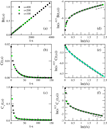
Figure 3: (Color online) Various two-time quantities for the free elastic vortex line obtained in systems with (a-c) $L=10$ and (d-f) $L=2560$ planes, and averaged over typically 200 independent Monte Carlo simulation runs; (a) and (d): mean-square displacement, (b) and (e): height-height autocorrelation function, (c) and (f): vortex density-density autocorrelation function (measured with $\alpha=0.05$). Data obtained for different waiting times are shown. For $L=10$ layers the system rapidly reaches the steady state, and time-translation invariance is recovered, i.e., the two-time quantities only depend on the time difference $t-s$. For $L=2560$ aging and dynamic scaling prevail throughout the simulation time window. The full line in (e) indicates the exact expression (7) derived from the Edwards–Wilkinson equation. The dashed lines in (d) and (f) indicate the predicted asymptotic power laws with exponents $1/2$ and $-1/2$, respectively. Here and in the following figures error bars are much smaller than the symbol sizes.

In Fig. 3, we display our Monte Carlo simulation results for our elastic vortex line model when both the vortex interaction and the defect pinning are switched off, i.e., only the first contribution in (1) is retained. One immediately notices a striking difference between the behavior of a “thin film” composed of only a few layers (such as $L=10$, see Figs. 3a–3c) and “bulk” systems consisting of many layers ($L=2560$, see Figs. 3d–3f). In the former case, the system rapidly evolves into the steady-state regime, yielding two-time quantities that only depend on the elapsed time difference $t-s$. As a result, the transverse displacements in the $x$ and $y$ directions perform simple random walks, as is revealed by the linear increase of the mean-square displacement with time, see Fig. 3a. For the larger bulk system, the correlated regime persists throughout the duration of our simulations, and both waiting and observation times reside well within that extended intermediate regime. This gives rise to aging and dynamical scaling: Time-translation invariance is broken, and all the two-time quantities display full-aging scaling.Henkel09 For each two-time observable we find the following scaling behavior (here given for the height autocorrelation function $C(t,s)$):

$$C(t,s)=s^{-b}f_{C}(t/s)\ ,$$ (8)

where $b$ represents an aging scaling exponent and $f_{C}(y)$ denotes an associated scaling function that follows a power law decay for large arguments. For the height-height autocorrelation we have $b=-1/2$.Rothlein In Fig. 3e we explicitly compare our numerically determined scaling function with the expression (7) resulting from the direct solution of the Edwards–Wilkinson equation (full line), and obtain perfect agreement.

Summarizing, we see that the free vortex line fluctuations are indeed aptly described by the one-dimensional Edwards–Wilkinson equation (6). We also observe a strong dependence on the system’s extension $L$ in the magnetic field direction, i.e., the vortex length: On the time scale of our simulations, the stationary regime is almost immediately reached when the system consists of only a few layers; in contrast, for larger bulk systems aging and dynamical scaling are observed easily. This points to quite distinct relaxation behavior in thin superconducting films and thicker bulk samples. We decided to avoid the additional complications stemming from the crossover between the correlated and steady-state regimes in our present study, and to rather focus on system sizes sufficiently large that no finite-size effects (no crossover to the steady state) are observed on the accessed time scales. Properties of smaller systems and possible experimental consequences for thin superconducting films will be discussed in a separate publication.

III.2 Pinning without interactions

Intuitively, one anticipates pinning centers to strongly influence the thermal fluctuations of our elastic flux lines. Indeed, attractive forces emanating from the pinning centers will tend to localize vortex segments, and thus ultimately suppress thermal fluctuations. Depending on the pinning strength, flux line elements will end up spending an appreciable amount of time close to a pinning center. Therefore, compared to freely fluctuating lines, a marked increase of correlations as function of time must be expected.

Before we proceed to analyze the influence of pinning centers in more detail, we need to stress that we exclusively consider attractive point defects, in accordance with the physics of disordered type-II superconductors in the low-temperature regime. A recent study [IBKC, ] addressed the relaxation and aging properties of elastic lines subjected to a random potential, corresponding to both attractive and repulsive pinning centers. Whereas a Gaussian disorder strength distribution certainly is a good model for disordered ferromagnets, its relevance for relaxation processes in disordered type-II superconductors at low temperatures is less obvious.

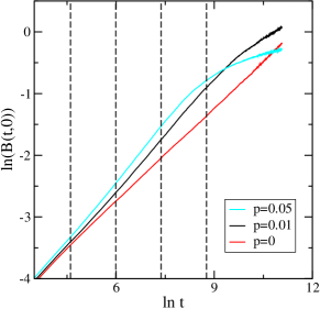
Figure 4: (Color online) Mean-square displacement $B(t,0)$ vs. time $t$ (in MCS) for different values of the pinning strength $p$, for systems of size $L=640$. In the initial time regime, the pinning centers attract the vortex segments as revealed by an increase of the slope of $B(t,0)$ as compared to a pure system. At later times the localization of the flux line elements induced by the pinning yields a strong decrease of this slope. The data shown result from averaging over typically 100 independent runs. The dashed lines indicate the times $t=100$, $400$, $1600$, and $6400$ MCS, see Fig. 5 below.

Let us start by looking at the mean-square displacement $B(t,0)$, with $s=0$, which gives a measure of the (squared) distance traveled by the flux line elements since the initial preparation of the system. In Fig. 4 we compare the behavior of a free elastic line with that of flux lines subject to pinning centers of various strengths $p=U_{0}/\epsilon_{0}$. The presence of attractive pins clearly gives rise to different regimes. The flux lines are rapidly attracted by the point defects, which yields an increase of the slope in the log-log plots of $B(t,0)$ vs. time $t$. This continues until some pinning strength-dependent crossover time at which the slope decreases even below the value of the free line, signifying the confinement of localized vortex segments to the vicinity of the pins. As one would expect, this crossover time decreases for increasing pinning strengths. For $p\geq 0.05$, $B(t,0)$ remains essentially unchanged, which indicates that for non-interacting lines there exists a critical pinning strength above which thermal fluctuations are no longer sufficiently strong to allow the vortex line elements to escape from the defects.

These different regimes also manifest themselves when two-time quantities are considered, as seen in Fig. 5, where we have plotted the data according to the free-line scaling behavior. Of course, it is not to be expected that these scaling laws remain valid when attractive defects are added to the system, but this representation of our data facilitates the following discussion. We first remark, see Figs. 5a and 5d, that the change of the slope of $B(t,0)$ translates into deviations of the mean-square displacement $B(t,s)$ from the free-line scaling that can be readily understood. For example, for $p=0.01$ the time intervals $[25,250]$, $[100,1000]$, and $[400,4000]$, used to compute $B(t,s)$ for the waiting times $s=25$, $100$, and $400$, respectively, correspond to the time regime with increasing local slopes of $B(t,0)$, compare Fig. 4. This yields a shift of $\ln(s^{-0.5}B(t,s))$ to higher values. As the crossover time of $B(t,0)$ lies inside the interval $[1600,16000]$, the converse behavior is observed for $s=1600$ and even larger waiting times, with a shift of $\ln(s^{-0.5}B(t,s))$ to lower values. This effect is more pronounced for larger pinning strengths, since then the crossover of $B(t,0)$ takes place earlier.

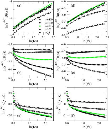
Figure 5: (Color online) Various two-time quantities for non-interacting vortex lines subject to attractive point defects of strengths (a-c) $p=0.01$ and (d-f) $p=0.05$: (a) and (d) mean-square displacement; (b) and (e) height-height autocorrelation function; (c) and (f) vortex density-density autocorrelation (with $\alpha=0.05$). The shown data result from averaging over typically 100 independent runs in systems of size $L=640$. For direct comparison with Fig. 3, the data are plotted according to the scaling properties of free elastic lines. Whereas an approximate scaling prevails for small waiting times (especially for the mean-square displacement and the vortex density-density autocorrelation), strong deviations emerge for larger waiting times. In (e) the apparent collapse of the height autocorrelation function for the largest waiting times is merely caused by the scale used in that figure.

The strongest influence of point defects and largest deviations from free elastic lines are observed in the height autocorrelation function, Figs. 5b and 5e. As the flux line elements are trapped by the pinning centers, their transverse in-plane displacements become diminished, which leads to an increase of the correlations as a function of waiting time. In addition, the decay of $C(t,s)$ as a function of $t$ is much slower for larger values of $s$. For larger pinning strengths and long waiting times we even observe non-monotonic temporal evolution, as the trapped flux lines experience an increase of the height correlations.

Finally, the vortex density-density autocorrelation turns out to be the least sensitive among our two-time observables to the presence of pinning centers, at least for comparatively small waiting times, see Figs. 5c and 5f. Indeed, for moderate values of $s$ one still observes the free-line scaling behavior; this is of course a consequence of our prescription for the computation of this correlation function, namely setting a circular area with fixed radius around every vortex line element at time $s$: As long as only a few line elements are captured by a point defect, the scaling of $C_{v}(t,s)$ remains approximately unchanged. Only when the majority of the vortex segments become trapped, does this localization induce a strong enhancement of the vortex density-density correlations.

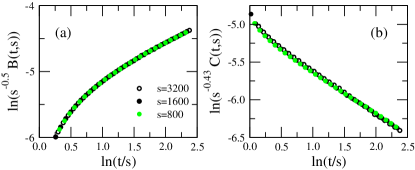
Figure 6: (Color online) (a) Mean-square displacement and (b) height-height autocorrelation function for non-interacting vortex lines subject to both attractive and repulsive point defects with strengths drawn from the square distribution $\left[-0.01,0.01\right]$. The shown data result from averaging over typically 100 independent runs in systems of size $L=1280$. The data display simple aging scaling, with different exponents for the two quantities.

To conclude this section, we note that the non-equilibrium relaxation physics is drastically different when both attractive and repulsive pinning centers are implemented. As studied in Ref. [IBKC, ] (see also Refs. [Noh09, ; Mon09, ]) an elastic line in a random potential is characterized by a time-dependent correlation length that crosses over from an early time power law growth to an asymptotic logarithmic growth. Consequently, two-time quantities display an apparent simple aging scaling with effective exponents that depend on temperature and on the randomness. We have verified that we obtain similar results as in Ref. [IBKC, ] when using both attractive and repulsive defects in our model and Monte Carlo algorithm. Indeed, as shown in Fig. 6, the time-dependent correlation length gives rise to simple aging scaling of our two-time quantities, with effective exponents that display a dependence on temperature and on the distribution of the pinning strengths. These crossover features also capture most of the relevant properties of disordered ferromagnets undergoing phase ordering.Par10 ; Cor10 ; Cor11 In Refs. [BCD1, ; BCD2, ], disordered type-II superconductors in the low-temperature phase were modeled by a corresponding model with random pins that are either attractive or repulsive. However, the physical realization relevant to materials is that of purely attractive pins, similar to those studied in our present work. Yet since the properties of elastic lines strongly depend on the nature of the pinning centers, any conclusions regarding the non-equilibrium relaxation properties of disordered type-II superconductors at low temperatures that are inferred from models with both attractive and repulsive defects should be viewed with some scepticism.

III.3 Interacting vortex lines without pinning

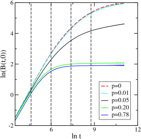
Figure 7: (Color online) Mean-square displacement $B(t,0)$ vs. time $t$ (in MCS) for interacting vortex lines with different values of the pinning strength $p$ (system size $L=640$; the data result from averaging over typically 100 independent runs). Due to the long-range interactions, the flux lines aim to maximize their separations, thus yielding values of $B(t,0)$ that are two orders of magnitude larger than in the absence of repulsive forces, compare Fig. 4. These displacements are impeded and vortex motion eventually stopped by the caging constraints of neighboring lines and pinning to attractive point defects. The (red) dashed line displays our data for a pure system, in the absence of pinning centers. The vertical dashed lines indicate the times $t=100$, $400$, $1600$, and $6400$ MCS.

In the absence of disorder our system composed of interacting flux lines evolves toward a regular triangular Abrikosov lattice. As we start our simulations by deposing initially straight lines at random positions, large displacements of the flux line elements are expected, as the system tries to minimize the long-range in-plane repulsive vortex interaction energy. The ensuing dynamic regimes are again nicely captured by the mean-square displacement $B(t,0)$ which takes on values that are two orders of magnitude larger than in the absence of interactions, see the (red) dashed line in Fig. 7. While the flux line segments experience these large displacements, $B(t,0)$ displays an approximate power law increase with time, with an effective exponent of $\approx 1.68$. Once the majority of vortices have reached the vicinity of their final equilibrium positions, the slope of $B(t,0)$ starts to gradually decrease.

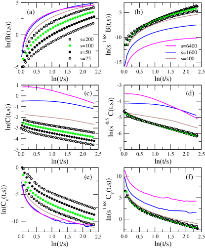
Figure 8: (Color online) Two-time quantities for interacting vortices in the absence of pinning centers: (a) and (b) mean-square displacement; (c) and (d) height-height autocorrelation function; (e) and (f) vortex density-density autocorrelation (with $\alpha=0.05$). Data obtained for different waiting times $s$ are shown, typically obtained from averaging over 500 independent simulation runs; the system size is $L=640$. (a), (c), and (e) display the unscaled data in a log-log plot, whereas (b), (d), and (f) show the approximate scaling observed for not too large waiting times. This scaling regime corresponds to the intermediate time window where $B(t,0)$ exhibits a power law increase as a function of time, with an (effective) exponent $\approx 1.68$, see Fig. 7.

The two-time quantities reveal both the initial-time regime as well as the crossover at later times, see Fig. 8. The mean-square displacement $B(t,s)$ yields a reasonably good data collapse for the smaller waiting times with the scaling exponent $-1.68$ that follows from the slope of $B(t,0)$ in that regime. When the observation time $t$ exceeds the crossover time, this scaling breaks down. Instead the growth rate of $B(t,s)$ decreases strongly with increasing $s$, even resulting in a crossing of the curves for different waiting times. The behavior of $B(t,s)$ is mirrored by that of the vortex density autocorrelation function: For small waiting times $s$, scaling is achieved with exponent $1.68$, whereas for larger waiting times the decay of the correlation slows down as $s$ increases. From these results we infer that the vortex density-density autocorrelation contains essentially the same physical information as the mean-square displacement. Interestingly, the height-height autocorrelation function displays a different scaling for smaller waiting times, given by the scaling exponent $b=-0.5$ of the free line, see Figs. 8c and 8d. This means that during the initial rearrangement of the vortex lines the height fluctuations are essentially the same as for the free line. Only when the vortices come close to their equilibrium positions does the character of the correlations change, reflecting the presence of long-range repulsive forces.

III.4 Interacting vortex lines with pinning

We are now ready to study the combined effects of repulsive flux line interactions and point defect pinning during the non-equilibrium relaxation of vortex matter in disordered type-II superconductors. We again begin by first considering the mean-square displacement $B(t,0)$, see Fig. 7. Adding very weak attractive defects, e.g., with $p=0.01$, has only a very minor effect on the time evolution of $B(t,0)$. Strengthening the point pins leads to a smaller rate of increase for the mean-square displacement, see the curve for $p=0.05$. At early times the flux lines are still displaced from their initial positions, as the vortex interactions try to establish an Abrikosov lattice. However, at intermediate times these displacements are impeded by the defects that noticeably slow down vortex motion. As a result the system tends to a new (quasi-)equilibrium state that balances these two competing mechanisms. For even stronger pinning, the moving flux lines become rapidly trapped by the disorder and the system gradually freezes into a blocked configuration. In Fig. 7 this is clearly the case for both $p=0.20$ and $p=0.78$.

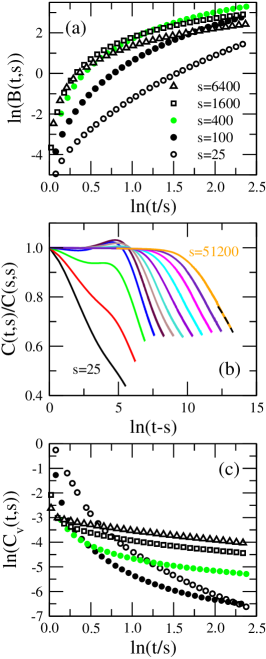
Figure 9: (Color online) Two-time quantities for interacting vortices in the presence of attractive pinning centers: (a) mean-square displacement; (b) height-height autocorrelation function; and (c) vortex density-density autocorrelation (with $\alpha=0.05$). The pinning strength here is $p=0.05$, the system size $L=640$, and the data result from averaging over typically 800 independent simulation runs. The waiting times $s$ for the vortex density autocorrelation are the same as those for the mean-square displacement. For the height autocorrelation function, the waiting times range from $s=25$ to $s=51200$, the values of $s$ being doubled between consecutive curves. The (normalized) height-height autocorrelation function, after a crossover, displays the same qualitative behavior as that encountered in structural glasses. For large values of $t-s$, the height autocorrelation assumes the stretched exponential form (9) with $\beta=0.4$, as shown by the dashed line overlying the $s=51200$ data.

The most interesting scenario naturally emerges for intermediate defect strengths. Indeed, when the pins are very weak, the rearrangement of the flux lines is barely affected, and all studied two-time quantities quantitatively display the same behavior as in a pure system. On the other hand, when the defects are too strong, the flux line elements remain firmly attached to the pinning centers, and a frozen configuration ensues. The non-trivial behavior at intermediate pinning strengths is studied in more detail in Fig. 9 for the case $p=0.05$.

The data for $B(t,s)$ and $C_{v}(t,s)$ shown in Figs. 9a and 9c are readily understood by comparing them to the corresponding results for the pure case, see Figs. 8a and 8e. The difference between these data sets is the absence of the early-time regime where $B(t,0)$ has an approximately constant slope, see Fig. 7. Consequently the data with $p=0.05$ do not allow any data collapse, not even for the smallest waiting times considered. However, this is the only noticeable difference, and the behavior for larger waiting times is qualitatively the same as for $p=0$, except that the decrease in slope of $B(t,s)$ for larger values of $s$ is stronger when $p\neq 0$.

However, a completely different picture emerges for the evolution of the normalized height-height autocorrelation function. As shown in Fig. 9b, for waiting times $s$ larger than a certain crossover value, $C(t,s)$ exhibits the typical two-step relaxation of a structural glass: An initial time-translation invariant regime, which corresponds to the so-called $\beta$ relaxation in glasses and only depends on the elapsed time difference $t-s$, is followed by a slow decay that is usually referred to as $\alpha$ relaxation in the glass literature.Gotze In the long-time limit we can fit this slow decay to a stretched exponential

$$f(\tau)=\exp\left[-\left(\frac{\tau}{t_{d}(s)}\right)^{\beta}\right]\ ,$$ (9)

with $\tau=t-s$, and a waiting-time dependent decorrelation time $t_{d}(s)$. For our different waiting times we obtain a consistent value $\beta\approx 0.40$ for the stretching exponent in Eq. (9). This emergence of a characteristic two-step glass-like relaxation is very intriguing. Obviously, the flux lines do not settle into a stable microstate even after their lateral displacements have become strongly reduced owing to the capture by the attractive pinning centers and the caging due to their repelling neighboring vortices. Instead, as a consequence of the two competing relaxation mechanisms, collective dynamics and slow decorrelation sets in that yields the typical two-step relaxation dynamics of a glass.

We also note the intriguing shape of the normalized height autocorrelation function in the crossover regime. Indeed, at intermediate waiting times $C(t,s)$ displays a strongly non-monotonic behavior, with a maximal value that even exceeds the value $C(s,s)$ at $t=s$. This remarkable feature points to a fundamental change in the nature of the emerging correlations, which is due to the trapping of vortex segments in the vicinity of the defects and the subsequent balancing of the competition between the attractive pinning and the repulsive interactions.

IV Discussion and conclusion

Our three-dimensional Monte Carlo investigation of relaxation processes in disordered type-II superconductors has allowed us to gain a thorough understanding of the non-equilibrium properties of these technologically important materials. We find the relaxation processes to be dominated by the interplay of two competing interactions, namely the pinning of the flux line elements to attractive point defects and the long-range mutual repulsion of the vortices. This competition generates various crossover scenarios that we have discussed systematically. The most interesting regime emerges for pinning centers of intermediate strength, for which we observe a distinguished two-step relaxation and a final slow, stretched-exponential decay of the height-height autocorrelation function. This behavior is reminiscent of that encountered in structural glasses, clearly demonstrating that disordered type-II superconductors subject to point defects indeed display pronounced glassy behavior at low temperatures, again justifying the term “vortex glass” for this frustrated pinned low-temperature phase.

We remark that our results are at variance with recent investigations based on three-dimensional London–Langevin dynamics simulations, where standard aging and dynamical scaling behavior of two-time quantities was observed,BCD1 ; BCD2 akin to the relaxation features of elastic lines in a random medium.IBKC However, these studies, in addition to difference in sample preparation, system size, and boundary conditions in the $z$-direction, employed a coarse-grained continuous random medium model of disordered type-II superconductors that becomes adequate near the normal- to superconducting transition, but does not realistically capture superconducting materials at low temperatures for which isolated defects such as oxygen vacancies always induce a local suppression of the transition temperature and therefore constitute attractive localized pinning centers for vortices. As our study shows, dynamical scaling no longer prevails for purely attractive point pinning centers, but instead much richer glassy relaxation dynamics sets in.

As already mentioned in the Introduction, it is essential for investigations of non-equilibrium systems to study different dynamics and their algorithmic implementations in order to ensure that any ensuing results indeed describe actual physical properties of the system rather than numerical artifacts. We have therefore recently begun to implement corresponding London–Langevin dynamics simulations for our elastic line model (1) with exclusively attractive pinning centers.Dob11 Our first tentative findings are in complete agreement with the Monte Carlo simulation results reported in this paper: They too show the emergence of glass-like behavior, with a slow, stretched-exponential decay at long times. An in-depth analysis of this dynamics is currently in progress; this comparative study also aims at matching the different microscopic time scales implicit in Monte Carlo and Langevin dynamical simulations.

Our current study can readily be expanded in various directions. Our results are valid in the regime where all time-dependent length scales remain small compared to the size of the system. However, many transport and relaxation experiments are carried out on thin superconducting films rather than bulk samples. In our model, a finite (small) number of layers introduces a dominant new length scale that substantially changes the relaxation processes, leading to additional crossover features. We also note that other types of defects can be experimentally realized, ranging from parallel and splayed columnar pins to planar defects, and combinations thereof with point disorder. It is an open and intriguing problem to understand how these different defect configurations influence the out-of-equilibrium relaxation processes in type-II superconductors. A detailed understanding of the relaxation phenomena in superconducting materials may facilitate characterization and optimization of samples with respect to pinning and flux transport. Finally, in all transport applications the flux lines are driven across the samples by external currents, which at long times yields a non-equilibrium steady state replacing the thermal equilibrium state that emerges without drive. Following similar lines as in the present study, one should be able to also analyze the relaxation properties of driven disordered type-II superconductors in a comprehensive manner. We plan to address these and related problems in the future.

- (1) L.C.E. Struik, Physical Aging in Amorphous Polymers and Other Materials (Elsevier, Amsterdam, 1978).
- (2) For recent overviews, see: M. Henkel, M. Pleimling, and R. Sanctuary (eds.), Ageing and the glass transition, Lecture Notes in Physics 716 (Springer, Berlin, 2007).
- (3) M. Henkel and M. Pleimling, Non-Equilibrium Phase Transitions, Volume 2: Ageing and Dynamical Scaling Far From Equilibrium (Springer, 2010).
- (4) L.F. Cugliandolo, in: Slow Relaxation and Non Equilibrium Dynamics in Condensed Matter, eds. J.-L. Barrat, J. Dalibard, J. Kurchan, and M.V. Feigel’man (Springer, 2003).
- (5) M. Henkel and M. Pleimling, in Rugged Free Energy Landscapes: Common Computational Approaches in Spin Glasses, Structural Glasses and Biological Macromolecules, ed. W. Janke, Lecture Notes in Physics 736, 107 (Springer, 2008).
- (6) For a now classical general review, see: G. Blatter, M.V. Feigel’man, V.B. Geshkenbein, A.I. Larkin, and V.M. Vinokur, Rev. Mod. Phys. 66, 1125 (1994).
- (7) S.S. Banerjee et al., Physica C 355, 39 (2001).
- (8) D.R. Nelson, Phys. Rev. Lett. 60, 1973 (1988); D.R. Nelson and H.S. Seung, Phys. Rev. B 39, 9153 (1989); D.R. Nelson, J. Stat. Phys. 57, 511 (1989).
- (9) M.P.A. Fisher, Phys. Rev. Lett. 62, 1415 (1989); D.S. Fisher, M.P.A. Fisher, and D.A. Huse, Phys. Rev. B 43, 130 (1991).
- (10) M.V. Feigel’man, V.B. Geshkenbein, A.I. Larkin, and V.M. Vinokur, Phys. Rev. Lett. 63, 2303 (1989).
- (11) T. Nattermann, Phys. Rev. Lett. 64, 2454 (1990).
- (12) For clear structural experimental evidence, see: U. Divakar et al., Phys. Rev. Lett. 92, 237004 (2004).
- (13) T. Giamarchi and P. Le Doussal, Phys. Rev. Lett. 72, 1530 (1994); Phys. Rev. B 52, 1242 (1995); Phys. Rev. Lett. 76, 3408 (1996); Phys. Rev. B 55, 6577 (1997); T. Klein, I. Joumard, S. Blanchard, J. Marcus, R. Cubitt, T. Giamarchi, and P. Le Doussal, Nature 413, 404 (2001).
- (14) J. Kierfeld, T. Nattermann, and T. Hwa, Phys. Rev. B 55, 626 (1997).
- (15) D.S. Fisher, Phys. Rev. Lett. 78, 1964 (1997).
- (16) G.I. Menon, Phys. Rev. B 65, 104527 (2002).
- (17) X. Du, G. Li, E.Y. Andrei, M. Greenblatt, and P. Shuk, Nature Physics 3, 111 (2007).
- (18) W. Henderson, E.Y. Andrei, M.J. Higgins, and S. Bhattacharya, Phys. Rev. Lett. 77, 2077 (1996).
- (19) M. Nicodemi and H.J. Jensen, Phys. Rev. Lett. 86, 4378 (2001); J. Phys. A: Math. Gen. 34, L11 (2001); Europhys. Lett. 54, 566 (2001); J. Phys. A: Math. Gen. 34, 8425 (2001); Phys. Rev. B 65, 144517 (2002).
- (20) C.J. Olson, C. Reichhardt, R.T. Scalettar, G.T. Zimanyi, and N. Grønbach-Jensen, Phys. Rev. B 67, 184523 (2003).
- (21) S. Bustingorry, L.F. Cugliandolo, and D. Domínguez, Phys. Rev. Lett. 96, 027001 (2006).
- (22) S. Bustingorry, L.F. Cugliandolo, and D. Domínguez, Phys. Rev. B 75, 024506 (2007).
- (23) S. Bustingorry, L.F. Cugliandolo, and J.L. Iguain, J. Stat. Mech. (2007) P09008.
- (24) J.L. Iguain, S. Bustingorry, A.B. Kolton, and L.F. Cugliandolo, Phys. Rev. B 80, 094201 (2009).
- (25) F. Romá and D. Domínguez, Phys. Rev. B 78, 184431 (2008).
- (26) A. van Otterlo, R.T. Scalettar, and G.T. Zimányi, Phys. Rev. Lett. 81, 1497 (1998).
- (27) D.R. Nelson and V.M. Vinokur, Phys. Rev. B 48, 13 060 (1993).
- (28) P. Sen, N. Trivedi, and D.M. Ceperley, Phys. Rev. Lett. 86, 4092 (2001).
- (29) A. Rosso and W. Krauth, Phys. Rev. B 65, 012202 (2001)
- (30) S. Tyagi and Y.Y. Goldschmidt, Phys. Rev. B 67, 214501 (2003).
- (31) V. Petäjä, M. Alava, and H. Rieger, Europhys. Lett. 66, 778 (2004).
- (32) J. Das, T.J. Bullard, and U.C. Täuber, Physica A 318, 48 (2003); T.J. Bullard, J. Das, G.L. Daquila, and U.C. Täuber, Eur. Phys. J. B 65, 469 (2008).
- (33) T. Klongcheongsan, Ph.D. thesis, Virginia Tech (2009); T. Klongcheongsan, T.J. Bullard, and U.C. Täuber, Supercond. Sci. Technol. 23, 025023 (2010).
- (34) A. Röthlein, F. Baumann, and M. Pleimling, Phys. Rev. E 74, 061604 (2006); Phys. Rev. E 76, 019901(E) (2007).
- (35) S. Bustingorry, J. Stat. Mech. (2007) P10002.
- (36) Y-L. Chou and M. Pleimling, J. Stat. Mech. (2010) P08007.
- (37) S.F. Edwards and D.R. Wilkinson, Proc. R. Soc. London Ser. A 381, 17 (1982).
- (38) J.D. Noh and H. Park, Phys. Rev. E 80, 040102(R) (2009).
- (39) C. Monthus and T. Garel, J. Stat. Mech. (2009) P12017.
- (40) H. Park and M. Pleimling, Phys. Rev. B 82, 144406 (2010).
- (41) F. Corberi, L.F. Cugliandolo, and H. Yoshino, Preprint arXiv:1010.0149.
- (42) F. Corberi, E. Lippiello, A. Mukherjee, S. Puri, and M. Zannetti, J. Stat. Mech. (2011) P03016.
- (43) W. Götze and L. Sjogren, Rep. Prog. Phys. 55, 241 (1992).
- (44) U. Dobramysl, M. Pleimling, and U.C. Täuber (work in progress).