A model of driven and decaying magnetic turbulence in a cylinder

Abstract

Using mean-field theory, we compute the evolution of the magnetic field in a cylinder with outer perfectly conducting boundaries, an imposed axial magnetic and electric field. The thus injected magnetic helicity in the system can be redistributed by magnetic helicity fluxes down the gradient of the local current helicity of the small-scale magnetic field. A weak reversal of the axial magnetic field is found to be a consequence of the magnetic helicity flux in the system. Such fluxes are known to alleviate so-called catastrophic quenching of the $\alpha$ effect in astrophysical applications. Application to the reversed field pinch in plasma confinement devices is discussed.

I Introduction

The interaction between a conducting medium moving at speed $\textstyle U$ through a magnetic field $\textstyle B$ is generally referred to as a dynamo effect. This effect plays important roles in astrophysics (Mof78, ; KR80, ), magnetospheric physics (Ogino, ), as well as laboratory plasma physics (Ji_etal96, ). It modifies the electric field in the rest frame, so that Ohm’s law takes the form $\mathchoice{\mbox{\boldmath$\displaystyle J$}}{\mbox{\boldmath$\textstyle J$}}{\mbox{\boldmath$\scriptstyle J$}}{\mbox{\boldmath$\scriptscriptstyle J$}}{}=\sigma\left(\mathchoice{\mbox{\boldmath$\displaystyle E$}}{\mbox{\boldmath$\textstyle E$}}{\mbox{\boldmath$\scriptstyle E$}}{\mbox{\boldmath$\scriptscriptstyle E$}}{}+\mathchoice{\mbox{\boldmath$\displaystyle U$}}{\mbox{\boldmath$\textstyle U$}}{\mbox{\boldmath$\scriptstyle U$}}{\mbox{\boldmath$\scriptscriptstyle U$}}{}\times\mathchoice{\mbox{\boldmath$\displaystyle B$}}{\mbox{\boldmath$\textstyle B$}}{\mbox{\boldmath$\scriptstyle B$}}{\mbox{\boldmath$\scriptscriptstyle B$}}{}\right)$, where $\textstyle J$ is the current density, $\textstyle E$ is the electric field, and $\sigma$ is the conductivity. Of particular interest for the present paper is the case where an external electric field $\mathchoice{\mbox{\boldmath$\displaystyle E$}}{\mbox{\boldmath$\textstyle E$}}{\mbox{\boldmath$\scriptstyle E$}}{\mbox{\boldmath$\scriptscriptstyle E$}}{}^{\rm ext}$ is induced through a transformer with a time-varying magnetic field, as is the case in many plasma confinement experiments. With the external electric field included, Ohm’s law becomes

$$\mathchoice{\mbox{\boldmath$\displaystyle J$}}{\mbox{\boldmath$\textstyle J$}}{\mbox{\boldmath$\scriptstyle J$}}{\mbox{\boldmath$\scriptscriptstyle J$}}{}=\sigma\left(\mathchoice{\mbox{\boldmath$\displaystyle E$}}{\mbox{\boldmath$\textstyle E$}}{\mbox{\boldmath$\scriptstyle E$}}{\mbox{\boldmath$\scriptscriptstyle E$}}{}+\mathchoice{\mbox{\boldmath$\displaystyle E$}}{\mbox{\boldmath$\textstyle E$}}{\mbox{\boldmath$\scriptstyle E$}}{\mbox{\boldmath$\scriptscriptstyle E$}}{}^{\rm ext}+\mathchoice{\mbox{\boldmath$\displaystyle U$}}{\mbox{\boldmath$\textstyle U$}}{\mbox{\boldmath$\scriptstyle U$}}{\mbox{\boldmath$\scriptscriptstyle U$}}{}\times\mathchoice{\mbox{\boldmath$\displaystyle B$}}{\mbox{\boldmath$\textstyle B$}}{\mbox{\boldmath$\scriptstyle B$}}{\mbox{\boldmath$\scriptscriptstyle B$}}{}\right).$$ (1)

In a turbulent medium, often only averaged quantities (indicated below by overbars) are accessible. The averaged form of Ohm’s law reads

$$\overline{\mbox{\boldmath$J$}}=\sigma\left(\overline{\bm{E}}+\overline{\bm{E}}^{\rm ext}+\overline{\bm{U}}\times\overline{\bm{B}}+\overline{\mbox{\boldmath${\cal E}$}}{}\right),$$ (2)

where $\overline{\mbox{\boldmath${\cal E}$}}{}=\overline{\mathchoice{\mbox{\boldmath$\displaystyle u$}}{\mbox{\boldmath$\textstyle u$}}{\mbox{\boldmath$\scriptstyle u$}}{\mbox{\boldmath$\scriptscriptstyle u$}}{}\times\mathchoice{\mbox{\boldmath$\displaystyle b$}}{\mbox{\boldmath$\textstyle b$}}{\mbox{\boldmath$\scriptstyle b$}}{\mbox{\boldmath$\scriptscriptstyle b$}}{}}$ is referred to as the mean $\overline{\mbox{\boldmath${\cal E}$}}{}=\overline{\mathchoice{\mbox{\boldmath$\displaystyle u$}}{\mbox{\boldmath$\textstyle u$}}{\mbox{\boldmath$\scriptstyle u$}}{\mbox{\boldmath$\scriptscriptstyle u$}}{}\times\mathchoice{\mbox{\boldmath$\displaystyle b$}}{\mbox{\boldmath$\textstyle b$}}{\mbox{\boldmath$\scriptstyle b$}}{\mbox{\boldmath$\scriptscriptstyle b$}}{}}$ is referred to as the mean turbulent electromotive force, and $\mathchoice{\mbox{\boldmath$\displaystyle u$}}{\mbox{\boldmath$\textstyle u$}}{\mbox{\boldmath$\scriptstyle u$}}{\mbox{\boldmath$\scriptscriptstyle u$}}{}=\mathchoice{\mbox{\boldmath$\displaystyle U$}}{\mbox{\boldmath$\textstyle U$}}{\mbox{\boldmath$\scriptstyle U$}}{\mbox{\boldmath$\scriptscriptstyle U$}}{}-\overline{\bm{U}}$ and $\mathchoice{\mbox{\boldmath$\displaystyle b$}}{\mbox{\boldmath$\textstyle b$}}{\mbox{\boldmath$\scriptstyle b$}}{\mbox{\boldmath$\scriptscriptstyle b$}}{}=\mathchoice{\mbox{\boldmath$\displaystyle B$}}{\mbox{\boldmath$\textstyle B$}}{\mbox{\boldmath$\scriptstyle B$}}{\mbox{\boldmath$\scriptscriptstyle B$}}{}-\overline{\bm{B}}$ are fluctuations of velocity and magnetic field, respectively. It has been known for some time that the averaged profiles, $\overline{\mbox{\boldmath$J$}}$ and $\sigma\overline{\bm{E}}^{\rm ext}$ do not agree in actual experiments. This disagreement cannot be explained by the $\overline{\bm{U}}\times\overline{\bm{B}}$ term either, leaving therefore $\overline{\mbox{\boldmath${\cal E}$}}{}$ as the only remaining term. Examples include the recent dynamo experiment in Cadarache Cadarache and in particular the reversed field pinch (RFP) BN80 ; Tay86 ; Ji_etal96 , which is one of the configurations studied in connection with fusion plasmas. The name of this device derives from the fact that the toroidal (or axial, in a cylindrical geometry) magnetic field reverses sign near the periphery. Indeed, in the astrophysical context it is well-known that the $\overline{\mbox{\boldmath${\cal E}$}}{}$ is responsible for the amplification and maintenance of large-scale magnetic fields (Mof78, ; KR80, ).

The analogy among the various examples of the $\overline{\mbox{\boldmath${\cal E}$}}{}$ term has motivated comparative research between astrophysics and plasma physics applications BJ06 . In these cases, $\overline{\mbox{\boldmath${\cal E}$}}{}$ is found to have a component proportional to the mean field ($\alpha\overline{\bm{B}}$, referred to as the $\alpha$ effect) and a component proportional to the mean current density ($\eta_{\rm t}\overline{\mbox{\boldmath$J$}}$, where $\eta_{\rm t}$ is the turbulent diffusivity). Since $\alpha$ is a pseudoscalar, one expects it to depend on the helicity of the flow, which is also a pseudoscalar. Decisive in developing the analogy between the $\alpha$ effects in astrophysics and laboratory plasma physics is the realization that $\alpha$ is caused not only by helicity in the flow (kinetic $\alpha$ effect), but also by that of the magnetic field itself PFL76 . This magnetic contribution to the $\alpha$ effect has received increased astrophysical interest, because there are strong indications that such dynamos saturate by building up small-scale helical fields that lead to a magnetic $\alpha$ effect which, in turn, counteracts the kinetic $\alpha$ effect FB02 ; BB02 ; Sub02 . This process can be described quantitatively by taking magnetic helicity evolution into account, which leads to what is known as the dynamical quenching formalism that goes back to early work of Kleeorin & Ruzmaikin KR82 . However, it is now also believed that such quenching would lead to a catastrophically low saturation field strength BS05 , unless there are magnetic helicity fluxes out of the domain that would limit the excessive build-up of small-scale helical fields BS04 . This would reduce the magnetic $\alpha$ effect and thus allow the production of mean fields whose energy density is comparable to that of the kinetic energy of the turbulence B05 .

These recent developments are purely theoretical, so the hope is that more can be learnt by applying the recently gained knowledge to experiments like the RFP BN80 ; Tay86 . Unlike tokamaks, the RFP is a relatively slender torus, so it makes sense to study its properties in a local model where one ignores curvature effects and considers a cylindrical piece of the torus. Along the axis of this cylinder there is a field-aligned current that makes the field helical. This field is susceptible to kink and tearing instabilities that lead to turbulence. It is generally believed that the resulting mean turbulent electromotive force $\overline{\mbox{\boldmath${\cal E}$}}{}$ is responsible for the field reversal Ji_etal96 ; JP02 . The turbulence is also believed to help driving the system toward a minimum energy state Tay74 . This state is nearly force-free and maintained by $\overline{\bm{E}}^{\rm ext}$. This adds to the notion that the RFP must be sustained by some kind of dynamo process AB84 . In Cartesian geometry such a slow-down has previously already been modeled using the dynamical quenching formalism YBR03 .

The RFP has been studied extensively using three-dimensional simulations AB84 ; SCN85 ; SMN96 ; CBE06 , which confirm the conjecture of J. B. Taylor Tay74 that the system approaches a minimum energy state. Additional understanding has been obtained using mean-field considerations Str85 ; BH86 . Both, here and in astrophysical dynamos there is an $\alpha$ effect that quantifies the correlation of the fluctuating parts of velocity and magnetic field. However, a major difference lies in the fact that in the RFP the $\alpha$ effect is caused by instabilities of the initially large-scale magnetic field while in the astrophysical case one is concerned with the problem of explaining the origin of large-scale fields by the $\alpha$ effect Mof78 ; KR80 . However, this distinction may be too simplistic and there is indeed evidence that in the RFP the $\alpha$ effect exists in close relation with a finite magnetic helicity flux Ji99 , supporting the idea that so-called catastrophic quenching is avoided by helicity transport.

The purpose of this paper is to apply modern mean-field dynamo theory with dynamical quenching to a cylindrical configuration to allow a more meaningful comparison between the $\alpha$ effect in astrophysics and the one occurring in RFP experiments.

II The model

To model the evolution of the magnetic field in a cylinder with imposed axial magnetic and electric fields, we employ mean-field theory, where the evolution of the mean field $\overline{\bm{B}}$ is governed by turbulent magnetic diffusivity and an $\alpha$ effect. Unlike the astrophysical case where $\alpha$ depends primarily on the kinetic helicity of the plasma, in turbulence from current-driven instabilities the $\alpha$ effect is likely to depend primarily on the current helicity of the small-scale field PFL76 . The current density is given by $\mathchoice{\mbox{\boldmath$\displaystyle J$}}{\mbox{\boldmath$\textstyle J$}}{\mbox{\boldmath$\scriptstyle J$}}{\mbox{\boldmath$\scriptscriptstyle J$}}{}=\mathchoice{\mbox{\boldmath$\displaystyle\nabla$}}{\mbox{\boldmath$\textstyle\nabla$}}{\mbox{\boldmath$\scriptstyle\nabla$}}{\mbox{\boldmath$\scriptscriptstyle\nabla$}}{}\times\mathchoice{\mbox{\boldmath$\displaystyle B$}}{\mbox{\boldmath$\textstyle B$}}{\mbox{\boldmath$\scriptstyle B$}}{\mbox{\boldmath$\scriptscriptstyle B$}}{}/\mu_{0}$, where $\mu_{0}$ is the vacuum permeability and $\mathchoice{\mbox{\boldmath$\displaystyle j$}}{\mbox{\boldmath$\textstyle j$}}{\mbox{\boldmath$\scriptstyle j$}}{\mbox{\boldmath$\scriptscriptstyle j$}}{}=\mathchoice{\mbox{\boldmath$\displaystyle\nabla$}}{\mbox{\boldmath$\textstyle\nabla$}}{\mbox{\boldmath$\scriptstyle\nabla$}}{\mbox{\boldmath$\scriptscriptstyle\nabla$}}{}\times\mathchoice{\mbox{\boldmath$\displaystyle b$}}{\mbox{\boldmath$\textstyle b$}}{\mbox{\boldmath$\scriptstyle b$}}{\mbox{\boldmath$\scriptscriptstyle b$}}{}/\mu_{0}$ is the fluctuating current density. The mean current helicity density of the small-scale field is then given by $\overline{\mathchoice{\mbox{\boldmath$\displaystyle j$}}{\mbox{\boldmath$\textstyle j$}}{\mbox{\boldmath$\scriptstyle j$}}{\mbox{\boldmath$\scriptscriptstyle j$}}{}\cdot\mathchoice{\mbox{\boldmath$\displaystyle b$}}{\mbox{\boldmath$\textstyle b$}}{\mbox{\boldmath$\scriptstyle b$}}{\mbox{\boldmath$\scriptscriptstyle b$}}{}}$. To a good approximation, the $\overline{\mathchoice{\mbox{\boldmath$\displaystyle j$}}{\mbox{\boldmath$\textstyle j$}}{\mbox{\boldmath$\scriptstyle j$}}{\mbox{\boldmath$\scriptscriptstyle j$}}{}\cdot\mathchoice{\mbox{\boldmath$\displaystyle b$}}{\mbox{\boldmath$\textstyle b$}}{\mbox{\boldmath$\scriptstyle b$}}{\mbox{\boldmath$\scriptscriptstyle b$}}{}}$ term is proportional to the small-scale magnetic helicity density, $\overline{\mathchoice{\mbox{\boldmath$\displaystyle a$}}{\mbox{\boldmath$\textstyle a$}}{\mbox{\boldmath$\scriptstyle a$}}{\mbox{\boldmath$\scriptscriptstyle a$}}{}\cdot\mathchoice{\mbox{\boldmath$\displaystyle b$}}{\mbox{\boldmath$\textstyle b$}}{\mbox{\boldmath$\scriptstyle b$}}{\mbox{\boldmath$\scriptscriptstyle b$}}{}}$, where $\mathchoice{\mbox{\boldmath$\displaystyle a$}}{\mbox{\boldmath$\textstyle a$}}{\mbox{\boldmath$\scriptstyle a$}}{\mbox{\boldmath$\scriptscriptstyle a$}}{}=\mathchoice{\mbox{\boldmath$\displaystyle A$}}{\mbox{\boldmath$\textstyle A$}}{\mbox{\boldmath$\scriptstyle A$}}{\mbox{\boldmath$\scriptscriptstyle A$}}{}-\overline{\mbox{\boldmath$A$}}$ is the vector potential of the fluctuating field. The generation of $\overline{\mathchoice{\mbox{\boldmath$\displaystyle a$}}{\mbox{\boldmath$\textstyle a$}}{\mbox{\boldmath$\scriptstyle a$}}{\mbox{\boldmath$\scriptscriptstyle a$}}{}\cdot\mathchoice{\mbox{\boldmath$\displaystyle b$}}{\mbox{\boldmath$\textstyle b$}}{\mbox{\boldmath$\scriptstyle b$}}{\mbox{\boldmath$\scriptscriptstyle b$}}{}}$ is coupled to the decay of $\overline{\mbox{\boldmath$A$}}\cdot\overline{\bm{B}}$ through the magnetic helicity evolution equation KR82 ; KRR95 ; FB02 ; BB02 such that $\overline{\mbox{\boldmath$A$}}\cdot\overline{\bm{B}}+\overline{\mathchoice{\mbox{\boldmath$\displaystyle a$}}{\mbox{\boldmath$\textstyle a$}}{\mbox{\boldmath$\scriptstyle a$}}{\mbox{\boldmath$\scriptscriptstyle a$}}{}\cdot\mathchoice{\mbox{\boldmath$\displaystyle b$}}{\mbox{\boldmath$\textstyle b$}}{\mbox{\boldmath$\scriptstyle b$}}{\mbox{\boldmath$\scriptscriptstyle b$}}{}}$ evolves only resistively in the absence of magnetic helicity fluxes.

Note that $\overline{\mathchoice{\mbox{\boldmath$\displaystyle a$}}{\mbox{\boldmath$\textstyle a$}}{\mbox{\boldmath$\scriptstyle a$}}{\mbox{\boldmath$\scriptscriptstyle a$}}{}\cdot\mathchoice{\mbox{\boldmath$\displaystyle b$}}{\mbox{\boldmath$\textstyle b$}}{\mbox{\boldmath$\scriptstyle b$}}{\mbox{\boldmath$\scriptscriptstyle b$}}{}}$ is in general gauge-dependent and might therefore not be a physically meaningful quantity. However, if there is sufficient scale separation, the mean magnetic helicity density of the fluctuating field can be expressed in terms of the density of field line linkages, which does not involve the magnetic vector potential and is therefore gauge-independent SB06 . For the large-scale field, on the other hand, the magnetic helicity density does remain in general gauge-dependent HB10 , but our final model will not be affected by this, because the magnetic helicity of the large-scale magnetic field does not enter in the mean-field model.

We model an induced electric field by an externally applied electric field $\mathchoice{\mbox{\boldmath$\displaystyle E$}}{\mbox{\boldmath$\textstyle E$}}{\mbox{\boldmath$\scriptstyle E$}}{\mbox{\boldmath$\scriptscriptstyle E$}}{}^{\rm ext}$. In the absence of any other induction effects this leads to a current density $\mathchoice{\mbox{\boldmath$\displaystyle J$}}{\mbox{\boldmath$\textstyle J$}}{\mbox{\boldmath$\scriptstyle J$}}{\mbox{\boldmath$\scriptscriptstyle J$}}{}=\sigma\mathchoice{\mbox{\boldmath$\displaystyle E$}}{\mbox{\boldmath$\textstyle E$}}{\mbox{\boldmath$\scriptstyle E$}}{\mbox{\boldmath$\scriptscriptstyle E$}}{}^{\rm ext}$. Furthermore, we ignore a mean flow ($\overline{\bm{U}}={\bf 0}$), and assume that the velocity field has only a turbulent component $\textstyle u$. For simplicity we assume that $\overline{\bm{E}}^{\rm ext}$ has no fluctuating part, i.e. $\mathchoice{\mbox{\boldmath$\displaystyle E$}}{\mbox{\boldmath$\textstyle E$}}{\mbox{\boldmath$\scriptstyle E$}}{\mbox{\boldmath$\scriptscriptstyle E$}}{}^{\rm ext}=\overline{\bm{E}}^{\rm ext}$. The decay of $\overline{\bm{B}}$ is accelerated by turbulent magnetic diffusivity $\eta_{\rm t}$, which is expected to occur as a result of the turbulence connected with kink and tearing instabilities inherent to the RFP. This mean turbulent electromotive force has two components corresponding to the $\alpha$ effect and turbulent diffusion with

$$\overline{\mbox{\boldmath${\cal E}$}}{}=\alpha\overline{\bm{B}}-\eta_{\rm t}\mu_{0}\overline{\mbox{\boldmath$J$}},$$ (3)

where we have ignored the fact that $\alpha$ effect and turbulent diffusion are really tensors. The evolution equation for $\overline{\bm{B}}$ is then given by the mean-field induction equation,

$${\partial\overline{\bm{B}}\over\partial t}=\mathchoice{\mbox{\boldmath$\displaystyle\nabla$}}{\mbox{\boldmath$\textstyle\nabla$}}{\mbox{\boldmath$\scriptstyle\nabla$}}{\mbox{\boldmath$\scriptscriptstyle\nabla$}}{}\times\left(\alpha\overline{\bm{B}}-\eta_{\rm T}\mu_{0}\overline{\mbox{\boldmath$J$}}+\overline{\bm{E}}^{\rm ext}\right),$$ (4)

where $\eta_{\rm T}=\eta_{\rm t}+\eta$ is the sum of turbulent and microscopic (Spitzer) magnetic diffusivities (not to be confused with the resistivity $\eta\mu_{0}$, which is also often called $\eta$). Note that only non-uniform and non-potential contributions to $\overline{\bm{E}}^{\rm ext}$ can have an effect.

As a starting point, we assume that the rms velocity $u_{\rm rms}$ and the typical wavenumber $k_{\rm f}$ of the turbulence are constant, although it is clear that these values should really depend on the level of the actual magnetic field. We estimate the value of $\eta_{\rm t}$ using a standard formula for isotropic turbulence,

$$\eta_{\rm t}={\textstyle{1\over 3}}\tau\overline{\mathchoice{\mbox{\boldmath$\displaystyle u$}}{\mbox{\boldmath$\textstyle u$}}{\mbox{\boldmath$\scriptstyle u$}}{\mbox{\boldmath$\scriptscriptstyle u$}}{}^{2}},$$ (5)

where $\tau=(u_{\rm rms}k_{\rm f})^{-1}$ is the correlation time of the turbulence and $u_{\rm rms}=(\overline{\mathchoice{\mbox{\boldmath$\displaystyle u$}}{\mbox{\boldmath$\textstyle u$}}{\mbox{\boldmath$\scriptstyle u$}}{\mbox{\boldmath$\scriptscriptstyle u$}}{}^{2}})^{1/2}$ is its rms velocity. Thus, we can also write $\eta_{\rm t}=u_{\rm rms}/3k_{\rm f}$. The turbulent velocity results from kink and tearing mode instabilities and will simply be treated as a constant in our model. For the $\alpha$ effect we assume that the kinetic helicity is negligible It would be much smaller than the current helicity, but of the same sign PFL76 , so it would contribute to quenching the $\alpha$ effect, and so we just take

$$\alpha={\textstyle{1\over 3}}\tau\overline{\mathchoice{\mbox{\boldmath$\displaystyle j$}}{\mbox{\boldmath$\textstyle j$}}{\mbox{\boldmath$\scriptstyle j$}}{\mbox{\boldmath$\scriptscriptstyle j$}}{}\cdot\mathchoice{\mbox{\boldmath$\displaystyle b$}}{\mbox{\boldmath$\textstyle b$}}{\mbox{\boldmath$\scriptstyle b$}}{\mbox{\boldmath$\scriptscriptstyle b$}}{}}/\rho_{0},$$ (6)

and use the fact that $\overline{\mathchoice{\mbox{\boldmath$\displaystyle j$}}{\mbox{\boldmath$\textstyle j$}}{\mbox{\boldmath$\scriptstyle j$}}{\mbox{\boldmath$\scriptscriptstyle j$}}{}\cdot\mathchoice{\mbox{\boldmath$\displaystyle b$}}{\mbox{\boldmath$\textstyle b$}}{\mbox{\boldmath$\scriptstyle b$}}{\mbox{\boldmath$\scriptscriptstyle b$}}{}}$ and $\overline{\mathchoice{\mbox{\boldmath$\displaystyle a$}}{\mbox{\boldmath$\textstyle a$}}{\mbox{\boldmath$\scriptstyle a$}}{\mbox{\boldmath$\scriptscriptstyle a$}}{}\cdot\mathchoice{\mbox{\boldmath$\displaystyle b$}}{\mbox{\boldmath$\textstyle b$}}{\mbox{\boldmath$\scriptstyle b$}}{\mbox{\boldmath$\scriptscriptstyle b$}}{}}$ are proportional to each other. Here, $\rho_{0}$ is the mean density of the plasma. For homogeneous turbulence we have $\overline{\mathchoice{\mbox{\boldmath$\displaystyle j$}}{\mbox{\boldmath$\textstyle j$}}{\mbox{\boldmath$\scriptstyle j$}}{\mbox{\boldmath$\scriptscriptstyle j$}}{}\cdot\mathchoice{\mbox{\boldmath$\displaystyle b$}}{\mbox{\boldmath$\textstyle b$}}{\mbox{\boldmath$\scriptstyle b$}}{\mbox{\boldmath$\scriptscriptstyle b$}}{}}=k_{\rm f}^{2}\overline{\mathchoice{\mbox{\boldmath$\displaystyle a$}}{\mbox{\boldmath$\textstyle a$}}{\mbox{\boldmath$\scriptstyle a$}}{\mbox{\boldmath$\scriptscriptstyle a$}}{}\cdot\mathchoice{\mbox{\boldmath$\displaystyle b$}}{\mbox{\boldmath$\textstyle b$}}{\mbox{\boldmath$\scriptstyle b$}}{\mbox{\boldmath$\scriptscriptstyle b$}}{}}/\mu_{0}$, although for inhomogeneous turbulence, $k_{\rm f}^{2}\overline{\mathchoice{\mbox{\boldmath$\displaystyle a$}}{\mbox{\boldmath$\textstyle a$}}{\mbox{\boldmath$\scriptstyle a$}}{\mbox{\boldmath$\scriptscriptstyle a$}}{}\cdot\mathchoice{\mbox{\boldmath$\displaystyle b$}}{\mbox{\boldmath$\textstyle b$}}{\mbox{\boldmath$\scriptstyle b$}}{\mbox{\boldmath$\scriptscriptstyle b$}}{}}/\mu_{0}$ has been found to be smaller than $\overline{\mathchoice{\mbox{\boldmath$\displaystyle j$}}{\mbox{\boldmath$\textstyle j$}}{\mbox{\boldmath$\scriptstyle j$}}{\mbox{\boldmath$\scriptscriptstyle j$}}{}\cdot\mathchoice{\mbox{\boldmath$\displaystyle b$}}{\mbox{\boldmath$\textstyle b$}}{\mbox{\boldmath$\scriptstyle b$}}{\mbox{\boldmath$\scriptscriptstyle b$}}{}}$ by a factor of two Mit10 . We compute the evolution of $\overline{\mathchoice{\mbox{\boldmath$\displaystyle a$}}{\mbox{\boldmath$\textstyle a$}}{\mbox{\boldmath$\scriptstyle a$}}{\mbox{\boldmath$\scriptscriptstyle a$}}{}\cdot\mathchoice{\mbox{\boldmath$\displaystyle b$}}{\mbox{\boldmath$\textstyle b$}}{\mbox{\boldmath$\scriptstyle b$}}{\mbox{\boldmath$\scriptscriptstyle b$}}{}}$ by considering first the evolution equation for $\overline{\mathchoice{\mbox{\boldmath$\displaystyle A$}}{\mbox{\boldmath$\textstyle A$}}{\mbox{\boldmath$\scriptstyle A$}}{\mbox{\boldmath$\scriptscriptstyle A$}}{}\cdot\mathchoice{\mbox{\boldmath$\displaystyle B$}}{\mbox{\boldmath$\textstyle B$}}{\mbox{\boldmath$\scriptstyle B$}}{\mbox{\boldmath$\scriptscriptstyle B$}}{}}$. Note that $\overline{\mathchoice{\mbox{\boldmath$\displaystyle A$}}{\mbox{\boldmath$\textstyle A$}}{\mbox{\boldmath$\scriptstyle A$}}{\mbox{\boldmath$\scriptscriptstyle A$}}{}\cdot\mathchoice{\mbox{\boldmath$\displaystyle B$}}{\mbox{\boldmath$\textstyle B$}}{\mbox{\boldmath$\scriptstyle B$}}{\mbox{\boldmath$\scriptscriptstyle B$}}{}}$ evolves only resistively, unless there is material motion through the domain boundaries HB10 , so we have

$${{\rm d}{}\over{\rm d}{}t}\overline{\mathchoice{\mbox{\boldmath$\displaystyle A$}}{\mbox{\boldmath$\textstyle A$}}{\mbox{\boldmath$\scriptstyle A$}}{\mbox{\boldmath$\scriptscriptstyle A$}}{}\cdot\mathchoice{\mbox{\boldmath$\displaystyle B$}}{\mbox{\boldmath$\textstyle B$}}{\mbox{\boldmath$\scriptstyle B$}}{\mbox{\boldmath$\scriptscriptstyle B$}}{}}=2\overline{\bm{E}}^{\rm ext}\cdot\overline{\bm{B}}-2\eta\mu_{0}\overline{\mathchoice{\mbox{\boldmath$\displaystyle J$}}{\mbox{\boldmath$\textstyle J$}}{\mbox{\boldmath$\scriptstyle J$}}{\mbox{\boldmath$\scriptscriptstyle J$}}{}\cdot\mathchoice{\mbox{\boldmath$\displaystyle B$}}{\mbox{\boldmath$\textstyle B$}}{\mbox{\boldmath$\scriptstyle B$}}{\mbox{\boldmath$\scriptscriptstyle B$}}{}}-\mathchoice{\mbox{\boldmath$\displaystyle\nabla$}}{\mbox{\boldmath$\textstyle\nabla$}}{\mbox{\boldmath$\scriptstyle\nabla$}}{\mbox{\boldmath$\scriptscriptstyle\nabla$}}{}\cdot\overline{\mbox{\boldmath${\cal F}$}}{},$$ (7)

where $\overline{\mbox{\boldmath${\cal F}$}}{}$ is the mean magnetic helicity flux. While $\overline{\bm{B}}$ evolves subject to the mean field equation (4), the magnetic helicity of the mean field will change subject to the equation

$${{\rm d}{}\over{\rm d}{}t}\left(\overline{\mbox{\boldmath$A$}}\cdot\overline{\bm{B}}\right)=2\overline{\mbox{\boldmath${\cal E}$}}{}^{\rm tot}\cdot\overline{\bm{B}}-2\eta\mu_{0}\overline{\mbox{\boldmath$J$}}\cdot\overline{\bm{B}}-\mathchoice{\mbox{\boldmath$\displaystyle\nabla$}}{\mbox{\boldmath$\textstyle\nabla$}}{\mbox{\boldmath$\scriptstyle\nabla$}}{\mbox{\boldmath$\scriptscriptstyle\nabla$}}{}\cdot\overline{\mbox{\boldmath${\cal F}$}}{}_{\rm m},$$ (8)

where $\overline{\mbox{\boldmath${\cal E}$}}{}^{\rm tot}=\overline{\mbox{\boldmath${\cal E}$}}{}+\overline{\bm{E}}^{\rm ext}$ and $\overline{\mbox{\boldmath${\cal F}$}}{}_{\rm m}=\overline{\bm{E}}\times\overline{\mbox{\boldmath$A$}}+\overline{\Phi}\,\overline{\bm{B}}$ is the mean magnetic helicity flux from the mean magnetic field, and $\overline{\Phi}$ is the mean electrostatic potential. Here, $\overline{\bm{E}}=\eta\mu_{0}\overline{\mbox{\boldmath$J$}}-\overline{\mbox{\boldmath${\cal E}$}}{}^{\rm tot}$ is the mean electric field. Subtracting (8) from (7), we find a similar evolution equation for $\overline{\mathchoice{\mbox{\boldmath$\displaystyle a$}}{\mbox{\boldmath$\textstyle a$}}{\mbox{\boldmath$\scriptstyle a$}}{\mbox{\boldmath$\scriptscriptstyle a$}}{}\cdot\mathchoice{\mbox{\boldmath$\displaystyle b$}}{\mbox{\boldmath$\textstyle b$}}{\mbox{\boldmath$\scriptstyle b$}}{\mbox{\boldmath$\scriptscriptstyle b$}}{}}$,

$${{\rm d}{}\over{\rm d}{}t}\overline{\mathchoice{\mbox{\boldmath$\displaystyle a$}}{\mbox{\boldmath$\textstyle a$}}{\mbox{\boldmath$\scriptstyle a$}}{\mbox{\boldmath$\scriptscriptstyle a$}}{}\cdot\mathchoice{\mbox{\boldmath$\displaystyle b$}}{\mbox{\boldmath$\textstyle b$}}{\mbox{\boldmath$\scriptstyle b$}}{\mbox{\boldmath$\scriptscriptstyle b$}}{}}=-2\overline{\mbox{\boldmath${\cal E}$}}{}\cdot\overline{\bm{B}}-2\eta\mu_{0}\overline{\mathchoice{\mbox{\boldmath$\displaystyle j$}}{\mbox{\boldmath$\textstyle j$}}{\mbox{\boldmath$\scriptstyle j$}}{\mbox{\boldmath$\scriptscriptstyle j$}}{}\cdot\mathchoice{\mbox{\boldmath$\displaystyle b$}}{\mbox{\boldmath$\textstyle b$}}{\mbox{\boldmath$\scriptstyle b$}}{\mbox{\boldmath$\scriptscriptstyle b$}}{}}-\mathchoice{\mbox{\boldmath$\displaystyle\nabla$}}{\mbox{\boldmath$\textstyle\nabla$}}{\mbox{\boldmath$\scriptstyle\nabla$}}{\mbox{\boldmath$\scriptscriptstyle\nabla$}}{}\cdot\overline{\mbox{\boldmath${\cal F}$}}{}_{\rm f},$$ (9)

where $\overline{\mbox{\boldmath${\cal F}$}}{}_{\rm f}=\overline{\mbox{\boldmath${\cal F}$}}{}-\overline{\mbox{\boldmath${\cal F}$}}{}_{\rm m}$ is the mean magnetic helicity flux from the fluctuating magnetic field. Note that $\mathchoice{\mbox{\boldmath$\displaystyle E$}}{\mbox{\boldmath$\textstyle E$}}{\mbox{\boldmath$\scriptstyle E$}}{\mbox{\boldmath$\scriptscriptstyle E$}}{}^{\rm ext}$ does not enter in Eq. (9), because $\mathchoice{\mbox{\boldmath$\displaystyle E$}}{\mbox{\boldmath$\textstyle E$}}{\mbox{\boldmath$\scriptstyle E$}}{\mbox{\boldmath$\scriptscriptstyle E$}}{}^{\rm ext}=\overline{\bm{E}}^{\rm ext}$ has no fluctuations. This equation can readily be formulated as an evolution equation for $\alpha$ by writing $\alpha=(\tau k_{\rm f}^{2}/3\rho_{0}\mu_{0})\overline{\mathchoice{\mbox{\boldmath$\displaystyle a$}}{\mbox{\boldmath$\textstyle a$}}{\mbox{\boldmath$\scriptstyle a$}}{\mbox{\boldmath$\scriptscriptstyle a$}}{}\cdot\mathchoice{\mbox{\boldmath$\displaystyle b$}}{\mbox{\boldmath$\textstyle b$}}{\mbox{\boldmath$\scriptstyle b$}}{\mbox{\boldmath$\scriptscriptstyle b$}}{}}$, i.e.,

$${\partial\alpha\over\partial t}=-2\eta_{\rm t}k_{\rm f}^{2}\overline{\mbox{\boldmath${\cal E}$}}{}\cdot\overline{\bm{B}}/B_{\rm eq}^{2}-2\eta k_{\rm f}^{2}\alpha-\mathchoice{\mbox{\boldmath$\displaystyle\nabla$}}{\mbox{\boldmath$\textstyle\nabla$}}{\mbox{\boldmath$\scriptstyle\nabla$}}{\mbox{\boldmath$\scriptscriptstyle\nabla$}}{}\cdot\overline{\mbox{\boldmath${\cal F}$}}{}_{\alpha},$$ (10)

where $\overline{\mbox{\boldmath${\cal F}$}}{}_{\alpha}=(\tau k_{\rm f}^{2}/3\rho_{0}\mu_{0})\overline{\mbox{\boldmath${\cal F}$}}{}_{\rm f}$, which is a rescaled magnetic helicity flux of the small-scale field and $B_{\rm eq}$ is the field strength for which magnetic and kinetic energy densities are equal, i.e.,

$$B_{\rm eq}^{2}=\mu_{0}\rho_{0}u_{\rm rms}^{2}=(3\rho_{0}\mu_{0}/\tau)\,\eta_{\rm t}.$$ (11)

We recall that in the astrophysical context, equation (10) is referred to as the dynamical quenching model KR82 ; KRR95 . In a first set of models we assume $\overline{\mbox{\boldmath${\cal F}$}}{}_{\alpha}={\bf 0}$, but later we shall allow for the fluxes to obey a Fickian diffusion law,

$$\overline{\mbox{\boldmath${\cal F}$}}{}_{\alpha}=-\kappa_{\alpha}\mathchoice{\mbox{\boldmath$\displaystyle\nabla$}}{\mbox{\boldmath$\textstyle\nabla$}}{\mbox{\boldmath$\scriptstyle\nabla$}}{\mbox{\boldmath$\scriptscriptstyle\nabla$}}{}\alpha,$$ (12)

where $\kappa_{\alpha}$ is a diffusion coefficient that is known to be comparable to or somewhat below the value of $\eta_{\rm t}$ Mit10 ; HB10 .

We solve the governing one-dimensional equations (4) and (10) using the Pencil Code in cylindrical coordinates, $(r,\phi,z)$, assuming axisymmetry and homogeneity along the $z$ direction, $\partial/\partial\phi=\partial/\partial z=0$, in a one-dimensional domain $0\leq r\leq R$. On $r=0$ regularity of all functions is obeyed, while on $r=R$ we assume perfect conductor boundary conditions, which implies that $\hat{\mbox{\boldmath$n$}}{}\times\overline{\bm{E}}=\hat{\mbox{\boldmath$n$}}{}\times\overline{\mbox{\boldmath$J$}}={\bf 0}$, and thus $\hat{\mbox{\boldmath$n$}}{}\times\partial\overline{\mbox{\boldmath$A$}}/\partial t={\bf 0}$, i.e., $\hat{\mbox{\boldmath$n$}}{}\times\overline{\mbox{\boldmath$A$}}={\rm const}{}$.

As initial condition, we choose a uniform magnetic field $B_{0}$ in the $z$ direction. In terms of the vector potential, this implies

$$\mathchoice{\mbox{\boldmath$\displaystyle A$}}{\mbox{\boldmath$\textstyle A$}}{\mbox{\boldmath$\scriptstyle A$}}{\mbox{\boldmath$\scriptscriptstyle A$}}{}(r,0)=(0,B_{0}r/2,0)$$ (13)

for the initial value of $\mathchoice{\mbox{\boldmath$\displaystyle A$}}{\mbox{\boldmath$\textstyle A$}}{\mbox{\boldmath$\scriptstyle A$}}{\mbox{\boldmath$\scriptscriptstyle A$}}{}(r,t)$.

We drive the system though the externally applied mean electromotive force in the $z$ direction. We choose

$$\overline{E}^{\rm ext}_{z}(r)=\overline{E}^{\rm ext}_{0}J_{0}(k_{1}r),$$ (14)

where $\overline{E}^{\rm ext}_{0}$ is the value of the mean electromotive force on the axis and $k_{1}R\approx 2.4048256$ is the rescaled cylindrical wavenumber for which $\overline{E}^{\rm ext}_{z}(R)=0$, which corresponds to the first zero of the Bessel function of order zero, and thus satisfies the perfect conductor boundary condition on $r=R$. An important control parameter of our model is the non-dimensional ratio

$${\cal Q}=\overline{E}^{\rm ext}_{0}/\eta_{\rm t}k_{\rm f}B_{0},$$ (15)

which determines the degree of magnetic helicity injection. Other control parameters include the normalized strength of the imposed field,

$${\cal B}=B_{0}/B_{\rm eq}$$ (16)

and the value of Lundquist number,

$${\cal L}=v_{\rm A}/\eta k_{\rm f},$$ (17)

which is a nondimensional measure of the inverse microscopic magnetic diffusivity, where $v_{\rm A}=B_{0}/\sqrt{\mu_{0}\rho_{0}}$ is the Alfvén speed associated with the imposed field. The Lundquist number also characterizes the ratio of turbulent to microscopic magnetic diffusivity, i.e.,

$${\cal R}\equiv\eta_{\rm t}/\eta=u_{\rm rms}/3\eta k_{\rm f}={\cal L}/3{\cal B},$$ (18)

which we refer to as the magnetic Reynolds number. Note that, if we were to define the magnetic Reynolds number as $R_{\rm m}=u_{\rm rms}/\eta k_{\rm f}$, as is often done, then ${\cal R}=R_{\rm m}/3$ would be three times smaller. Finally, the wavenumber of the energy-carrying turbulent eddies is expressed in terms of the dimensionless value of $k_{\rm f}R$. We treat $k_{\rm f}$ here as an adjustable parameter that characterizes the degree of scale separation, i.e., the ratio of the scale of the domain to the characteristic scale of the turbulence. In most of the cases we consider $k_{\rm f}R=10$. In summary, our model is characterized by four parameters: ${\cal Q}$, ${\cal B}$, ${\cal L}$, and $k_{\rm f}R$. In models with magnetic helicity flux we also have the parameter $\kappa_{\alpha}/\eta_{\rm t}$.

In addition to plotting the resulting profiles of magnetic field and current density, we also determine mean-field magnetic energy and helicity, as well as mean-field current helicity, i.e.,

$$M_{\rm m}=\langle\overline{\bm{B}}^{2}/2\mu_{0}\rangle,\quad H_{\rm m}=\langle\overline{\mbox{\boldmath$A$}}\cdot\overline{\bm{B}}\rangle,\quad C_{\rm m}=\langle\overline{\mbox{\boldmath$J$}}\cdot\overline{\bm{B}}\rangle,$$ (19)

where $\langle.\rangle=\int_{0}^{R}.\,r\,{\rm d}{}r/({\textstyle{1\over 2}}R^{2})$ denotes a volume average and the subscript m refers to mean-field quantities. Following similar practice of earlier work BB02 ; BDS02 , we characterize the solutions further by computing the effective wavenumber of the mean field, $k_{\rm m}$, and the degree $\epsilon_{\rm m}{}$ to which it is helical, via

$$k_{\rm m}^{2}=\mu_{0}C_{\rm m}/H_{\rm m},\quad\epsilon_{\rm m}{}=C_{\rm m}/2k_{\rm m}M_{\rm m}.$$ (20)

In the following we shall refer to $\epsilon_{\rm m}{}$ as the relative magnetic helicity. We recall that, even though $\overline{\mbox{\boldmath$A$}}\cdot\overline{\bm{B}}$ is gauge-dependent, for perfect conductor boundary conditions, the integral $\int\overline{\mbox{\boldmath$A$}}\cdot\overline{\bm{B}}\,{\rm d}{}V$ is gauge-invariant, and so is then $k_{\rm m}$. Similar definitions also apply to the fluctuating field, whose current helicity is given by

$$C_{\rm f}=\langle\alpha\rangle B_{\rm eq}^{2}/\mu_{0}\eta_{\rm t}.$$ (21)

The magnetic helicity of the fluctuating field is then $H_{\rm f}=\mu_{0}C_{\rm f}/k_{\rm f}^{2}$. The magnetic energy of the fluctuating field can be estimated under the assumption that the field is fully helical, i.e., $\langle\mathchoice{\mbox{\boldmath$\displaystyle b$}}{\mbox{\boldmath$\textstyle b$}}{\mbox{\boldmath$\scriptstyle b$}}{\mbox{\boldmath$\scriptscriptstyle b$}}{}^{2}\rangle=k_{\rm f}|\langle\mathchoice{\mbox{\boldmath$\displaystyle a$}}{\mbox{\boldmath$\textstyle a$}}{\mbox{\boldmath$\scriptstyle a$}}{\mbox{\boldmath$\scriptscriptstyle a$}}{}\cdot\mathchoice{\mbox{\boldmath$\displaystyle b$}}{\mbox{\boldmath$\textstyle b$}}{\mbox{\boldmath$\scriptstyle b$}}{\mbox{\boldmath$\scriptscriptstyle b$}}{}\rangle|$, so that $M_{\rm f}=|C_{\rm f}|/2k_{\rm f}$. We study both the steady state case where ${\cal Q}$ and ${\cal B}$ are non-vanishing, and the decaying case where ${\cal Q}={\cal B}=0$. In the latter case, we monitor the decay rates of the magnetic field.

III Results

III.1 Driven field-aligned currents

We begin by considering the case without magnetic helicity fluxes and take ${\cal B}=1$, ${\cal L}=1000$ (corresponding to ${\cal R}=333$) and $k_{\rm f}R=10$. The resulting values of $k_{\rm m}$ and $\epsilon_{\rm m}{}$ are given in Table 1 and the mean magnetic field profiles are compared in Fig. 1 for different values of ${\cal Q}$. It turns out that, as we increase the value of ${\cal Q}$, the magnetic helicity of the mean field increases, i.e. the product $\epsilon_{\rm m}{}k_{\rm m}$ increases, but the relative helicity of the mean magnetic field decreases slightly, i.e., $\epsilon_{\rm m}{}$ decreases. The value of $k_{\rm m}$ increases with ${\cal Q}$, which means that the mean field will be confined to a progressively thinner core around the axis. Furthermore, the anti-correlation between $\epsilon_{\rm m}{}$ and $k_{\rm m}$ is also found when varying ${\cal B}$ (see Table LABEL:TB), ${\cal L}$, or ${\cal R}$. This is demonstrated in Fig. 2, where we show that $\epsilon_{\rm m}{}$ is in fact proportional to $(k_{\rm m}/k_{1})^{-1/4}$ and that the product $\epsilon_{\rm m}{}(k_{\rm m}/k_{1})^{1/4}$ is approximately constant, even though ${\cal Q}$, ${\cal B}$, or ${\cal L}$ are varied. This scaling is unexpected and there is currently no theoretical interpretation for this behavior.

Table 1: ${\cal Q}$ dependence of $k_{\rm m}$ and $\epsilon_{\rm m}{}$ for ${\cal B}=1$, ${\cal L}=1000$, and $k_{\rm f}R=10$.

${\cal Q}\;$ 0.01  0.03  0.10  0.20  0.50  1.00 $k_{\rm m}R\;$ 2.76  3.44  4.63  5.26  6.49  7.20 $\epsilon_{\rm m}{}\;$ 0.95  0.91  0.84  0.82  0.78  0.73

Figure 1: Equilibrium profiles for three different driving strengths for ${\cal B}=1$, ${\cal L}=1000$, and $k_{\rm f}R=10$.

It is interesting to note that $k_{\rm m}$ does not vary significantly with ${\cal B}$, provided ${\cal R}$ is held fixed. However, for weak fields, e.g., for ${\cal B}=0.1$, the dynamics of the mean field is no longer controlled by magnetic helicity evolution, and the value of $k_{\rm m}R$ has then dropped suddenly by nearly a factor of 2, and $\epsilon_{\rm m}{}$ is in that case no longer anti-correlated with $k_{\rm m}$. This data point falls outside the plot range of Fig. 2, and is therefore not included. Also, if only ${\cal L}$ is held fixed, so that ${\cal R}$ varies with ${\cal B}$, then $k_{\rm m}$ is no longer weakly varying with ${\cal B}$, and varies more strongly in that case.

Table 2: ${\cal B}$ dependence of $k_{\rm m}$ and $\epsilon_{\rm m}{}$ for ${\cal Q}=0.1$, ${\cal R}=100$, and $k_{\rm f}R=10$.

${\cal B}\;$ 0.1  0.2  0.5   1   2   5 10 $k_{\rm m}R\;$ 1.80  3.33  3.50  3.99  3.42  3.31 3.25 $\epsilon_{\rm m}{}\;$ 0.51  0.91  0.89  0.84  0.89  0.89 0.89

We must ask ourselves why the axial field component does not show a reversal in radius, as is the case in the RFP. Experimental studies of the RFP provide direct evidence for a reversal. By comparing radial profiles of the axial current, $\overline{J}_{\parallel}/\sigma$, with those of the axial electric field, $\overline{E}_{\parallel}$, one concludes that the mismatch between the two must come from the $\overline{\cal E}{}_{\parallel}$ term JP02 ; HPS89 . These studies show that $\overline{E}_{\parallel}<\overline{J}_{\parallel}/\sigma$ near the axis and $\overline{E}_{\parallel}>\overline{J}_{\parallel}/\sigma$ away from it (assuming $\overline{B}_{\parallel}>0$ on the axis). Comparing with Eq. (2), it is therefore clear that $\overline{\cal E}{}_{\parallel}$ must then be negative near the axis and positive near the outer rim. Turning now to dynamo theory, it should be emphasized that there are two contributions to $\overline{\cal E}{}_{\parallel}$, one from $\alpha\overline{\bm{B}}$ and one from $-\eta_{\rm t}\mu_{0}\overline{\mbox{\boldmath$J$}}$; see Eq. (3). Let us therefore discuss in the following the expected sign of $\overline{\cal E}{}_{\parallel}$. Given that ${\cal Q}$ is positive, $\overline{\mbox{\boldmath$J$}}\cdot\overline{\bm{B}}$ must also be positive, and therefore we expect $\alpha$ to be positive. If the mean magnetic field was really sustained by a dynamo, the $\alpha$ term would dominate over the $\eta_{\rm t}$ term, but this is likely not the case here. Indeed, by manipulating Eq. (10) we see that, in the steady state without magnetic helicity fluxes, the equation for $\alpha$ takes the form

$$\alpha={{\cal R}\eta_{\rm t}\mu_{0}\overline{\mbox{\boldmath$J$}}\cdot\overline{\bm{B}}/B_{\rm eq}^{2}\over 1+{\cal R}\overline{\bm{B}}^{2}/B_{\rm eq}^{2}};$$ (22)

see, e.g., Ref. BB02 . However, as alluded to above, the relevant term entering $\overline{\mbox{\boldmath${\cal E}$}}{}$ is the combination $\alpha_{\rm red}=\alpha-\eta_{\rm t}\mu_{0}\overline{\mbox{\boldmath$J$}}\cdot\overline{\bm{B}}/\overline{\bm{B}}^{2}$, which is the reduced $\alpha$. Inserting Eq. (22) yields

$$\alpha_{\rm red}=-{\eta_{\rm t}\mu_{0}\overline{\mbox{\boldmath$J$}}\cdot\overline{\bm{B}}/\overline{\bm{B}}^{2}\over 1+{\cal R}\overline{\bm{B}}^{2}/B_{\rm eq}^{2}},$$ (23)

with a minus sign in front. The important point here is that $\alpha_{\rm red}$ is indeed negative if $\overline{\mbox{\boldmath$J$}}\cdot\overline{\bm{B}}$ is positive. This means that we can only expect $\overline{E}_{\parallel}<\overline{J}_{\parallel}/\sigma$, which is the situation in the RFP near the axis HPS89 . In order to reverse the ordering and to produce a reversal of the axial field, one would need to have an $\alpha$ effect that dominates over turbulent diffusion. Note also that for strong mean fields, $\alpha_{\rm red}$ is of the order of the microscopic magnetic diffusivity. (This situation is well-known for nonlinear dynamos, because there $\alpha_{\rm red}$ and the microscopic diffusion term $\eta k_{\rm m}$ have to balance each other in a steady state BRRS08 .)

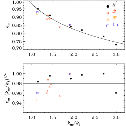
Figure 2: (Color online) Dependence of $\epsilon_{\rm m}{}$ on $k_{\rm m}$ for different sets of runs where either ${\cal Q}$ is varied (filled symbols), ${\cal B}$ is varied while keeping ${\cal R}=100$ (red diamonds), ${\cal B}$ is varied while keeping ${\cal L}=100$ (orange triangles), or ${\cal L}$ is varied (blue squares).

We note in passing that $k_{\rm m}$ enters neither in Eq. (22) nor in Eq. (23). However, $k_{\rm m}$ does enter if there is a magnetic helicity flux and it affects the time-dependent case, as is also clear from Eq. (10). Both cases will be considered below.

III.2 Effect of magnetic helicity flux

Next, we study cases where a diffusive magnetic helicity flux is included. In our model with perfectly conducting boundaries, the magnetic helicity flux vanishes on the boundaries, so no magnetic helicity is exported from the domain, but the divergence of the flux is finite and can thus modify the magnetic $\alpha$ effect. The same is true of periodic boundaries, where no magnetic helicity is exported, but the flux divergence is finite and can alleviate catastrophic quenching in dynamos driven by the kinetic $\alpha$ effect HB11 .

In Fig. 3 we compare profiles of $\overline{B}_{z}$ with and without magnetic helicity flux. It turns out that the $\kappa_{\alpha}$ term has the effect of smoothing out the resulting profile of $\overline{B}_{z}$. More interestingly, it can lead to a reversal of $\overline{B}_{z}$ at intermediate radii. For our reference run with ${\cal Q}=0.1$ (upper panel), the reversal is virtually absent at the rim of the cylinder. This is mainly because the pinch is so narrow; see Table LABEL:TF. However, when decreasing ${\cal Q}$ to 0.03, there is a clear reversal also at the outer rim (lower panel). However, decreasing ${\cal Q}$ to 0.01 does not increase the extent of the reversal. In none of these cases the field reversal is connected with a change of sign of $\alpha_{\rm red}$. Instead, $\alpha_{\rm red}$ is always found to be negative, even in the presence of a magnetic helicity flux. Thus, the sign reversal of $\overline{B}_{z}$ is therefore associated with a sign reversal of $\overline{J}_{z}$ at the same radius. Nevertheless, the reversal is still not very strong with $\min(\overline{B}_{z})/\max(\overline{B}_{z})\approx-0.07$, while in laboratory RFPs this ratio is typically $-0.2$ HPS89 .

Figure 3: Effect of magnetic helicity flux on equilibrium profiles of $\overline{B}_{z}$ for ${\cal Q}=0.1$ (upper panel) and ${\cal Q}=0.03$ (lower panel). Note the field reversal at the outer rim in the latter case.

Table 3: Values of $k_{\rm m}$ and $\epsilon_{\rm m}{}$ with and without magnetic helicity flux.

${\cal Q}\;$ 0.03 0.1 $\kappa_{\alpha}/\eta_{\rm t}$ 0 1 0 1 $k_{\rm m}R\;$ 4.63 4.50 3.51 3.32 $\epsilon_{\rm m}{}\;$ 0.84 0.83 0.91 0.92

III.3 Decay calculations

Next, we consider the case of a decaying magnetic field in the absence of an external electric field. In that case all components of $\overline{\bm{B}}$ must eventually decay to zero. The evolution of the magnetic energy of the resulting mean and fluctuating fields is shown in Fig. 4, together with the evolution of $k_{\rm m}$ and $\epsilon_{\rm m}{}$. At early times, when $\langle\overline{\bm{B}}^{2}\rangle\gg B_{\rm eq}^{2}$, the energy of the large-scale magnetic field decays at the resistive rate $\lambda=-2\eta k_{\rm m}^{2}$. During that time, the energy of the small-scale field stays approximately constant: the magnetically generated $\alpha$ effect almost exactly balances turbulent diffusion and the magnetic field can only decay at the resistive rate. However, at later times, when $\langle\overline{\bm{B}}^{2}\rangle\ll B_{\rm eq}^{2}$, the energy of the small-scale field decays with a negative growth rate $\lambda=-2\eta k_{\rm f}^{2}$, which then speeds up the decay of the energy of the large-scale magnetic field to a rate that is about $1.3\times\eta_{\rm t}k_{\rm m}^{2}$, where we have used the value $k_{\rm m}R=3.1$ that is relevant for the late-time decay. This value is also that obeying Taylor’s Tay74 postulated minimum energy state. Again, no reversal of the magnetic field is found, except in cases where there is an internal magnetic helicity flux in the system.

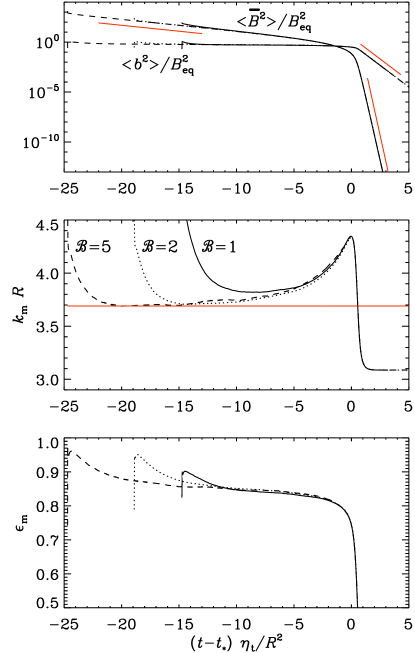
Figure 4: (Color online) Evolution of $\langle\overline{\bm{B}}^{2}\rangle/B_{\rm eq}^{2}$, $k_{\rm m}/k_{1}$, and $\epsilon_{\rm m}{}$ for different values of ${\cal B}$. Note that time is shifted by $t_{*}$, which is the time when $k_{\rm m}$ attains its second maximum. In the top panel, the red lines indicate resistive decay rate of the large-scale field at early times, resistive decay rate of the small-scale field at late times, and the turbulent decay rate of the large-scale field at late times.

IV Conclusions

The present work is an application of the dynamical quenching model of modern mean-field dynamo theory to magnetically driven and decaying turbulence in cylindrical geometry. In the driven case, an external electric field is applied, which leads to magnetic helicity injection at large scales. Such a situation has not yet been considered in the framework of mean-field theory. It turns out that in such a case there is a weak anti-correlation between the actual value of magnetic helicity of the mean field, $\epsilon_{\rm m}{}k_{\rm m}$, and the relative magnetic helicity $\epsilon_{\rm m}{}$ with $\epsilon_{\rm m}{}\sim k_{\rm m}^{-1/4}$. This weak anti-correlation is found to be independent of whether ${\cal Q}$, ${\cal B}$, or ${\cal L}$ are varied. No theoretical interpretation of this behavior has yet been offered. In the decaying case, we find that the decay rate is close to the resistive value when the field is strong, i.e., $\overline{B}>B_{\rm eq}$, and drops to the turbulent resistive value when the mean field becomes weaker. This behavior has also been found in earlier calculation of the decay of helical magnetic fields in Cartesian geometry YBR03 .

The original anticipation was that our model reproduces some features of the RFP that is studied in connection with fusion plasma confinement. It turns out that the expected field reversal that gives the RFP its name is found to require the presence of magnetic helicity fluxes. Without such fluxes, there is no reversal; see Fig. 3. Nevertheless, the reversal is rather weak compared with laboratory RFPs. This discrepancy can have several reasons. On the one hand, we have been working here with a model that has previously only been tested under simplifying circumstances in which there is turbulent dynamo action driven by kinetic helicity supply. It is therefore possible that the model has shortcomings that have not yet been fully understood. A related possibility is that the model is still basically valid, but our application to the RFP has been too crude. For example, the assumption of fixed values of $\eta_{\rm t}$ and $B_{\rm eq}$ is certainly quite simplistic. On the other hand, it is not clear that this simplification would really affect the outcome of the model in any decisive way. A different possibility is that the application of an external electric field is not representative of the RFP. However, an important basic idea behind the present setup has been to establish a model as simple as possible, that could be tested by performing corresponding three-dimensional simulations of a similar setup. This has not yet been attempted, but this would clearly constitute a natural next step to take.

- (1) H. K. Moffatt, Magnetic field generation in electrically conducting fluids. Cambridge University Press, Cambridge (1978).
- (2) F. Krause and K.-H. Rädler, Mean-field magnetohydrodynamics and dynamo theory. Pergamon Press, Oxford (1980).
- (3) T. Ogino, J. Geophys. Res. 91, 6791 (1986).
- (4) H. Ji, S. C. Prager, A. F. Almagri, J. S. Sarff, and H. Toyama, Phys. Plasmas 3, 1935 (1996).
- (5) R. Monchaux, M. Berhanu, M. Bourgoin, et al., Phys. Rev. Lett. 98, 044502 (2007).
- (6) H. A. B. Bodin and A. A. Newton, Nuclear Fusion 20, 1255 (1980).
- (7) J. B. Taylor, Phys. Rev. Lett. 58, 741 (1986).
- (8) E. G. Blackman and H. Ji, Mon. Not. R. Astron. Soc. 369, 1837 (2006).
- (9) A. Pouquet, U. Frisch, and J. Léorat, J. Fluid Mech. 77, 321 (1976).
- (10) G. B. Field and E. G. Blackman, Astrophys. J. 572, 685 (2002).
- (11) E. G. Blackman and A. Brandenburg, Astrophys. J. 579, 359 (2002).
- (12) K. Subramanian, Bull. Astr. Soc. India 30, 715 (2002).
- (13) N. I. Kleeorin and A. A. Ruzmaikin, Magnetohydrodynamics 18, 116 (1982).
- (14) A. Brandenburg and K. Subramanian, Astron. Nachr. 326, 400 (2005).
- (15) A. Brandenburg and C. Sandin, Astron. Astrophys. 427, 13 (2004).
- (16) A. Brandenburg, Astrophys. J. 625, 539 (2005).
- (17) H. Ji and S. C. Prager, Magnetohydrodynamics 38, 191 (2002). astro-ph/0110352
- (18) J. B. Taylor, Phys. Rev. Lett. 33, 1139 (1974).
- (19) A. Y. Aydemir and D. C. Barnes, Phys. Rev. Lett. 52, 930 (1984).
- (20) T. A. Yousef, A. Brandenburg, and G. Rüdiger, Astron. Astrophys. 411, 321 (2003).
- (21) D. D. Schnack, E. J. Caramana, and R. A. Nebel, Phys. Fluids 28, 321 (1985).
- (22) H.-E. Sätherblom, S. Mazur, and P. Nordlund, Plasmas Phys. Contr. Fusion 38, 2205 (1996).
- (23) S. Cappello, D. Bonfiglio, and D. F. Escande, Phys. Plasmas 13, 056102 (2006).
- (24) H. R. Strauss, Phys. Fluids 28, 2786 (1985).
- (25) A. Bhattacharjee and E. Hameiri, Phys. Rev. Lett. 57, 206 (1986).
- (26) H. Ji, Phys. Rev. Lett. 83, 3198 (1999).
- (27) N. Kleeorin, I. Rogachevskii, and A. Ruzmaikin, Astron. Astrophys. 297, 159 (1995).
- (28) K. Subramanian and A. Brandenburg, Astrophys. J. 648, L71 (2006).
- (29) A. Hubbard and A. Brandenburg, Geophys. Astrophys. Fluid Dynam. 104, 577 (2010).
- (30) D. Mitra, S. Candelaresi, P. Chatterjee, R. Tavakol, and A. Brandenburg, Astron. Nachr. 331, 130 (2010).
- (31) A. Brandenburg, W. Dobler, and K. Subramanian, Astron. Nachr. 323, 99 (2002).
- (32) Y. L. Ho, S. C. Prager, D. D.Schnack, Phys. Rev. Lett. 62, 1504 (1989).
- (33) A. Brandenburg, K.-H. Rädler, M. Rheinhardt, and K. Subramanian, Astrophys. J. 676, 740 (2008).
- (34) A. Hubbard and A. Brandenburg, Astrophys. J. 727, 11 (2011).