Random stable laminations of the disk

Abstract

We study large random dissections of polygons. We consider random dissections of a regular polygon with $n$ sides, which are chosen according to Boltzmann weights in the domain of attraction of a stable law of index $\theta\in(1,2]$. As $n$ goes to infinity, we prove that these random dissections converge in distribution toward a random compact set, called the random stable lamination. If $\theta=2$, we recover Aldous’ Brownian triangulation. However, if $\theta\in(1,2)$, large faces remain in the limit and a different random compact set appears. We show that the random stable lamination can be coded by the continuous-time height function associated to the normalized excursion of a strictly stable spectrally positive Lévy process of index $\theta$. Using this coding, we establish that the Hausdorff dimension of the stable random lamination is almost surely $2-1/\theta$.

Introduction

In this article we study large random dissections of polygons. A dissection of a polygon is the union of the sides of the polygon and of a collection of diagonals that may intersect only at their endpoints. The faces are the connected components of the complement of the dissection in the polygon. The particular case of triangulations (when all faces are triangles) has been extensively studied in the literature. For every integer $n\geq 3$, let $P_{n}$ be the regular polygon with $n$ sides whose vertices are the $n$th roots of unity. It is well known that the number of triangulations of $P_{n}$ is the Catalan number of order $n-2$. In the general case, where faces of degree greater than three are allowed, there is no known explicit formula for the number of dissections of $P_{n}$, although an asymptotic estimate is known (see FlajoletNoy , CK ). Probabilistic aspects of uniformly distributed random triangulations have been investigated; see, for example, the articles GaoWormald1 , GaoWormald2 which study graph-theoretical properties of uniform triangulations (such as the maximal vertex degree or the number of vertices of degree $k$). Graph-theoretical properties of uniform dissections of $P_{n}$ have also been studied, extending the previously mentioned results for triangulations (see Berna , CK ).

From a more geometrical point of view, Aldous Aldous , Aldous2 studied the shape of a large uniform triangulation viewed as a random compact subset of the closed unit disk. See also the work of Curien and Le Gall CLG , who discuss a random continuous triangulation (different from Aldous’ one) obtained as a limit of random dissections constructed recursively. Our goal is to generalize Aldous’ result by studying the shape of large random dissections of $P_{n}$, viewed as random variables with values in the space of all compact subsets of the disk, which is equipped with the usual Hausdorff metric.

Let us state more precisely Aldous’ results. Denote by $\mathfrak{t}_{n}$ a uniformly distributed random triangulation of $P_{n}$. There exists a random compact subset $\mathfrak{t}$ of the closed unit disk $\overline{\mathbb{D}}$ such that the sequence $(\mathfrak{t}_{n})$ converges in distribution toward $\mathfrak{t}$. The random compact set $\mathfrak{t}$ is a continuous triangulation, in the sense that $\overline{\mathbb{D}}\setminus\mathfrak{t}$ is a disjoint union of open triangles whose vertices belong to the unit circle. Aldous also explains how $\mathfrak{t}$ can be explicitly constructed using the Brownian excursion and computes the Hausdorff dimension of $\mathfrak{t}$, which is equal almost surely to $3/2$ (see also LGP ).

In this work, we propose to study the following generalization of this model. Consider a probability distribution $(\mu_{j})_{j\geq 0}$ on the nonnegative integers such that $\mu_{1}=0$ and the mean of $\mu$ is equal to $1$. We suppose that $\mu$ is in the domain of attraction of a stable law of index $\theta\in(1,2]$. For every integer $n\geq 2$, let $\mathbb{L}_{n}$ be the set of all dissections of $P_{n+1}$, and consider the following Boltzmann probability measure on $\mathbb{L}_{n}$ associated to the weights $(\mu_{j})$:

$$\mathbb{P}^{\mu}_{n}(\omega)=\frac{1}{Z_{n}}\prod_{f\ \mathrm{face\ of}\ \omega}\mu_{\deg(f)-1},\qquad\omega\in\mathbb{L}_{n},$$

where $\deg(f)$ is the degree of the face $f$, that is, the number of edges in the boundary of $f$, and $Z_{n}$ is a normalizing constant. Note that the definition of $\mathbb{P}^{\mu}_{n}$ involves only $\mu_{2},\mu_{3},\ldots,$ and $\mu_{0}$ is the missing constant to obtain a probability measure. Under appropriate conditions on $\mu$, this definition makes sense for all sufficiently large integers $n$. Let us mention two important special cases. If $\mu_{0}=2-\sqrt{2}$ and $\mu_{i}=((2-\sqrt{2})/2)^{i-1}$ for every $i\geq 2$, one easily checks that $\mathbb{P}^{\mu}_{n}$ is uniform over $\mathbb{L}_{n}$. If $p\geq 3$ is an integer and if $\mu_{0}=1-1/(p-1)$, $\mu_{p-1}=1/(p-1)$ and $\mu_{i}=0$ otherwise, $\mathbb{P}^{\mu}_{n}$ is uniform over dissections of $\mathbb{L}_{n}$ with all faces of degree $p$ (in that case, we must restrict our attention to values of $n$ such that $n-1$ is a multiple of $p-2$, but our results carry over to this setting).

We are interested in the following problem. Let $\mathfrak{l}_{n}$ be a random dissection distributed according to $\mathbb{P}_{n}$. Does the sequence $(\mathfrak{l}_{n})$ converge in distribution to a random compact subset of $\overline{\mathbb{D}}$? Let us mention that this setting is inspired by LGM , where Le Gall and Miermont consider random planar maps chosen according to a Boltzmann probability measure, and show that if the Boltzmann weights do not decrease sufficiently fast, large faces remain in the scaling limit. We will see that this phenomenon occurs in our case as well.

In our main result Theorem 3.1, we first consider the case where the variance of $\mu$ is finite and then show that $\mathfrak{l}_{n}$ converges in distribution to Aldous’ Brownian triangulation as $n\rightarrow\infty$. This extends Aldous’ theorem to random dissections which are not necessarily triangulations. For instance, we may let $\mathfrak{l}_{n}$ be uniformly distributed over the set of all dissections whose faces are all quadrangles (or pentagons, or hexagons, etc.). As noted above, this requires that we restrict our attention to a subset of values of $n$, but the convergence of $\mathfrak{l}_{n}$ toward the Brownian triangulation still holds. This maybe surprising result comes from the fact that certain sides of the squares (or of the pentagons, or of the hexagons, etc.) degenerate in the limit. See also the recent paper CK for other classes of noncrossing configurations of the polygon that converge to the Brownian triangulation.

On the other hand, if $\mu$ is in the domain of attraction of a stable law of index $\theta\in(1,2)$, Theorem 3.1 shows that $(\mathfrak{l}_{n})$ converges in distribution to another random compact subset $\mathfrak{l}$ of $\overline{\mathbb{D}}$, which we call the $\theta$-stable random lamination of the disk. The random compact subset $\mathfrak{l}$ is the union of the unit circle and of infinitely many noncrossing chords, which can be constructed as follows. Let $X^{\mathrm{exc}}=(X^{\mathrm{exc}}_{t})_{0\leq t\leq 1}$ be the normalized excursion of the strictly stable spectrally positive Lévy process of index $\theta$ (see Section 2.1 for a precise definition). For $0\leq s<t\leq 1$, we set $s\mathop{\simeq}^{X^{\mathrm{exc}}}t$ if $t=\inf\{u>s;X^{\mathrm{exc}}_{u}\leq X^{\mathrm{exc}}_{s-}\}$, and $s\mathop{\simeq}^{X^{\mathrm{exc}}}s$ by convention. Then

$$\mathfrak{l}=\bigcup_{s\mathop{\simeq}^{X^{\mathrm{exc}}}t}\bigl{[}e^{-2\mathrm{i}\pi s},e^{-2\mathrm{i}\pi t}\bigr{]},$$ (1)

where $[u,v]$ stands for the line segment between the two complex numbers $u$ and $v$. In particular, the latter set is compact, which is not obvious a priori.

In order to study fine properties of the set $\mathfrak{l}$, we derive an alternative representation in terms of the so-called height process $H^{\mathrm{exc}}=(H^{\mathrm{exc}}_{t})_{0\leq t\leq 1}$ associated with $X^{\mathrm{exc}}$ (see Duquesne , DuquesneLG for the definition and properties of $H^{\mathrm{exc}}$). Note that $H^{\mathrm{exc}}$ is a random continuous function on $[0,1]$ that vanishes at $0$ and at $1$ and takes positive values on $(0,1)$. Then Theorem 4.5 states that

$$\mathfrak{l}=\bigcup_{s\mathop{\thickapprox}^{H^{\mathrm{exc}}}t}\bigl{[}e^{-2\mathrm{i}\pi s},e^{-2\mathrm{i}\pi t}\bigr{]},$$ (2)

where, for $s,t\in[0,1]$, $s\mathop{\thickapprox}^{H^{\mathrm{exc}}}t$ if $H^{\mathrm{exc}}_{s}=H^{\mathrm{exc}}_{t}$ and $H^{\mathrm{exc}}_{r}>H^{\mathrm{exc}}_{s}$ for every $r\in(s\wedge t,s\vee t)$, or if $(s,t)$ is a limit of pairs satisfying these properties. This is very closely related to the equivalence relation used to define the so-called stable tree, which is coded by $H^{\mathrm{exc}}$ (see Duquesne ). The representation (2) thus shows that the $\theta$-stable random lamination is connected to the $\theta$-stable tree in the same way as the Brownian triangulation is connected to the Brownian CRT (see Aldous2 for applications of the latter connection). The representation (2) also allows us to establish that the Hausdorff dimension of $\mathfrak{l}$ is almost surely equal to $2-1/\theta$. Note that for $\theta=2$, we obtain a Hausdorff dimension equal to $3/2$, which is consistent with Aldous’ result. Additionally, we verify that the Hausdorff dimension of the set of endpoints of all chords in $\mathfrak{l}$ is equal to $1-1/\theta$.

Finally, we derive precise information about the faces of $\mathfrak{l}$, which are the connected components of the complement of $\mathfrak{l}$ in the closed unit disk. When $\theta=2$, we already noted that all faces are triangles. On the other hand, when $\theta\in(1,2)$, each face is bounded by infinitely many chords. We prove more precisely that the set of extreme points of the closure of a face (or, equivalently, the set of points of the closure that lie on the circle) has Hausdorff dimension $1/\theta$.

Let us now sketch the main techniques and arguments used to establish the previous assertions. A key ingredient is the fact that the dual graph of $\mathfrak{l}_{n}$ is a Galton–Watson tree conditioned on having $n$ leaves. In our previous work K , we establish limit theorems for Galton–Watson trees conditioned on their number of leaves and, in particular, we prove an invariance principle stating that the rescaled Lukasiewicz path of a Galton–Watson tree conditioned on having $n$ leaves converges in distribution to $X^{\mathrm{exc}}$ (see Theorem 3.3 below). Using this result, we are able to show that $\mathfrak{l}_{n}$ converges toward the random compact set $\mathfrak{l}$ described by (1). The representation (2) then follows from relations between $X^{\mathrm{exc}}$ and $H^{\mathrm{exc}}$. Finally, we use (2) to verify that the Hausdorff dimension of $\mathfrak{l}$ is almost surely equal to $2-1/\theta$. This calculation relies in part on the time-reversibility of the process $H^{\mathrm{exc}}$. It seems more difficult to derive the Hausdorff dimension of $\mathfrak{l}$ from the representation (1).

The paper CK develops a number of applications of the present work to enumeration problems and asymptotic properties of uniformly distributed random dissections.

The paper is organized as follows. In Section 1 we present the discrete framework. In particular, we introduce Galton–Watson trees and their coding functions. In Section 2 we discuss the normalized excursion of the strictly stable spectrally positive Lévy process of index $\theta$ and its associated lamination $L(X^{\mathrm{exc}})$. In Section 3 we prove that $(\mathfrak{l}_{n})$ converges in distribution toward $L(X^{\mathrm{exc}})$. In Section 4 we start by introducing the continuous-time height process $H^{\mathrm{exc}}$ associated to $X^{\mathrm{exc}}$ and we then show that $L(X^{\mathrm{exc}})$ can be coded by $H^{\mathrm{exc}}$. In Section 5 we use the time-reversibility of $H^{\mathrm{exc}}$ to calculate the Hausdorff dimension of the stable lamination.

Throughout this work, the notation $\overline{A}$ stands for the closure of a subset $A$ of the plane.

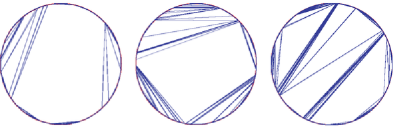
Figure 1: Random dissections of $P_{27183}$ for $\theta=1.1$, of $P_{11655}$ for $\theta=1.5$ and of $P_{20999}$ for $\theta=1.9$.

1 The discrete setting: Dissections and trees

1.1 Boltzmann dissections

Definition 1.1.

A dissection of a polygon is the union of the sides of the polygon and of a collection of diagonals that may intersect only at their endpoints. A face $f$ of a dissection $\omega$ of a polygon $P$ is a connected component of the complement of $\omega$ inside $P$; its degree, denoted by $\deg(f)$, is the number of sides surrounding $f$. See Figure 1 for an example.

Let $(\mu_{i})_{i\geq 2}$ be a sequence of nonnegative real numbers. For every integer $n\geq 3$, let $P_{n}$ be the regular polygon of the plane whose vertices are the $n$th roots of unity. For every $n\geq 2$, let $\mathbb{L}_{n}$ be the set of all dissections of $P_{n+1}$. Note that $\mathbb{L}_{n}$ is a finite set. Let $\mathbb{L}=\bigcup_{n\geq 2}\mathbb{L}_{n}$ be the set of all dissections. A weight $\pi(\omega)$ is associated to each dissection $\omega\in\mathbb{L}_{n}$ by setting

$$\pi(\omega)=\prod_{f\ \mathrm{face\ of}\ \omega}\mu_{\deg(f)-1}.$$

We define a probability measure on $\mathbb{L}_{n}$ by normalizing these weights. More precisely, we set

$$Z_{n}=\sum_{w\in\mathbb{L}_{n}}\pi(w),$$ (3)

and for every $n\geq 2$ such that $Z_{n}>0$,

$$\mathbb{P}^{\mu}_{n}(\omega)=\frac{1}{Z_{n}}\pi(\omega)$$

for $\omega\in\mathbb{L}_{n}$.

We are interested in the asymptotic behavior of random dissections sampled according to $\mathbb{P}^{\mu}_{n}$. Let $\overline{\mathbb{D}}$ be the closed unit disk of the complex plane and let $\mathcal{C}$ be the set of all compact subsets of $\overline{\mathbb{D}}$. We equip $\mathcal{C}$ with the Hausdorff distance $d_{H}$, so that $(\mathcal{C},d_{H})$ is a compact metric space. In the following, we will always view a dissection as an element of this metric space.

We are interested in the following question. For every $n\geq 2$ such that $Z_{n}>0$, let $\mathfrak{l}_{n}$ be a random dissection distributing according to $\mathbb{P}^{\mu}_{n}$. Does there exist a limiting random compact set $\mathfrak{l}$ such that $\mathfrak{l}_{n}$ converges in distribution toward $\mathfrak{l}$?

We shall answer this question for some specific families of sequences $(\mu_{i})_{i\geq 2}$ defined as follows. Let $\theta\in(1,2]$. We say that a sequence of nonnegative real numbers $(\mu_{j})_{j\geq 2}$ satisfies the condition $(H_{\theta})$ if: [$-$]

$\mu$ is critical, meaning that $\sum_{i=2}^{\infty}i\mu_{i}=1$. Note that this condition implies $\sum_{i=2}^{\infty}\mu_{i}<1$.

Set $\mu_{1}=0$ and $\mu_{0}=1-\sum_{i=2}^{\infty}\mu_{i}$. Then $(\mu_{j})_{j\geq 0}$ is a probability measure in the domain of attraction of a stable law of index $\theta$.

Recall that the second condition is equivalent to saying that if $X$ is a random variable such that $\mathbb{P}[X=j]=\mu_{j}$ for $j\geq 0$, then either $X$ has finite variance or $\mathbb{P}[X\geq j]=j^{-\theta}L(j)$, where $L$ is a function such that $\lim_{x\rightarrow\infty}L(tx)/L(x)=1$ for all $t>0$ (such a function is called slowly varying at infinity). We refer to Bingham or Durrett , Chapter 3.7, for details.

1.2 Random dissections and Galton–Watson trees

In this subsection we explain how to associate a dual object to a dissection. This dual object is a finite rooted ordered tree. The study of large random dissections will then boil down to the study of large Galton–Watson trees, which is a more familiar realm.

Definition 1.2.

Let $\mathbb{N}=\{0,1,\ldots\}$ be the set of all nonnegative integers, $\mathbb{N}^{*}=\{1,2,\ldots\}$, and let $U$ be the set of labels

$$U=\bigcup_{n=0}^{\infty}\bigl{(}\mathbb{N}^{*}\bigr{)}^{n},$$

where by convention $(\mathbb{N}^{*})^{0}=\{\varnothing\}$. An element of $U$ is a sequence $u=u_{1}\cdots u_{m}$ of positive integers, and we set $|u|=m$, which represents the “generation” of $u$. If $u=u_{1}\cdots u_{m}$ and $v=v_{1}\cdots v_{n}$ belong to $U$, we write $uv=u_{1}\cdots u_{m}v_{1}\cdots v_{n}$ for the concatenation of $u$ and $v$. In particular, note that $u\varnothing=\varnothing u=u$. Finally, a rooted ordered tree $\tau$ is a finite subset of $U$ such that: [(3)]

$\varnothing\in\tau$;

if $v\in\tau$ and $v=uj$ for some $j\in\mathbb{N}^{*}$, then $u\in\tau$;

for every $u\in\tau$, there exists an integer $k_{u}(\tau)\geq 0$ such that, for every $j\in\mathbb{N}^{*}$, $uj\in\tau$ if and only if $1\leq j\leq k_{u}(\tau)$. In the following, by tree we will always mean rooted ordered tree. We denote the set of all trees by $\mathbb{T}$. We will often view each vertex of a tree $\tau$ as an individual of a population whose $\tau$ is the genealogical tree. The total progeny of $\tau$, Card$(\tau)$, will be denoted by $\zeta(\tau)$. A leaf of a tree $\tau$ is a vertex $u\in\tau$ such that $k_{u}(\tau)=0$. The total number of leaves of $\tau$ will be denoted by $\lambda(\tau)$. If $\tau$ is a tree and $u\in\tau$, we define the shift of $\tau$ at $u$ by $T_{u}\tau=\{v\in U;uv\in\tau\}$, which is itself a tree.

Given a dissection $\omega\in\mathbb{L}_{n}$, we construct a (rooted ordered) tree $\phi(\omega)$ as follows: consider the dual graph of $\omega$, obtained by placing a vertex inside each face of $\omega$ and outside each side of the polygon $P_{n+1}$ and by joining two vertices if the corresponding faces share a common edge, thus giving a connected graph without cycles. Then remove the dual edge intersecting the side $[1,e^{{2\mathrm{i}\pi}/{(n+1)}}]$ of $P_{n}$. Finally, root the graph at the dual vertex corresponding to the face adjacent to the side $[1,e^{{2i\pi}/{(n+1)}}]$ (see Figure 2). The planar structure now allows us to associate a tree $\phi(\omega)$ to this graph, in a way that should be obvious from Figure 2. Note that $k_{u}(\phi(\omega))\neq 1$ for every $u\in\phi(\omega)$.

For every integer $n\geq 2$, let $\mathbb{T}_{(n)}$ stand for the set of all trees $\tau\in\mathbb{T}$ with exactly $n$ leaves and such that $k_{u}(\tau)\neq 1$ for every $u\in\tau$. The preceding construction provides a bijection $\phi$ from $\mathbb{L}_{n}$ onto $\mathbb{T}_{(n)}$. Furthermore, if $\tau=\phi(\omega)$ for $\omega\in\mathbb{L}_{n}$, there is a one-to-one correspondence between internal vertices of $\tau$ and faces of $\omega$, such that if $u$ is an internal vertex of $\tau$ and $f$ is the associated face of $\omega$, we have $\deg f=k_{u}(\tau)+1$. The latter property should be clear from our construction.

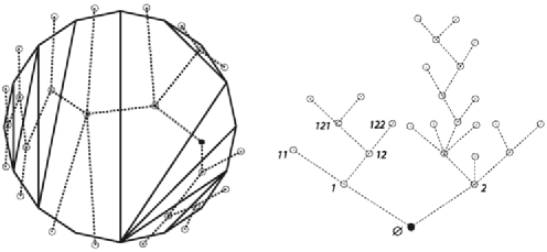
Figure 2: The dual tree of a dissection, rooted at the bold vertex.

Definition 1.3.

Let $\rho$ be a probability measure on $\mathbb{N}$ with mean less than or equal to $1$ and such that $\rho(1)<1$. The law of the Galton–Watson tree with offspring distribution $\rho$ is the unique probability measure $\mathbb{P}_{\rho}$ on $\mathbb{T}$ such that: [(1)]

$\mathbb{P}_{\rho}[k_{\varnothing}=j]=\rho(j)$ for $j\geq 0$;

for every $j\geq 1$ with $\rho(j)>0$, the shifted trees $T_{1}\tau,\ldots,T_{j}\tau$ are independent under the conditional probability $\mathbb{P}_{\rho}[\cdot|k_{\varnothing}=j]$ and their conditional distribution is $\mathbb{P}_{\rho}$.

A random tree with distribution $\mathbb{P}_{\rho}$ will sometimes be called a $GW_{\rho}$ tree.

Proposition 1.4

Let $(\mu_{j})_{j\geq 2}$ be a sequence of nonnegative real numbers such that $\sum_{j=2}^{\infty}j\mu_{j}=1$. Put $\mu_{1}=0$ and $\mu_{0}=1-\sum_{j=2}^{\infty}\mu_{j}$ so that $\mu=(\mu_{j})_{j\geq 0}$ defines a probability measure on $\mathbb{N}$, which satisfies the assumptions of Definition 1.3. Let $n\geq 2$ and let $Z_{n}$ be defined as in (3). Then $Z_{n}>0$ if, and only if, $\mathbb{P}_{\mu}[\lambda(\tau)=n]>0$. Assume that this condition holds. Then if $\mathfrak{l}_{n}$ is a random dissection distributed according to $\mathbb{P}^{\mu}_{n}$, the tree $\phi(\mathfrak{l}_{n})$ is distributed according to $\mathbb{P}_{\mu}[\cdot|\lambda(\tau)=n]$.

Let $\tau\in\mathbb{T}_{(n)}$ and $\omega=\phi^{-1}(\tau)$. Then

$$\mathbb{P}_{\mu}(\tau)=\prod_{u\in\tau}\mu_{k_{u}(\tau)}=\mu_{0}^{n}\prod_{f\ \mathrm{face\ of}\ \omega}\mu_{\deg(f)-1}=\mu_{0}^{n}\pi(\omega).$$ (4)

The first equality is a well-known property of Galton–Watson trees (see, e.g., Proposition 1.4 in RandomTrees ). The second one follows from the observations preceding Definition 1.3, and the last one is the definition of $\pi(\omega)$. From (4), we now get that $\mathbb{P}_{\mu}(\mathbb{T}_{(n)})=\mu_{0}^{n}Z_{n}$, and then (if these quantities are positive) that $\mathbb{P}_{\mu}(\tau\mid\mathbb{T}_{(n)})=\mathbb{P}^{\mu}_{n}(\omega)$, giving the last assertion of the proposition.

Remark 1.5.

The preceding proposition will be a major ingredient of our study. We will derive information about the random dissection $\mathfrak{l}_{n}$ (when $n\rightarrow\infty$) from asymptotic results for the random trees $\phi(\mathfrak{l}_{n})$. To this end, we will assume that $(\mu_{j})_{j\geq 2}$ satisfies condition $(H_{\theta})$ for some $\theta\in(1,2]$, which will allow us to use the limit theorems of K for Galton–Watson trees conditioned to have a (fixed) large number of leaves.

1.3 Coding trees and dissections

In the previous subsection we have seen that certain random dissections are coded by conditioned Galton–Watson trees. We now explain how trees themselves can be coded by two functions, called, respectively, the Lukasiewicz path and the height function (see Figures 3 and 4 for an example). These codings are crucial in the understanding of large Galton–Watson trees and thus of large random dissections.

We write $u<v$ for the lexicographical order on the set $U$ (e.g., $\varnothing<1<21<22$). In the following, we will denote the children of a tree $\tau$ listed in lexicographical order by $\varnothing=u(0)<u(1)<\cdots<u(\zeta(\tau)-1)$.

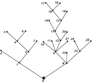
Figure 3: The dual tree $\tau$ associated to the dissection of Figure 2 with its vertices indexed in lexicographical order. Here, $\zeta(\tau)=26$.

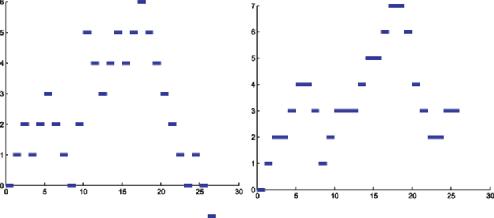
Figure 4: The Lukasiewicz path $(W_{u}(\tau),0\leq u\leq\zeta(\tau))$ and the height function $(H_{u}(\tau),0\leq u<\zeta(\tau)$ of $\tau$.

Definition 1.6.

Let $\tau\in\mathbb{T}$. The height process $H(\tau)=(H_{n}(\tau),0\leq n<\zeta(\tau))$ is defined, for $0\leq n<\zeta(\tau)$, by $H_{n}(\tau)=|u(n)|$. The Lukasiewicz path $W(\tau)=(W_{n}(\tau),0\leq n\leq\zeta(\tau))$ is defined by $W_{0}(\tau)=0$ and $W_{n+1}(\tau)=W_{n}(\tau)+k_{u(n)}(\tau)-1$ for $0\leq n\leq\zeta(\tau)-1$.

It is easy to see that $W_{n}(\tau)\geq 0$ for $0\leq n<\zeta(\tau)$ but $W_{\zeta}(\tau)=-1$ (see, e.g., RandomTrees ).

Consider a dissection $\omega$, its dual tree $\tau=\phi(\omega)$ and $W(\tau)$, the associated Lukasiewicz path. We now explain how to reconstruct $\omega$ from $W(\tau)$. As a first step, recall that an internal vertex $u$ of $\tau$ is associated to a face $f$ of $\omega$, and that the chords bounding $f$ are in bijection with the dual edges linking $u$ to its children and to its parent. The following proposition explains how to find all the children of a given vertex of $\tau$ using only $W$ or $H$, and will be useful to construct the edges linking the vertex $u\in\tau$ to its children.

Proposition 1.7

Let $\tau\in\mathbb{T},$ and let $u(0),\ldots,u(\zeta(\tau)-1)$ be as above the vertices of $\tau$ listed in lexicographical order. Fix $n\in\{0,1,\ldots,\zeta(\tau)-1\}$ such that $k_{u(n)}(\tau)>0$ and set $k=k_{u(n)}(\tau)$. [(ii)]

Let $s_{1},\ldots,s_{k}\in\{0,1,\ldots,\zeta(\tau)-1\}$ be defined by setting $s_{i}=\inf\{l\geq n+1;W_{l}(\tau)=W_{n+1}(\tau)-(i-1)\}$ for $1\leq i\leq k$ (in particular, $s_{1}=n+1$). Then $u(s_{1}),u(s_{2}),\ldots,u(s_{k})$ are the children of $u(n)$ listed in lexicographical order.

We have $H_{s_{1}}(\tau)=H_{s_{2}}(\tau)=\cdots=H_{s_{k}}(\tau)=H_{n}(\tau)+1$. Furthermore, for $1\leq i\leq k-1$,

$$H_{j}(\tau)>H_{s_{i}}(\tau)=H_{s_{i+1}}(\tau)\qquad\forall j\in(s_{r},s_{r+1})\cap\mathbb{N}.$$

We leave this as an exercise (or see the proof of Proposition 1.2 in RandomTrees ) and encourage the reader to visualize what this means on Figure 4.

In a second step, we explain how to reconstruct the dissection from the Lukasiewicz path of its dual tree.

Proposition 1.8

Let $\zeta\geq 2$ be an integer and let $Z=(Z_{n},0\leq n\leq\zeta)$ be a sequence of integers such that $Z_{0}=0$, $Z_{\zeta}=-1$, $Z_{k}\geq 0$ for $0\leq k<\zeta$ and $Z_{i+1}-Z_{i}\in\{-1,1,2,3,\ldots\}$ for $0\leq i<\zeta$. For $0\leq i<\zeta$, set $X_{i}=Z_{i+1}-Z_{i}$ and, for $1\leq i\leq\zeta$,

$$\Lambda(i)=\operatorname{Card}\{0\leq j<i;X_{j}=-1\}.$$

For every integer $i\in\{0,1,\ldots,\zeta(\tau)-1\}$ such that $X_{i}\geq 1$, set $k_{i}=X_{i}+1$ and let $s^{i}_{1},\ldots,s^{i}_{k_{i}+2}$ be defined by $s^{i}_{1}=s^{i}_{k_{i}+2}=i+1$ and $s^{i}_{m+1}=\inf\{l\geq i+1;Z_{l}=Z_{i+1}-m\}$ for $1\leq m\leq k_{i}$. Then the set $D(Z)$ defined by

$$D(Z)=\bigcup_{i;X_{i}\geq 1}\bigcup_{j=1}^{k_{i}+1}\biggl{[}\exp\biggl{(}-2\mathrm{i}\pi\frac{\Lambda(s_{j}^{i})}{\Lambda(\zeta)+1}\biggr{)},\exp\biggl{(}-2\mathrm{i}\pi\frac{\Lambda(s_{j+1}^{i})}{\Lambda(\zeta)+1}\biggr{)}\biggr{]}$$ (5)

is a dissection of the polygon $P_{\Lambda(\zeta)+1}$ called the dissection coded by $Z$.

Note that if $\tau$ is a tree (different from the trivial tree $\{\varnothing\}$), if $u(0),\ldots,$ $u(\zeta(\tau)-1)$ are its vertices listed in lexicographical order and $Z=W(\tau)$, then $\Lambda(i)$ is the number of leaves among $u(0),u(1),\ldots u(i-1)$ [in particular, $\Lambda(\zeta)$ is the number of leaves of $\tau$], $k_{i}$ is the number of children of $u(i)$, and $s^{i}_{m}$ is the index of the $m$th child of $u(i)$ for $1\leq m\leq k_{i}$.

First notice that, for all pairs $(i,j)$ occurring in the union of (5), we have $\Lambda(s^{i}_{j})\neq\Lambda(s^{i}_{j+1})$. We then check that all edges of the polygon $P_{\Lambda(\zeta)+1}$ appear in the right-hand side of (5). To this end, fix $\ell\in\{0,1,\ldots,\Lambda(\zeta)-1\}$. Then there is a unique integer $k\in\{1,2,\ldots,\zeta-1\}$ such that $X_{k}=-1$ and $\Lambda(k)=\ell$. Set

$$i=\sup\bigl{\{}j\in\{0,1,\ldots,k-1\}\dvtx Z_{j}\leq Z_{k}\bigr{\}}$$

and $m=Z_{i+1}-Z_{k}+1$. Notice that $1\leq m\leq k_{i}$ since $Z_{k}\geq Z_{i}$ by construction. It is now a simple matter to verify that $s^{i}_{m}=k$ and $s^{i}_{m+1}=k+1$. Recalling that $\Lambda(k)=\ell$ and $\Lambda(k+1)=\ell+1$, we get that the line segment

$$\biggl{[}\exp\biggl{(}-2\mathrm{i}\pi\frac{\ell}{\Lambda(\zeta)+1}\biggr{)},\exp\biggl{(}-2\mathrm{i}\pi\frac{\ell+1}{\Lambda(\zeta)+1}\biggr{)}\biggr{]}$$

appears in the right-hand side of (5). We therefore get that $D(Z)$ contains all edges of $P_{\Lambda(\zeta)+1}$ with the possible exception of the edge $[1,\exp(-2\mathrm{i}\pi\frac{\Lambda(\zeta)}{\Lambda(\zeta)+1})]$. However, the latter edge also appears in the union of (5), taking $i=0$ and $j=k_{0}+1$ and noting that $s^{0}_{k_{0}+1}=\zeta$ and $s^{0}_{k_{0}+2}=1$.

Next suppose that $0\leq i<\zeta,0\leq i^{\prime}<\zeta$ are such that $k_{i}\geq 1,k_{i^{\prime}}\geq 1$. Let $j\in\{1,\ldots,k_{i}+1\}$, $j^{\prime}\in\{1,\ldots,k_{i^{\prime}}+1\}$. If $(i,j)\neq(i^{\prime},j^{\prime})$, one easily checks that either the intervals $(s^{i}_{j},s^{i}_{j+1})$ are disjoint or one of them is contained in either one. It follows that the chords corresponding, respectively, to $(i,j)$ and to $(i^{\prime},j^{\prime})$ in the union of (5) are noncrossing. Hence, $D(Z)$ is a dissection.

Lemma 1.9

For every dissection $\omega\in\mathbb{L}$, we have $D(W(\phi(\omega)))=\omega$. In other words, a dissection is equal to the dissection coded by the Lukasiewicz path of its dual tree.

This is a consequence of our construction. Suppose that $\omega\in\mathbb{L}_{n}$, for some $n\geq 2$, and set $\tau=\phi(\omega)$. Fix a face $f$ of $\omega$ and the corresponding dual vertex $u(i)\in\phi(\omega)$ (recall that the faces of $f$ are in one-to-one correspondence with the internal vertices of $\tau$). Denote the Lukasiewicz path of $\tau$ by $Z=W(\tau)$. First notice that the degree of $f$ is equal to $1+k_{u(i)}=Z_{i+1}-Z_{i}+2$, where $k_{u(i)}$ is the number of children of $u(i)$. To simplify notation, set $k_{i}=k_{u(i)}$. Let $s^{i}_{1},\ldots,s^{i}_{k_{i}+2}$ be defined as in Proposition 1.8. By Proposition 1.7, $u(s^{i}_{1}),u(s^{i}_{2}),\ldots,u(s^{i}_{k_{i}})$ are the children of $u(i)$.

As in Proposition 1.8, we set, for every $1\leq i\leq\zeta$, $\Lambda(i)=\operatorname{Card}\{0\leq j<i;Z_{j+1}-Z_{j}=-1\}$, which represents the number of leaves among the first $i$ vertices of $\tau$. Note that $\Lambda(\zeta(\tau))=n$. Then, assuming that $k_{i}\geq 2$: [$-$]

For every $1\leq j\leq k_{i}$ the chord of $\omega$ which intersects the dual edge linking $u(i)$ to its $j$th child is

$$\biggl{[}\exp\biggl{(}-2\mathrm{i}\pi\frac{\Lambda(s_{j}^{i})}{n+1}\biggr{)},\exp\biggl{(}-2\mathrm{i}\pi\frac{\Lambda(s_{j+1}^{i})}{n+1}\biggr{)}\biggr{]}.$$

The chord of $\omega$ intersecting the dual edge linking $u(i)$ to its parent is

$$\biggl{[}\exp\biggl{(}-2\mathrm{i}\pi\frac{\Lambda(s_{{k_{i}}+1}^{i})}{n+1}\biggr{)},\exp\biggl{(}-2\mathrm{i}\pi\frac{\Lambda(s_{1}^{i})}{n+1}\biggr{)}\biggr{]}.$$

Indeed, a look at Figure 2 should convince the reader that the vertices

$$\exp\biggl{(}-2\mathrm{i}\pi\frac{\Lambda(s_{j}^{i})}{n+1}\biggr{)},\qquad 1\leq j\leq k_{i}+1$$

are exactly the vertices belonging to the boundary of the face associated with $u(i)$ listed in clockwise order. Consequently, the preceding chords are exactly the ones that bound this face. Since this holds for every face $f$ of $\omega$, the conclusion follows.

2 The continuous setting: Construction of the stable lamination

In this section we present the continuous background by first introducing the normalized excursion $X^{\mathrm{exc}}$ of the $\theta$-stable Lévy process. This process is important for our purposes because $X^{\mathrm{exc}}$ will appear as the limit in the Skorokhod sense of the rescaled Lukasiewicz paths of large $GW_{\mu}$ trees coding discrete dissections. We then use $X^{\mathrm{exc}}$ to construct a random compact subset of the closed unit disk, which will be our candidate for the limit in distribution of the random dissections we are considering. Two cases will be distinguished: the case $\theta=2$, where $X^{\mathrm{exc}}$ is continuous, and the case $\theta\in(1,2)$, where the set of discontinuities of $X^{\mathrm{exc}}$ is dense.

2.1 The normalized excursion of the Lévy process

We follow the presentation of Duquesne and refer to Bertoin for the proof of the results recalled in this subsection. The underlying probability space will be denoted by $(\Omega,\mathcal{F},\mathbb{P})$. Let $X$ be a process with paths in $\mathbb{D}(\mathbb{R}_{+},\mathbb{R})$, the space of right-continuous with left limits (càdlàg) real-valued functions, endowed with the Skorokhod topology. We refer the reader to Bill , Chapter 3 and Shir , Chapter VI, for background concerning the Skorokhod topology. We denote by $(\mathcal{F}_{t})_{t\geq 0}$ the canonical filtration of $X$ augmented with the $\mathbb{P}$-negligible sets. We assume that $X$ is a strictly stable spectrally positive Lévy process of index $\theta$ normalized so that for every $\lambda>0$,

$$\mathbb{E}\bigl{[}\exp(-\lambda X_{t})\bigr{]}=\exp\bigl{(}t\lambda^{\theta}\bigr{)}.$$

In the following, by the $\theta$-stable Lévy process we will always mean such a Lévy process. In particular, for $\theta=2$ the process $X$ is $\sqrt{2}$ times the standard Brownian motion on the line. Recall that $X$ enjoys the following scaling property: For every $c>0$, the process $(c^{-1/\theta}X_{ct},t\geq 0$) has the same law as $X$. Also recall that when $1<\theta<2$, the Lévy measure $\pi$ of $X$ is

$$\pi(dr)=\frac{\theta(\theta-1)}{\Gamma(2-\theta)}r^{-\theta-1}1_{(0,\infty)}\,dr.$$

For $s>0$, we set $\Delta X_{s}=X_{s}-X_{s-}$. The following notation will be useful: for $0\leq s<t$,

$$I^{s}_{t}=\inf_{[s,t]}X,\qquad I_{t}=\inf_{[0,t]}X,\qquad S_{t}=\sup_{[0,t]}X.$$

Notice that the process $I$ is continuous since $X$ has no negative jumps.

We have $X_{0}=0$ and $I_{t}<0<S_{t}$ for every $t>0$ almost surely [meaning that the point $0$ is regular both for $(0,\infty)$ and for $(-\infty,0)$ with respect to $X$]. The process $X-I$ is a strong Markov process and $0$ is regular for itself with respect to $X-I$. We may and will choose $-I$ as the local time of $X-I$ at level $0$. Let $(g_{i},d_{i}),i\in\mathcal{I}$ be the excursion intervals of $X-I$ away from $0$. For every $i\in\mathcal{I}$ and $s\geq 0$, set $\omega_{s}^{i}=X_{(g_{i}+s)\wedge d_{i}}-X_{g_{i}}$. We view $\omega^{i}$ as an element of the excursion space $\mathcal{E}$, which is defined by

$$\mathcal{E}=\bigl{\{}\omega\in\mathbb{D}(\mathbb{R}_{+},\mathbb{R}_{+});\omega(0)=0\mbox{ and }\zeta(\omega):=\sup\bigl{\{}s>0;\omega(s)>0\bigr{\}}\in(0,\infty)\bigr{\}}.$$

If $\omega\in\mathcal{E}$, we call $\zeta(\omega)$ the lifetime of the excursion $\omega$. From Itô’s excursion theory, the point measure

$$\mathcal{N}(dt\,d\omega)=\sum_{i\in\mathcal{I}}\delta_{(-I_{g_{i}},\omega^{i})}$$

is a Poisson measure with intensity $dtN(d\omega)$, where $N(d\omega)$ is a $\sigma$-finite measure on the set $\mathcal{E}$.

Let us define the normalized excursion of the $\theta$-stable Lévy process. Define, for every $\lambda>0$, the re-scaling operator $S^{(\lambda)}$ on the set of excursions by $S^{(\lambda)}(\omega)=(\lambda^{1/\theta}\omega(s/\lambda),s\geq 0)$. The scaling property of X shows that the image of $N(\cdot|\zeta>t)$ under $S^{(1/\zeta)}$ does not depend on $t>0$. This common law, which is supported on the càdlàg paths with unit lifetime, is called the law of the normalized excursion of $X$ and denoted by $\mathbb{P}^{\mathrm{exc}}$. Informally, $\mathbb{P}^{\mathrm{exc}}$ is the law of an excursion under the Itô measure conditioned to have unit lifetime. In the following, $(X^{\mathrm{exc}}_{t};0\leq t\leq 1)$ will stand for a process defined on $(\Omega,\mathcal{F},\mathbb{P})$ with paths in $\mathbb{D}([0,1],\mathbb{R}_{+})$ and whose distribution under $\mathbb{P}$ is $\mathbb{P}^{\mathrm{exc}}$ (see Figure 5 for a simulation). Note that $X^{\mathrm{exc}}_{0}=X^{\mathrm{exc}}_{1}=0$.

As for the Brownian excursion, the normalized excursion can be constructed directly from the Lévy process $X$. We state Chaumont’s result Chaumont without proof. Let $(\underline{g}_{1},\underline{d}_{1})$ be the excursion interval of $X-I$ straddling $1$. More precisely, $\underline{g}_{1}=\sup\{s\leq 1;X_{s}=I_{s}\}$ and $\underline{d}_{1}=\inf\{s>1;X_{s}=I_{s}\}.$ Let $\zeta_{1}=\underline{d}_{1}-\underline{g}_{1}$ be the length of this excursion.

Proposition 2.1 ((Chaumont))

Set $X^{\ast}_{s}=\zeta_{1}^{-1/\theta}(X_{\underline{g}_{1}+\zeta_{1}s}-X_{\underline{g}_{1}})$ for every $s\in[0,1]$. Then $X^{\ast}$ is distributed according to $\mathbb{P}^{\mathrm{exc}}$.

2.2 The $\theta$-stable lamination of the disk

The open unit disk of the complex plane $\mathbb{C}$ is denoted by $\mathbb{D}=\{z\in\mathbb{C};|z|<1\}$ and $\mathbb{S}_{1}$ is the unit circle. If $x,y$ are distinct points of $\mathbb{S}_{1}$, we recall that $[x,y]$ stands for the line segment between $x$ and $y$. By convention, $[x,x]$ is equal to the singleton $\{x\}$.

Definition 2.2.

A geodesic lamination $L$ of $\overline{\mathbb{D}}$ is a closed subset $L$ of $\overline{\mathbb{D}}$ which can be written as the union of a collection of noncrossing chords. The lamination $L$ is maximal if it is maximal for the inclusion relation among geodesic laminations of $\overline{\mathbb{D}}$. In the sequel, by lamination we will always mean geodesic lamination of $\overline{\mathbb{D}}$.

Remark 2.3.

In hyperbolic geometry, geodesic laminations of the disk are defined as closed subsets of the open hyperbolic disk Bon . As in CLG , we prefer to see these laminations as compact subsets of $\overline{\mathbb{D}}$ because this will allow us to study the convergence of laminations in the sense of the Hausdorff distance on compact subsets of $\overline{\mathbb{D}}$.

It is not hard to check that the set of all geodesic laminations is closed with respect to the Hausdorff distance.

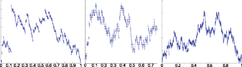
Figure 5: Simulations of $X^{\mathrm{exc}}$ for, respectively, $\theta=1.1,1.5,1.9$.

2.2.1 The Brownian triangulation

Definition 2.4.

The Brownian excursion $\mathbh{e}$ is defined as $X^{\mathrm{exc}}$ for $\theta=2$. For $u,v\in[0,1]$ we set $u\stackrel{{\scriptstyle\mathbh{e}}}{{\thicksim}}v$ if $\mathbh{e}_{u\wedge v}=\mathbh{e}_{u\vee v}=\mathop{\min}_{t\in[u\wedge v,u\vee v]}\mathbh{e}_{t}.$

Note that, with our normalization of $X^{\mathrm{exc}}$, $\mathbh{e}/\sqrt{2}$ is the standard Brownian excursion. It is well known that the local minima of $\mathbh{e}$ are distinct almost surely. In the following, we always discard the set of probability zero where this property fails.

Proposition 2.5 ((Aldous Aldous –Le Gall and Paulin LGP ))

Define $\mathbf{L}(\mathbh{e})$ by

$$\mathbf{L}(\mathbh{e})=\bigcup_{s\stackrel{{\scriptstyle\mathbh{e}}}{{\thicksim}}t}\bigl{[}e^{-2\mathrm{i}\pi s},e^{-2\mathrm{i}\pi t}\bigr{]}.$$

Then $\mathbf{L}(\mathbh{e})$ is a maximal geodesic lamination of $\overline{\mathbb{D}}$ [see Figure 6 for a simulation of $\mathbf{L}(\mathbh{e})$].

Remark 2.6.

Both the property that $\mathbf{L}(\mathbh{e})$ is a lamination and its maximality property are related to the fact that local minima of $\mathbh{e}$ are distinct. The connected components of $\overline{\mathbb{D}}\setminus\mathbf{L}(\mathbh{e})$ are open triangles whose vertices belong to $\mathbb{S}_{1}$. For this reason we call $\mathbf{L}(\mathbh{e})$ the Brownian triangulation. Notice also that $\mathbb{S}_{1}\subset\mathbf{L}(\mathbh{e})$.

2.2.2 The $\theta$-stable lamination

Here, $\theta\in(1,2)$ so that the $\theta$-stable Lévy process $X$ is not continuous. In the beginning of this section we fix $Z\in\mathbb{D}([0,1],\mathbb{R})$ such that $Z_{0}=Z_{1}=0$, $\Delta Z_{s}\geq 0$ for $s\in(0,1]$ and $Z_{s}>0$ for $s\in(0,1)$. We then consider the case when $Z=X^{\mathrm{exc}}$ is the normalized excursion of the $\theta$-stable Lévy process $X$.

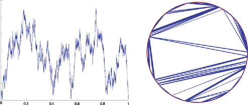
Figure 6: A Brownian excursion $\mathbh{e}$ and the associated triangulation $\mathbf{L}(\mathbh{e})$.

Definition 2.7.

For $0\leq s<t\leq 1$, we set $s\mathop{\simeq}^{Z}t$ if and only if $t=\inf\{u>s;Z_{u}\leq Z_{s-}\}$ (where $Z_{0-}=0$ by definition). For $0\leq t<s\leq 1$, we set $s\mathop{\simeq}^{Z}t$ if and only if $t\mathop{\simeq}^{Z}s$. Finally, we set $s\mathop{\simeq}^{Z}s$ for every $s\in[0,1]$.

Note that $\mathop{\simeq}^{Z}$ is not necessarily an equivalence relation. For example, if $0<r<s<t<1$ are such that $\Delta Z_{r}=0$, $Z_{r}=Z_{s}=Z_{t}$ and $Z_{u}>Z_{r}$ for $u\in(r,s)\cup(s,t)$, then $r\mathop{\simeq}^{Z}s$ and $s\mathop{\simeq}^{Z}t$, but we do not have $r\mathop{\simeq}^{Z}t$.

Remark 2.8.

If $s\mathop{\simeq}^{Z}t$ and $s<t$, then $Z_{s-}=Z_{t}$ and $Z_{r}>Z_{s-}$ for $r\in(s,t)$.

Proposition 2.9

We say that $Z$ attains a local minimum at $t\in(0,1)$ if there exists $\eta>0$ such that $\inf_{[t-\eta,t+\eta]}Z=Z_{t}$. Suppose that $Z$ satisfies the following four assumptions: [(H1)]

If $0\leq s<t\leq 1$, there exists at most one value $r\in(s,t)$ such that $Z_{r}=\inf_{[s,t]}Z$ (we say that local minima of $Z$ are distinct);

If $t\in(0,1)$ is such that $\Delta Z_{t}>0$, then $\inf_{[t,t+\varepsilon]}Z<Z_{t}$ for all $0<\varepsilon\leq 1-t$;

If $t\in(0,1)$ is such that $\Delta Z_{t}>0$, then $\inf_{[t-\varepsilon,t]}Z<Z_{t-}$ for all $0<\varepsilon\leq t$;

Suppose that $Z$ attains a local minimum at $t\in(0,1)$ [in particular, $\Delta Z_{t}=0$ by (H3)]. Let $s=\sup\{r\in[0,t];Z_{r}<Z_{t}\}$. Then $\Delta Z_{s}>0$ and $Z_{s-}<Z_{t}$. Note that then $Z_{s}>Z_{t}$ by (H2). Then the set

$$L(Z):=\bigcup_{s\mathop{\simeq}^{Z}t}\bigl{[}e^{-2\mathrm{i}\pi s},e^{-2\mathrm{i}\pi t}\bigr{]}$$

is a geodesic lamination of $\overline{\mathbb{D}}$, called the lamination coded by the càdlàg function $Z$.

Notice that $\mathbb{S}_{1}\subset L(Z)$ since $s\mathop{\simeq}^{Z}s$ for every $s\in[0,1]$.

It easily follows from Remark 2.8 that the chords appearing in the definition of $L(Z)$ are noncrossing. We have to prove that $L(Z)$ is closed. To this end, it is enough to verify that the relation $\mathop{\simeq}^{Z}$ is closed, in the sense that its graph is a closed subset of $[0,1]^{2}$. Consider two sequences $(s_{n}),(t_{n})$ of reals such that $0\leq s_{n}<t_{n}\leq 1$, $s_{n}\mathop{\simeq}^{Z}t_{n}$ and the pairs $(s_{n},t_{n})$ converge to $(s,t)$. We need to verify that $s\mathop{\simeq}^{Z}t$. Clearly, $s\leq t$ and we can assume that $s<t$ since $\mathbb{S}_{1}\subset L(Z)$.

The property $s_{n}\mathop{\simeq}^{Z}t_{n}$ implies that $Z_{r}\geq Z_{t_{n}}$ for every $r\in(s_{n},t_{n})$. By passing to the limit $n\rightarrow\infty$, we get $Z_{r}\geq Z_{t-}$ for every $r\in(s,t)$. If $\Delta Z_{t}>0$, this contradicts (H3). So we can assume that $\Delta Z_{t}=0$, implying that the sequence $(Z_{t_{n}})$ converges to $Z_{t}$ as $n\rightarrow\infty$.

Case 1. Assume that $\Delta Z_{s}>0$ and thus $s>0$. By (H2) and right-continuity, we can find $\eta>0$ such that $\eta<(t-s)/2$ and

$$\inf_{[s,s+\eta)}Z>\inf_{[s+\eta,(s+t)/2]}Z.$$

It follows from (H3) that the infimum of $Z$ over a compact interval is achieved at some point of this interval. Hence, we may take $r_{0}\in[s+\eta,(s+t)/2]$ such that $Z_{r_{0}}=\inf_{[s+\eta,(s+t)/2]}Z$. If $s<s_{n}$ for infinitely many $n$, we can find infinitely many values of $n$ for which $s<s_{n}<s+\eta\leq r_{0}<t_{n}$. For those values of $n$, $r_{0}\in(s_{n},t_{n})$ and $Z_{r_{0}}<Z_{s_{n}-}$, which contradicts Remark 2.8. We can thus suppose that $s_{n}\leq s$ for every sufficiently large $n$. Consequently, $(Z_{s_{n}-})$ converges to $Z_{s-}$ as $n$ tends to infinity. Since $Z_{s_{n}-}=Z_{t_{n}}$ for all $n$, it follows that $Z_{t}=Z_{s-}$. Recall that $Z_{r}\geq Z_{t}$ for $r\in(s,t)$. We now demonstrate by contradiction that, in fact, $Z_{r}>Z_{t}$ for all $r\in(s,t)$. Suppose that there exists $r_{1}\in(s,t)$ such that $Z_{r_{1}}=Z_{t}$. Notice that $Z$ then attains a local minimum at $r_{1}$. Property (H3) ensures that

$$s=\sup\bigl{\{}u\in[0,r_{1}];Z_{u}<Z_{r_{1}}\bigr{\}},$$

and the fact that $Z_{s-}=Z_{t}=Z_{r_{1}}$ contradicts (H4). We conclude that $Z_{r}>Z_{s-}$ for every $r\in(s,t)$. Therefore, $t=\inf\{u>s;Z_{u}\leq Z_{s-}\}$. This implies that $s\mathop{\simeq}^{Z}t$, as desired.

Case 2. Assume that $\Delta Z_{s}=0$. In this case, $(Z_{s_{n}})$ converges to $Z_{s}$ as $n$ tends to infinity. Since $Z_{s_{n}-}=Z_{t_{n}}$ for all $n$, it follows that $Z_{s}=Z_{t}$. We also know that $Z_{r}\geq Z_{s}$ for $r\in(s,t)$. If $s=0$, we necessarily have $t=1$ and the fact that $Z$ is positive on $(0,1)$ implies $0\mathop{\simeq}^{Z}1$. We thus suppose that $s>0$. Argue by contradiction and suppose that there exists $r_{1}\in(s,t)$ such that $Z_{r_{1}}=Z_{t}$. Then $r_{1}$ is a local minimum of $Z$. If $\inf_{[s-\varepsilon,s]}Z<Z_{s}$ for every $\varepsilon\in(0,s]$, then $s=\sup\{u\in[0,r_{1}];Z_{u}<Z_{r_{1}}\}$. By (H4), $s$ must be a jump time of $Z$, which is a contradiction. If $\inf_{[s-\varepsilon,s]}Z\geq Z_{s}$ for some $\varepsilon\in(0,s]$, this means that $s$ is a local minimum of $Z$. Since $Z_{s}=Z_{r_{1}}$, this contradicts (H1). We conclude that $Z_{r}>Z_{t}$ for $r\in(s,t)$. This implies that $s\mathop{\simeq}^{Z}t$.

Let (H0) be the property: $\{s\in[0,1];\Delta Z_{s}\neq 0\}$ is dense in $[0,1]$.

Proposition 2.10

Let $1<\theta<2$. With probability one, the normalized excursion $X^{\mathrm{exc}}$ of the $\theta$-stable Lévy process satisfies the assumptions (H0), (H1), (H2), (H3) and (H4).

It is sufficient to prove that properties analogous to (H0)–(H4) hold for the Lévy process $X$. The case of (H0) is clear. (H1) and (H2) are consequences of the (strong) Markov property of $X$ and the fact that $0$ is regular for $(-\infty,0)$ with respect to $X$.

For the remaining properties, we will use the time-reversal property of $X$, which states that if $t>0$ and $\widehat{X}^{(t)}$ is the process defined by $\widehat{X}^{(t)}_{s}=X_{t}-X_{(t-s)-}$ for $0\leq s<t$ and $\widehat{X}^{(t)}_{t}=X_{t}$, then the two processes $(X_{s},0\leq s\leq t)$ and $(\widehat{X}^{(t)}_{s},0\leq s\leq t)$ have the same law. For (H3), the time-reversal property of $X$ and the regularity of $0$ for $(0,\infty)$ shows that a.s. for every jump time $s$ of $X$ and every $v\in[0,s)$,

$$\inf_{r\in[v,s]}X_{r}<X_{s-}.$$

We finally prove the analog of (H4) for $X$. By the time-reversal property of $X$, it is sufficient to prove that if $q>0$ is rational and $T=\inf\{t\geq q;X_{t}\geq S_{q}\}$, then $X_{T}>S_{q}\geq X_{T-}$ almost surely. This follows from the Markov property at time $q$ and the fact that for any $a>0$, $X$ jumps a.s. across $a$ at its first passage time above $a$ (see Bertoin , Proposition VIII.8 (ii)).

In the following, we always discard the set of zero probability where one of the properties (H0)–(H4) does not hold.

Definition 2.11.

The $\theta$-stable lamination is defined as the geodesic lamination $L(X^{\mathrm{exc}})$, where $X^{\mathrm{exc}}$ is the normalized excursion of the $\theta$-stable Lévy process.

See Figure 1 for some examples. The following proposition is immediate from the definition of the relation $\mathop{\simeq}^{X^{\mathrm{exc}}}$ and Remark 2.8.

Proposition 2.12

Almost surely, for every choice of $0\leq\alpha<\beta\leq 1$ with $(\alpha,\beta)\neq(0,1)$, we have $\alpha\mathop{\simeq}^{X^{\mathrm{exc}}}\beta$ if and only if one of the following two mutually exclusive cases holds: [(ii)]

$\Delta X^{\mathrm{exc}}_{\alpha}>0$ and $\beta=\inf\{u\geq\alpha;X^{\mathrm{exc}}_{u}=X^{\mathrm{exc}}_{\alpha-}\}$;

$\Delta X^{\mathrm{exc}}_{\alpha}=0$, $X^{\mathrm{exc}}_{\alpha}=X^{\mathrm{exc}}_{\beta}$, and $X^{\mathrm{exc}}_{r}>X^{\mathrm{exc}}_{\alpha}$ for every $r\in(\alpha,\beta)$.

Definition 2.13.

Let $\mathcal{E}_{1}$ be the set of all pairs $(\alpha,\beta)$ where $0\leq\alpha<\beta\leq 1$ satisfy condition (i) in Proposition 2.12.

Proposition 2.14

The following holds almost surely for any pair $(s,t)$ such that $0\leq s<t\leq 1$ and $X^{\mathrm{exc}}_{s}=X^{\mathrm{exc}}_{t}$ and $X^{\mathrm{exc}}_{r}>X^{\mathrm{exc}}_{s}$ for every $r\in(s,t)$. For every $\varepsilon\in(0,(t-s)/2)$, there exist $s^{\prime}\in[s,s+\varepsilon]$ and $t^{\prime}\in[t-\varepsilon,t]$ such that $\Delta X^{\mathrm{exc}}_{s^{\prime}}>0$ and $t^{\prime}=\inf\{u\geq s^{\prime};X^{\mathrm{exc}}_{u}=X^{\mathrm{exc}}_{s^{\prime}-}\}$, so that in particular $(s^{\prime},t^{\prime})\in\mathcal{E}_{1}$.

Let $0\leq s<t\leq 1$ be such that the assumptions in the proposition hold. Take $\varepsilon<(t-s)/4$, then set $m=\inf_{[s+\varepsilon,t-\varepsilon]}X^{\mathrm{exc}}$ and note that $m>X^{\mathrm{exc}}_{s}$ as an easy consequence of (H3). By right-continuity, there exists $\varepsilon^{\prime}$ with $0<\varepsilon^{\prime}<\varepsilon$ such that $\sup_{[s,s+\varepsilon^{\prime}]}X^{\mathrm{exc}}<m$. Let $w\in(s,s+\varepsilon^{\prime})$ be a jump time of $X^{\mathrm{exc}}$, so that, by (H2),

$$\inf_{r\in[w,s+\varepsilon^{\prime}]}X^{\mathrm{exc}}_{r}<X^{\mathrm{exc}}_{w}.$$

We already noticed that the property (H3) implies that the minimum of $X^{\mathrm{exc}}$ over a compact interval is achieved at a point of this interval. Hence, there exists $u\in[w,s+\varepsilon]$ such that $X^{\mathrm{exc}}_{u}=\inf_{[w,s+\varepsilon]}X^{\mathrm{exc}}$. Finally, let $s^{\prime}=\sup\{r\in[s,u];X^{\mathrm{exc}}_{r}<X^{\mathrm{exc}}_{u}\}$. By (H4), we see that $s^{\prime}$ is a jump time. Set $t^{\prime}=\inf\{u>s^{\prime};X^{\mathrm{exc}}_{u}=X^{\mathrm{exc}}_{s^{\prime}-}\}$. By construction, $s\leq s^{\prime}\leq w\leq u\leq s+\varepsilon<t-\varepsilon\leq t^{\prime}\leq t$ and the desired result follows.

Proposition 2.15

We have a.s.

$$L\bigl{(}X^{\mathrm{exc}}\bigr{)}=\overline{\bigcup_{(s,t)\in\mathcal{E}_{1}}\bigl{[}e^{-2\mathrm{i}\pi s},e^{-2\mathrm{i}\pi t}\bigr{]}}.$$

Denote the compact subset of $\overline{\mathbb{D}}$ in the right-hand side by $K$. The fact that $L(X^{\mathrm{exc}})$ is closed implies that $K\subset L(X^{\mathrm{exc}})$. We have to show the reverse inclusion. To this end, let $0\leq u<v\leq 1$ such that $u\mathop{\simeq}^{X^{\mathrm{exc}}}v$ but $(u,v)\notin\mathcal{E}_{1}$. Then condition (ii) in Proposition 2.12 holds for $(\alpha,\beta)=(u,v)$, and it follows from Proposition 2.14 that $(u,v)$ is the limit of a sequence of pairs $(u_{n},v_{n})$ belonging to $\mathcal{E}_{1}$. Since $K$ is closed, we get that $[e^{-2\mathrm{i}\pi u},e^{-2\mathrm{i}\pi v}]\subset K$. Finally, from the fact that $X^{\mathrm{exc}}$ satisfies properties (H0) and (H2), it is easy to verify that in any nontrivial open subinterval of $[0,1]$ we can find a pair $(u,v)$ such that $(u,v)\in\mathcal{E}_{1}$, and it follows that $\mathbb{S}_{1}\subset K$. This completes the proof.

3 Convergence to the stable lamination

In this section we show that the Boltzmann dissections of $P_{n+1}$ considered in Section 1.1 converge in distribution to the stable laminations introduced in the previous section. To this end, we use limit theorems for rescaled Lukasiewicz paths of critical Galton–Watson trees conditioned on their number of leaves, which we obtained in K . We combine these limit theorems with Proposition 1.4 (which states that the dual tree of a Boltzmann dissection is a Galton–Watson tree conditioned on having a given number of leaves) to deduce that the underlying tree structures of large dissections converge. As before, we will deal separately with the case $\theta=2$ and the case $\theta\in(1,2)$. Our goal is to prove the following:

Theorem 3.1

Let $(\mu_{j})_{j\geq 2}$ be a sequence satisfying Assumption $(H_{\theta})$ for some $\theta\in(1,2]$. For every integer $n\geq 2$ such that the definition of $\mathbb{P}^{\mu}_{n}$ makes sense, let $\mathfrak{l}_{n}$ be a random dissection distributed according to $\mathbb{P}^{\mu}_{n}$. Then

$$\mathfrak{l}_{n}\mathop{\longrightarrow}^{(d)}_{n\rightarrow\infty}\cases{\mathbf{L}(\mathbh{e}),&\quad$\mbox{if }\theta=2,$\vspace*{2pt}\cr L\bigl{(}X^{\mathrm{exc}}\bigr{)},&\quad$\mbox{if }\theta\in(1,2),$}$$

where the convergence holds in distribution for the Hausdorff distance on the space of all compact subsets of $\overline{\mathbb{D}}$.

Remarks 3.2.

(i) This theorem generalizes Aldous’ result Aldous , Aldous2 , stating that uniformly distributed triangulations of $P_{n}$ converge to $\mathbf{L}(\mathbh{e})$ as $n\rightarrow\infty$. Indeed, in our setting, uniform triangulations of $P_{n}$ are obtained by taking $\mu_{0}=1/2,\mu_{2}=1/2$ and $\mu_{j}=0$ otherwise. [(iii)]

In CK , it is shown that Theorem 3.1 can be used to study uniformly distributed dissections. More precisely, if one sets $\mu_{0}=2-\sqrt{2}$ and $\mu_{i}=((2-\sqrt{2})/2)^{i-1}$ for every $i\geq 2$, then the Boltzmann probability measure $\mathbb{P}^{\mu}_{n}$ associated to $\mu$ is the uniform probability measure on dissections of $P_{n+1}$.

It would be interesting to understand what happens when the sequence $(\mu_{i})_{i\geq 2}$ does not satisfy $(H_{\theta})$, for instance, if $\sum_{i=2}^{\infty}i\mu_{i}=\infty$. We hope to investigate this in future work.

3.1 Galton–Watson trees conditioned on their number of leaves

Let $\tau\in\mathbb{T}$. Recall our notation $(u(i),0\leq i\leq\zeta(\tau)-1)$ for the vertices of $\tau$ listed in lexicographical order and denote the number of children of $u(j)$ by $k_{j}$. Define $\Lambda_{\tau}(l)$ for every $\ell\in\{0,1,\ldots,\zeta(\tau)\}$ by

$$\Lambda_{\tau}(\ell)=\sum_{0\leq j<\ell}1_{\{k_{j}=0\}}.$$

Note that if $Z=W(\tau)$ is the Lukasiewicz path of $\tau$, $\Lambda_{\tau}$ coincides with $\Lambda$ as defined in Proposition 1.8. Also note that $\Lambda_{\tau}(\zeta(\tau))=\lambda(\tau)$ is the total number of leaves of $\tau$.

Theorem 3.3 ((K ))

Let $(\mu_{j})_{j\geq 2}$ be a sequence of nonnegative real numbers satisfying the assumption $(H_{\theta})$ for some $\theta\in(1,2]$. Put $\mu_{1}=0$ and $\mu_{0}=1-\sum_{j=2}^{\infty}\mu_{j}$, so that $\mu=(\mu_{j})_{j\geq 0}$ is a critical probability measure on $\mathbb{N}$. For every $n\geq 1$ such that $\mathbb{P}_{\mu}[\lambda(\tau)=n]>0$, let $\mathfrak{t}_{n}$ be a random tree distributed according to $\mathbb{P}_{\mu}[\cdot|\lambda(\tau)=n]$. The following two properties hold: [(ii)]

We have

$$\sup_{0\leq t\leq 1}\biggl{|}\frac{\Lambda_{\mathfrak{t}_{n}}(\lfloor\zeta(\mathfrak{t}_{n})t\rfloor)}{n}-t\biggr{|}\mathop{\longrightarrow}^{(\mathbb{P})}_{n\rightarrow\infty}0.$$

There exists a sequence $(B_{k})_{k\geq 1}$ of positive constants converging to $\infty$ such that

$$\biggl{(}\frac{1}{B_{\zeta(\mathfrak{t}_{n})}}W_{\lfloor\zeta(\mathfrak{t}_{n})t\rfloor}(\mathfrak{t}_{n});0\leq t\leq 1\biggr{)}\mathop{\longrightarrow}^{(d)}_{n\rightarrow\infty}\bigl{(}X^{\mathrm{exc}}_{t};0\leq t\leq 1\bigr{)}.$$ (6)

Note that $\Lambda_{\mathfrak{t}_{n}}(\zeta(\mathfrak{t}_{n}))=\lambda(\mathfrak{t}_{n})=n$. In K , Corollary 3.3, it is shown that, for every $0<\eta<1$,

$$\sup_{\eta\leq t\leq 1}\biggl{|}\frac{\Lambda_{\mathfrak{t}_{n}}(\lfloor\zeta(\mathfrak{t}_{n})t\rfloor)}{\zeta(\mathfrak{t}_{n})t}-\mu_{0}\biggr{|}\mathop{\longrightarrow}^{(\mathbb{P})}_{n\rightarrow\infty}0.$$

In particular, this implies that $\zeta(\mathfrak{t}_{n})/n$ converges in probability to $1/\mu_{0}$. Assertion (i) follows from the preceding convergences, noting that, for every $t\in(0,1]$,

$$\frac{\Lambda_{\mathfrak{t}_{n}}(\lfloor\zeta(\mathfrak{t}_{n})t\rfloor)}{n}-t=t\frac{\zeta(\mathfrak{t}_{n})}{n}\biggl{(}\frac{\Lambda_{\mathfrak{t}_{n}}(\lfloor\zeta(\mathfrak{t}_{n})t\rfloor)}{\zeta(\mathfrak{t}_{n})t}-\mu_{0}\biggr{)}+t\biggl{(}\frac{\mu_{0}\zeta(\mathfrak{t}_{n})}{n}-1\biggr{)}.$$

The second assertion is a particular case of K , Theorem 6.1.

3.2 Convergence to the stable lamination

We fix a sequence of nonnegative real numbers $(\mu_{j})_{j\geq 2}$ satisfying Assumption $(H_{\theta})$ for some $\theta\in(1,2]$ and we define $\mu_{0}$ and $\mu_{1}$ as previously. Throughout this section, for every $n\geq 1$ such that $Z_{n}$ defined by (3) is positive (so that $\mathbb{P}^{\mu}_{n}$ is well defined), $\mathfrak{l}_{n}$ stands for a random dissection distributed according to the Boltzmann probability measure $\mathbb{P}^{\mu}_{n}$, and $\mathfrak{t}_{n}$ stands for its dual tree $\phi(\mathfrak{l}_{n})$, which is distributed according to $\mathbb{P}_{\mu}[\cdot|\lambda(\tau)=n]$ by Proposition 1.4. The total progeny of $\mathfrak{t}_{n}$ is denoted by $\zeta_{n}$. The Lukasiewicz path of $\mathfrak{t}_{n}$ is denoted by $W^{n}$ and $u_{0}^{n},u_{1}^{n},\ldots,u_{\zeta_{n}-1}^{n}$ are the vertices of $\mathfrak{t}_{n}$ listed in lexicographical order. Let $(B_{n})_{n\geq 1}$ be a sequence of positive real numbers such that (6) holds. Define the rescaled Lukasiewicz path $X^{n}$ of $\mathfrak{t}_{n}$ by $X^{n}_{t}=\frac{1}{B_{\zeta_{n}}}W^{n}_{\lfloor\zeta_{n}t\rfloor}$ for $0\leq t\leq 1$. By Theorem 3.3 and Skorokhod’s representation theorem (see, e.g., Bill , Theorem 6.7), we may and will assume that the following convergence holds almost surely in the space $\mathbb{R}\otimes\mathbb{D}([0,1],\mathbb{R})$:

$$\biggl{(}\sup_{0\leq t\leq 1}\biggl{|}\frac{\Lambda_{\mathfrak{t}_{n}}(\lfloor\zeta_{n}t\rfloor)}{n+1}-t\biggr{|},X^{n}\biggr{)}\,\mathop{\longrightarrow}_{n\rightarrow\infty}^{a.s.}\,\bigl{(}0,X^{\mathrm{exc}}\bigr{)}.$$ (7)

3.2.1 Convergence to the Brownian triangulation

Here, we suppose that $\theta=2$.

Proposition 3.4

When $n$ tends to infinity, $D(W^{n})\mathop{\rightarrow}\limits^{a.s.}\mathbf{L}(\mathbh{e})$ in the sense of the Hausdorff distance $d_{H}$ between compact subsets of $\overline{\mathbb{D}}$.

We fix $\omega$ in the underlying probability space so that the convergence (7) holds for this value of $\omega$ and we will verify that for this particular value of $\omega$ we have also $D(W^{n})\to\mathbf{L}(\mathbh{e})$. Since the space $(\mathcal{C},d_{H})$ is compact, we may find a random subsequence $(n_{k}(\omega))$ (depending on $\omega$) such that $D(W^{n_{k}})$ converges to a compact subset $K$ of $\overline{\mathbb{D}}$, and we need to verify that $K=\mathbf{L}(\mathbh{e})$. Since $D(W^{n_{k}})$ is a dissection for every $k$, one easily checks that $K$ must be a geodesic lamination of $\overline{\mathbb{D}}$. Since $\mathbf{L}(\mathbh{e})$ is a maximal lamination of $\overline{\mathbb{D}}$, the proof will be complete if we can verify that $\mathbf{L}(\mathbh{e})\subset K$.

So we let $0\leq s<t\leq 1$ be such that $s\stackrel{{\scriptstyle\mathbh{e}}}{{\thicksim}}t$ and we aim at proving that $[e^{-2\mathrm{i}\pi s},e^{-2\mathrm{i}\pi t}]\subset K$. Let $\varepsilon>0$. Simple arguments using the convergence (7) (and the fact that local minima of the Brownian excursion are distinct) show that for every $n$ large enough, we can find integers $i_{n},j_{n}\in\{1,\ldots,\zeta_{n}-1\}$ such that $|i_{n}/\zeta_{n}-s|<\varepsilon$, $|j_{n}/\zeta_{n}-t|<\varepsilon$ and

$$W^{n}_{i_{n}}>W^{n}_{i_{n}-1},\qquad j_{n}=\min\bigl{\{}k>i_{n};W^{n}_{k}<W^{n}_{i_{n}}\bigr{\}}.$$

By Proposition 1.7, $u^{n}_{i_{n}}$ and $u^{n}_{j_{n}}$ are consecutive children of $u^{n}_{i_{n}-1}$. Recalling that $\Lambda_{\mathfrak{t}_{n}}(\zeta(\mathfrak{t}_{n}))=n$, we get from Lemma 1.9 that

$$\biggl{[}\exp\biggl{(}-2\mathrm{i}\pi\frac{\Lambda_{\mathfrak{t}_{n}}(i_{n})}{n+1}\biggr{)},\exp\biggl{(}-2\mathrm{i}\pi\frac{\Lambda_{\mathfrak{t}_{n}}(j_{n})}{n+1}\biggr{)}\biggr{]}\subset D\bigl{(}W^{n}\bigr{)}.$$

To simplify notation, set $s_{n}={\Lambda_{\mathfrak{t}_{n}}(i_{n})}/({n+1})$ and $t_{n}={\Lambda_{\mathfrak{t}_{n}}(j_{n})}/({n+1})$. From the convergence (7), we get $|s_{n}-s|<\varepsilon$ and $|t_{n}-t|<\varepsilon$ for every large enough $n$. In particular, we see that the chord $[e^{-2\mathrm{i}\pi s},e^{-2\mathrm{i}\pi t}]$ lies within distance $2\varepsilon$ from $D(W^{n})$ for every large enough $n$. It follows that the chord $[e^{-2\mathrm{i}\pi s},e^{-2\mathrm{i}\pi t}]$ is within distance $2\varepsilon$ from $K$. Since $\varepsilon>0$ was arbitrary, we get that $[e^{-2\mathrm{i}\pi s},e^{-2\mathrm{i}\pi t}]\subset K$, which completes the proof.

3.2.2 Convergence to the stable lamination when $\theta\neq 2$

We now assume that $\theta\in(1,2)$. Recall that the convergence (7) is assumed to hold a.s.

Proposition 3.5

We have $D(W^{n})\mathop{\rightarrow}\limits^{a.s.}L(X^{\mathrm{exc}})$ as $n\rightarrow\infty$ in the sense of the Hausdorff distance $d_{H}$ between compact subsets of $\overline{\mathbb{D}}$.

We fix $\omega$ in the underlying probability space so that both the conclusion of Proposition 2.15 and the convergence (7) hold for this value of $\omega$ and, furthermore, the path $X^{\mathrm{exc}}(\omega)$ satisfies properties (H0)–(H4). We then consider a subsequence $(n_{k}(\omega))$ such that $D(W^{n_{k}})$ converges to a compact subset $K$ of $\overline{\mathbb{D}}$, and we need to verify that $K={L}(X^{\mathrm{exc}})$. We will first prove that $L(X^{\mathrm{exc}})\subset K$ before proving the reverse inclusion. In both cases, the precise description of $L(X^{\mathrm{exc}})$ as a union of chords will be crucial. Note that $K$ must contain the circle $\mathbb{S}^{1}$ because the dissection $D(W^{n})$ contains the polygon $P_{n+1}$. We stress that the lamination $L(X^{\mathrm{exc}})$ is not maximal, in contrast to the case $\theta=2$. As a consequence, we will have to prove the nontrivial reverse inclusion.

Lemma 3.6

Let $s$ be a jump time of $X^{\mathrm{exc}}$ and $t=\inf\{u>s;X^{\mathrm{exc}}_{u}=X^{\mathrm{exc}}_{s-}\}$. For $\varepsilon\in(0,(t-s)/2)$ small enough, we can choose an integer $n_{0}(\varepsilon)$ such that, for every $n\geq n_{0}(\varepsilon)$, there exists $s_{n}\in(s-\varepsilon,s+\varepsilon)\cap\zeta_{n}^{-1}\mathbb{N}$ such that the following inequalities hold:

$$\inf_{[t-\varepsilon,t+\varepsilon]}X^{n}<X^{n}_{s_{n}-}<\inf_{[s_{n},t-\varepsilon]}X^{n}.$$ (8)

Lemma 3.6 follows from the convergence of $X^{n}$ to $X^{\mathrm{exc}}$ and well-known properties of the Skorokhod topology. We give only the main ideas of the proof and leave the details to the reader. The time $s_{n}$ can be chosen (arbitrarily close to $s$ when $n$ is large) so that $X^{n}_{s_{n}-}$ is close to $X^{\mathrm{exc}}_{s-}$ and $\Delta X^{n}_{s_{n}}$ is close to $\Delta X^{\mathrm{exc}}_{s}$. Then (8) is derived by observing that, for $\varepsilon>0$ small enough,

$$\inf_{[t,t+\varepsilon]}X^{\mathrm{exc}}<X^{\mathrm{exc}}_{t}=X^{\mathrm{exc}}_{s-}<\inf_{[s,t-\varepsilon]}X^{\mathrm{exc}}.$$

Notice that the bound $\inf_{[t,t+\varepsilon]}X^{\mathrm{exc}}<X^{\mathrm{exc}}_{t}$ holds because otherwise $t$ would be a time of local minimum of $X$ and this would contradict (H4).

Lemma 3.7

We have $L(X^{\mathrm{exc}})\subset K$.

Since $K$ is closed, the property of Proposition 2.15 shows that it is enough to verify that $[e^{-2\mathrm{i}\pi\alpha},e^{-2\mathrm{i}\pi\beta}]\subset K$ for every $(\alpha,\beta)\in\mathcal{E}_{1}$. So let $(\alpha,\beta)\in\mathcal{E}_{1}$. Then $\alpha$ is a jump time of $X^{\mathrm{exc}}$ and $\beta=\inf\{u>\alpha;X^{\mathrm{exc}}_{u}=X^{\mathrm{exc}}_{\alpha-}\}$. To show that $[e^{-2\mathrm{i}\pi\alpha},e^{-2\mathrm{i}\pi\beta}]\subset K$, it is sufficient to show that for every $\varepsilon>0$ and every $n$ sufficiently large we can find $\alpha_{n},\beta_{n}\in[0,1]$ such that $|\alpha_{n}-\alpha|\leq 2\varepsilon,|\beta_{n}-\beta|\leq 2\varepsilon$ and $[e^{-2\mathrm{i}\pi\alpha_{n}},e^{-2\mathrm{i}\pi\beta_{n}}]\subset D(W^{n})$. We fix $\varepsilon>0$. Using Lemma 3.6 with $(s,t)=(\alpha,\beta)$, we can, for every large enough $n$, find $\alpha^{\prime}_{n}\in(\alpha-\varepsilon,\alpha+\varepsilon)\cap\zeta_{n}^{-1}\mathbb{N}$ such that

$$\inf_{[\beta-\varepsilon,\beta+\varepsilon]}X^{n}<X^{n}_{\alpha^{\prime}_{n}-}<\inf_{[\alpha^{\prime}_{n},\beta-\varepsilon]}X^{n}.$$

Then put $\beta^{\prime}_{n}=\inf\{u\geq\alpha^{\prime}_{n};X^{n}_{u}<X^{n}_{\alpha^{\prime}_{n}-}\}$ and note that $|\alpha-\alpha^{\prime}_{n}|\leq\varepsilon$, $|\beta-\beta^{\prime}_{n}|\leq\varepsilon$. The time $\zeta_{n}\alpha^{\prime}_{n}$ must correspond to a positive jump of $W^{n}$, and we have also

$$\zeta_{n}\beta^{\prime}_{n}=\inf\bigl{\{}l\geq\zeta_{n}\alpha^{\prime}_{n};W^{n}_{l}=W^{n}_{\zeta_{n}\alpha^{\prime}_{n}}-\bigl{(}W^{n}_{\zeta_{n}\alpha^{\prime}_{n}}-W^{n}_{\zeta_{n}\alpha^{\prime}_{n}-1}+1\bigr{)}\bigr{\}}.$$

Using formula (5) and recalling that $\Lambda_{\mathfrak{t}_{n}}$ coincides with the process $\Lambda$ of Proposition 1.8 if $Z=W^{n}$, we get from Lemma 1.9 that

$$\biggl{[}\exp\biggl{(}-2\mathrm{i}\pi\frac{\Lambda_{\mathfrak{t}_{n}}(\zeta_{n}\alpha^{\prime}_{n})}{n+1}\biggr{)},\exp\biggl{(}-2\mathrm{i}\pi\frac{\Lambda_{\mathfrak{t}_{n}}(\zeta_{n}\beta^{\prime}_{n})}{n+1}\biggr{)}\biggr{]}\subset D\bigl{(}W^{n}\bigr{)}.$$

If we set $\alpha_{n}=(n+1)^{-1}\Lambda_{\mathfrak{t}_{n}}(\zeta_{n}\alpha^{\prime}_{n})$ and $\beta_{n}=(n+1)^{-1}\Lambda_{\mathfrak{t}_{n}}(\zeta_{n}\beta^{\prime}_{n})$, the convergence (7) shows that $\alpha_{n}$ and $\beta_{n}$ satisfy $|\alpha_{n}-\alpha|\leq 2\varepsilon$ and $|\beta_{n}-\beta|\leq 2\varepsilon$ for all sufficiently large $n$, thus giving the desired result.

We now prove the reverse inclusion.

Lemma 3.8

We have $K\subset L(X^{\mathrm{exc}})$.

Recall that $D(W^{n_{k}})$ converges to $K$ in the Hausdorff sense. By the formula of Proposition 1.8, we can write

$$D\bigl{(}W^{n_{k}}\bigr{)}=\bigcup_{(u,v)\in\mathcal{E}_{(n_{k})}}\bigl{[}e^{-2\mathrm{i}\pi u},e^{-2\mathrm{i}\pi v}\bigr{]},$$

where $\mathcal{E}_{(n_{k})}$ is a (finite) symmetric subset of $[0,1]^{2}$. By extracting a subsequence if necessary, we may assume that $\mathcal{E}_{(n_{k})}\rightarrow\mathcal{E}_{\infty}$ in the Hausdorff sense as $k\rightarrow\infty$, where $\mathcal{E}_{\infty}$ is a symmetric closed subset of $[0,1]^{2}$. It is easy to verify that

$$K=\bigcup_{(u,v)\in\mathcal{E}_{\infty}}\bigl{[}e^{-2\mathrm{i}\pi u},e^{-2\mathrm{i}\pi v}\bigr{]}.$$

The proof of the inclusion $K\subset L(X^{\mathrm{exc}})$ then reduces to checking that if $u,v\in\mathcal{E}_{\infty}$ with $u<v$, we have $u\mathop{\simeq}^{X^{\mathrm{exc}}}v$.

So fix $u,v\in\mathcal{E}_{\infty}$ such that $u<v$. Then the pair $(u,v)$ is the limit of a sequence $(u_{k},v_{k})$ with $(u_{k},v_{k})\in\mathcal{E}_{(n_{k})}$ for every $k$. From Proposition 1.8, we can find integers $l_{n_{k}}<m_{n_{k}}$ in $\{0,1,\ldots,\zeta_{n_{k}}\}$ such that

$$u=\lim_{k\to\infty}\frac{\Lambda_{\mathfrak{t}_{n_{k}}}(l_{n_{k}})}{n_{k}+1},\qquad v=\lim_{k\to\infty}\frac{\Lambda_{\mathfrak{t}_{n_{k}}}(m_{n_{k}})}{n_{k}+1}$$

and

$$m_{n_{k}}=\inf\bigl{\{}i\geq l_{n_{k}};W^{n_{k}}_{i}=W^{n_{k}}_{l_{n_{k}}}-1\bigr{\}}.$$ (9)

By (7), we have also

$$u=\lim_{k\rightarrow\infty}\frac{l_{n_{k}}}{\zeta_{n_{k}}},\qquad v=\lim_{k\rightarrow\infty}\frac{m_{n_{k}}}{\zeta_{n_{k}}}.$$ (10)

From (9), we have $W^{n_{k}}_{i}\geq W^{n_{k}}_{m_{n_{k}}}$ for every $i\in[l_{n_{k}},m_{n_{k}}]$. Thus, using the convergence of $X^{n}$ to $X^{\mathrm{exc}}$ and (10),

$$X^{\mathrm{exc}}_{s}\geq X^{\mathrm{exc}}_{v-}\qquad\mathrm{for\ every}\ s\in(u,v).$$ (11)

From property (H3) this implies that $X^{\mathrm{exc}}_{v}=X^{\mathrm{exc}}_{v-}$, and then $(B_{\zeta_{n_{k}}})^{-1}W^{n_{k}}_{m_{n_{k}}}=X^{n_{k}}_{m_{n_{k}}/\zeta_{n_{k}}}$ must converge to $X^{\mathrm{exc}}_{v}$. Note that $X^{\mathrm{exc}}_{u-}$ and $X^{\mathrm{exc}}_{u}$ are the only possible accumulation points for the sequence $(B_{\zeta_{n_{k}}})^{-1}W^{n_{k}}_{l_{n_{k}}}=X^{n_{k}}_{l_{n_{k}}/\zeta_{n_{k}}}$. Now consider two cases:

[$-$]

If $X^{\mathrm{exc}}_{u}=X^{\mathrm{exc}}_{u-}$, then $(B_{\zeta_{n_{k}}})^{-1}W^{n_{k}}_{l_{n_{k}}}=X^{n_{k}}_{l_{n_{k}}/\zeta_{n_{k}}}$ converges to $X^{\mathrm{exc}}_{u}$ and, using (9), we get that $X^{\mathrm{exc}}_{u}=X^{\mathrm{exc}}_{v}$. It follows that $X^{\mathrm{exc}}_{s}>X^{\mathrm{exc}}_{v}$ for every $s\in(u,v)$, because otherwise this would contradict (H1) or (H4). Clearly, we obtain $u\mathop{\simeq}^{X^{\mathrm{exc}}}v$.

If $X^{\mathrm{exc}}_{u}>X^{\mathrm{exc}}_{u-}$, then we must have $X^{n_{k}}_{l_{n_{k}}/\zeta_{n_{k}}}\rightarrow X^{\mathrm{exc}}_{u-}$ [otherwise (9) would give $X^{\mathrm{exc}}_{u}=X^{\mathrm{exc}}_{v}$, and (11) would contradict (H2)]. Then (9) gives $X^{\mathrm{exc}}_{v}=X^{\mathrm{exc}}_{u-}$. The inequality (11) can then be reinforced in $X^{\mathrm{exc}}_{s}>X^{\mathrm{exc}}_{v}=X^{\mathrm{exc}}_{u-}$ for every $s\in(u,v)$, since otherwise $X^{\mathrm{exc}}$ would have a local minimum equal to $X^{\mathrm{exc}}_{v}=X^{\mathrm{exc}}_{u-}$ in $(u,v)$, which would contradict (H4). Hence, we also get $u\mathop{\simeq}^{X^{\mathrm{exc}}}v$ in that case. This completes the proof.

Together with Lemmas 3.7, 3.8 completes the proof of Theorem 3.1 in the case $\theta\neq 2$.

3.3 Description of the faces of $L(X^{\mathrm{exc}})$ for $\theta\neq 2$

We still consider the case $1<\theta<2$. By definition, the faces of $L(X^{\mathrm{exc}})$ are the connected components of $\overline{\mathbb{D}}\setminus L(X^{\mathrm{exc}})$. In this section, we study the faces of $L(X^{\mathrm{exc}})$ and we show in particular that, almost surely, every face of $L(X^{\mathrm{exc}})$ is bounded by infinitely many chords (in contrast to the case $\theta=2$ where all faces are triangles).

Lemma 3.9

Almost surely, for every face $U$ of $L(X^{\mathrm{exc}})$, if $\Gamma=\mathbb{S}_{1}\cap\overline{U}$ denotes the part of the boundary of $U$ lying on the circle, then: [(iii)]

$U$ is a convex open set;

$\Gamma$ is not a singleton;

$1\notin\Gamma$.

Assertions (i) and (ii) hold for any geodesic lamination of $\overline{\mathbb{D}}$, and we leave the proof to the reader. To get (iii), fix $\varepsilon>0$ and note that by Proposition 2.14 we can find $s\in(0,\varepsilon]$ and $t\in[1-\varepsilon,1)$ such that the chord $[e^{-2\mathrm{i}\pi s},e^{-2\mathrm{i}\pi t}]$ is contained in $L(X^{\mathrm{exc}})$. It follows that $1$ cannot belong to the boundary of a connected component of $\overline{\mathbb{D}}\setminus L(X^{\mathrm{exc}})$.

For distinct $s,t\in(0,1)$, we denote by $\mathbb{H}^{s}_{t}$ the open half-plane bounded by the line containing $e^{-2\mathrm{i}\pi s}$ and $e^{-2\mathrm{i}\pi t}$ and such that $1\notin\mathbb{H}^{s}_{t}$. We write $\widetilde{\mathbb{H}}^{s}_{t}$ for the other open half-plane bounded by the same line.

Proposition 3.10

Let $s$ be a jump time of $X^{\mathrm{exc}}$ and $t=\inf\{u>s;X^{\mathrm{exc}}_{u}=X^{\mathrm{exc}}_{s-}\}$. There exists a unique face $U$ of $L(X^{\mathrm{exc}})$ contained in $\mathbb{H}^{s}_{t}$ and whose closure $\overline{U}$ contains the chord $[e^{-2\mathrm{i}\pi s},e^{-2\mathrm{i}\pi t}]$. The face $U$ is called the face associated to $s$. The mapping $s\mapsto U$ is a one-to-one correspondence between jump times of $X^{\mathrm{exc}}$ and faces of $L(X^{\mathrm{exc}})$.

We start by giving a description of the face associated to $s$. Let $(\alpha_{i},\beta_{i})_{i\geq 1}$ be defined by

$$\bigl{\{}(\alpha_{i},\beta_{i});i\geq 1\bigr{\}} = \Bigl{\{}(\alpha,\beta);s\leq\alpha<\beta\leq t,X_{\alpha}=X_{\beta}=\inf_{[s,\alpha]}X\mbox{ and }X^{\mathrm{exc}}_{r}>X^{\mathrm{exc}}_{\alpha}$$

$$\hskip 202.0pt\mbox{for }r\in(\alpha,\beta)\Bigr{\}},$$

where the pairs $(\alpha_{i},\beta_{i})$ are listed in such a way that $\beta_{i}-\alpha_{i}>\beta_{j}-\alpha_{j}$ for $i<j$. The intervals $(\alpha_{i},\beta_{i})$ are exactly the excursion intervals of $(X_{r}-I^{s}_{r})_{s\leq r\leq t}$ away from $0$. Note that $\alpha_{i}\mathop{\simeq}^{X^{\mathrm{exc}}}\beta_{i}$ by Proposition 2.12, and that the intervals $(\alpha_{i},\beta_{i})$, $i\geq 1$ are disjoint. Furthermore, the fact that (H3) holds for $X^{\mathrm{exc}}$ shows that the times $\alpha_{i}$, $i\geq 1$ are not jump times of $X^{\mathrm{exc}}$.

For every $n\geq 1$, let $V_{n}$ be the convex open polygon whose vertices are

$$\bigl{\{}e^{-2\mathrm{i}\pi s},e^{-2\mathrm{i}\pi t}\bigr{\}}\cup\bigcup_{i=1}^{n}\bigl{\{}e^{-2\mathrm{i}\pi\alpha_{i}},e^{-2\mathrm{i}\pi\beta_{i}}\bigr{\}}.$$

Observe that $V_{n}\subset V_{n+1}$. We finally set

$$V=\bigcup_{n\geq 1}V_{n},$$

which is a convex open set. It is clear that $V$ is contained in the open half-plane $\mathbb{H}^{s}_{t}$ and that $\overline{V}$ contains $[e^{-2\mathrm{i}\pi s},e^{-2\mathrm{i}\pi t}]$. To prove that $V$ is a connected component of $\overline{\mathbb{D}}\setminus L(X^{\mathrm{exc}})$, we proceed in two steps. We first prove that $V\subset\overline{\mathbb{D}}\setminus L(X^{\mathrm{exc}})$ and then that $V$ is a maximal connected open subset of $\overline{\mathbb{D}}\setminus L(X^{\mathrm{exc}})$.

Let us prove that $V\subset\overline{\mathbb{D}}\setminus L(X^{\mathrm{exc}})$. Argue by contradiction and suppose that there exist $P\in L(X^{\mathrm{exc}})$ and $N\geq 1$ such that $P\in V_{N}$. By the definition of $L(X^{\mathrm{exc}})$, there exist $0\leq u\leq v<1$ such that $u\mathop{\simeq}^{X^{\mathrm{exc}}}v$ and $P\in[e^{-2\mathrm{i}\pi u},e^{-2\mathrm{i}\pi v}]$. Since $V$ is contained in the open half-plane $\mathbb{H}^{s}_{t}$, we must have $s\leq u<v\leq t$. Let us first show that $s<u$. If $s=u$, the definition of $\mathop{\simeq}^{X^{\mathrm{exc}}}$ implies that $v=\inf\{r>s;X^{\mathrm{exc}}_{r}=X^{\mathrm{exc}}_{s-}\}=t$. Consequently, $P\in[e^{-2\mathrm{i}\pi s},e^{-2\mathrm{i}\pi t}]$, contradicting the fact that $P\in V_{N}$. We thus have $s<u$. Since $P\in V_{N}$ and since for every $j\in\{1,\ldots,N\}$ the chord $[e^{-2\mathrm{i}\pi\alpha_{j}},e^{-2\mathrm{i}\pi\beta_{j}}]$ does not cross the chord $[e^{-2\mathrm{i}\pi u},e^{-2\mathrm{i}\pi v}]$, a simple argument shows that there exists $1\leq i\leq N$ such that $u\leq\alpha_{i}<\beta_{i}\leq v$, the case $(u,v)=(\alpha_{i},\beta_{i})$ being excluded. We examine two cases: [$-$]

If $u<\alpha_{i}$, then $X^{\mathrm{exc}}_{u-}>X^{\mathrm{exc}}_{\alpha_{i}}$ because $\inf_{[s,\alpha_{i}]}X^{\mathrm{exc}}=X^{\mathrm{exc}}_{\alpha_{i}}$, $\alpha_{i}$ is a local minimum time for $X^{\mathrm{exc}}$ and local minima are almost surely distinct. Since $\alpha_{i}\in[u,v]$ and $u\mathop{\simeq}^{X^{\mathrm{exc}}}v$, this contradicts Remark 2.8.

If $u=\alpha_{i}$, we know that $u$ is not a jump time of $X^{\mathrm{exc}}$ and the property $u\mathop{\simeq}^{X^{\mathrm{exc}}}v$ implies $v=\inf\{r>u;X^{\mathrm{exc}}_{r}\leq X^{\mathrm{exc}}_{\alpha_{i}}\}=\beta_{i}$, which is excluded. In each case, a contradiction occurs. This completes the first step.

Let us then prove that $V$ is a maximal connected open subset of $\overline{\mathbb{D}}\setminus L(X^{\mathrm{exc}})$. To this end, we observe that we have

$$V=\mathbb{H}^{s}_{t}\cap\Biggl{(}\bigcap_{i=1}^{\infty}\widetilde{\mathbb{H}}^{\alpha_{i}}_{\beta_{i}}\Biggr{)}\cap\mathbb{D}.$$

The fact that $V$ is contained in the set in the right-hand side is immediate from our construction, and the reverse inclusion is also easy. Set $R=(\mathbb{H}^{s}_{t})^{c}\cap\overline{\mathbb{D}}$ and $R_{i}=(\widetilde{\mathbb{H}}^{\alpha_{i}}_{\beta_{i}})^{c}\cap\overline{\mathbb{D}}$ for $i\geq 1$. It follows that

$$\overline{\mathbb{D}}\setminus V=\mathbb{S}_{1}\cup R\cup\Biggl{(}\bigcup_{i=1}^{\infty}R_{i}\Biggr{)}.$$ (12)

This implies that the boundary of $V$ is contained in $L(X^{\mathrm{exc}})$, and it follows that $V$ is a maximal connected open subset of $\overline{\mathbb{D}}\setminus L(X^{\mathrm{exc}})$. From the preceding formula for $\overline{\mathbb{D}}\setminus V$, it is also clear that the boundary of $V$ contains the chord $[e^{-2\mathrm{i}\pi s},e^{-2\mathrm{i}\pi t}]$, as well as all chords $[e^{-2\mathrm{i}\pi\alpha_{i}},e^{-2\mathrm{i}\pi b_{i}}]$, and we have obtained the existence of the face associated to $s$. The uniqueness of this face is obvious for geometric reasons.

We still have to prove the last assertion of the proposition. Let $U$ be a face of $L(X^{\mathrm{exc}})$. We need to verify that $U$ is the face associated to a certain jump time of $X^{\mathrm{exc}}$. To this end, let $\Gamma=\mathbb{S}_{1}\cap\overline{U}$ be the part of the boundary of $U$ lying on the circle and set:

$$s=\inf\bigl{\{}u\geq 0;e^{-2\mathrm{i}\pi u}\in\Gamma\bigr{\}},\qquad t=\sup\bigl{\{}0\leq u\leq 1;e^{-2\mathrm{i}\pi u}\in\Gamma\bigr{\}}.$$

By Lemma 3.9(iii), we have $0<s<t<1$. By the compactness of $L(X^{\mathrm{exc}})$ and a convexity argument, it is easy to verify that $[e^{-2\mathrm{i}\pi s},e^{-2\mathrm{i}\pi t}]\subset L(X^{\mathrm{exc}})$. We then claim that $s$ is a jump time of $X^{\mathrm{exc}}$. If not, by Proposition 2.12, this means that $X^{\mathrm{exc}}_{s}=X^{\mathrm{exc}}_{t}$ and $X^{\mathrm{exc}}_{u}>X^{\mathrm{exc}}_{s}$ for $u\in(s,t)$. But then Proposition 2.14 could be used to produce a chord of $L(X^{\mathrm{exc}})$ partitioning $U$ into two disjoint open sets, which is impossible. So $s$ is a jump time of $X^{\mathrm{exc}}$ and we then know that $t=\inf\{u>s;X^{\mathrm{exc}}_{u}=X^{\mathrm{exc}}_{s-}\}$. Let $V$ be the face associated to $s$. To prove that $U=V$, it is sufficient to show that $U\cap V\neq\varnothing$. This follows from simple geometric considerations. This completes the proof.

4 The stable lamination coded by a continuous function

The definitions of the limiting random laminations $\mathbf{L}(\mathbh{e})$ and $L(X^{\mathrm{exc}})$ that appear in our main result Theorem 3.1 for $\theta=2$ and $\theta\neq 2$ were somewhat different. The goal of this section is to unify these two cases by explaining how $L(X^{\mathrm{exc}})$ (for $\theta\neq 2$) can also be constructed from a random continuous function. This will allow us to make the connection between our stable laminations and the so-called stable trees, which were studied in particular in DuquesneLG , DuquesneLG-fractal , in the same way as the Brownian triangulation is connected to the Brownian CRT Aldous2 , and this will also be useful when we calculate the Hausdorff dimension of $L(X^{\mathrm{exc}})$. The relevant random function, called the height process in continuous time, was introduced in LeJan and studied in great detail in DuquesneLG .

In this section, $X$ is the strictly stable spectrally positive Lévy of index $\theta$, as defined in Section 2.1 and $1<\theta<2$.

4.1 The height process

The continuous-time height process associated with $X$ can be defined by the following approximation formula. For every $t\geq 0$,

$$H_{t}=\lim_{\varepsilon\rightarrow 0}\frac{1}{\varepsilon}\int_{0}^{t}ds\mathbh{1}_{\{X_{s}\leq I^{s}_{t}+\varepsilon\}},$$

where the convergence holds in probability. The process $(H_{t})_{t\geq 0}$ has a continuous modification, which we consider from now on.

A very useful ingredient in the study of the height process is the so-called exploration process $(\rho_{t})_{t\geq 0}$, which is a strong Markov process taking values in the space $M_{f}(\mathbb{R}_{+})$ of all finite measures on $\mathbb{R}_{+}$. For every $t\geq 0$, $\rho_{t}$ is defined by

$$\langle\rho_{t},f\rangle=\int_{[0,t]}d_{s}I^{s}_{t}f({H_{s}})$$ (13)

for every measurable function $f\dvtx\mathbb{R}_{+}\rightarrow\mathbb{R}_{+}$. Here the notation $d_{s}I^{s}_{t}$ refers to the integration with respect to the nondecreasing function $s\rightarrow I^{s}_{t}$ (recall the definition of $I^{s}_{t}$ in Section 2.1). Note, in particular, that $\langle\rho_{t},1\rangle=X_{t}-I_{t}$. The process $(\rho_{t})_{t\geq 0}$ enjoys the following two important properties DuquesneLG , Lemma 1.2.2: [(ii)]

Almost surely for every $t\geq 0$, $\rho_{t}(\{0\})=0$ and $\operatorname{supp}(\rho_{t})=[0,H_{t}]$ [here and later $\operatorname{supp}(\mu)$ denotes the topological support of $\mu\in M_{f}(\mathbb{R}_{+})$, with the convention that $\operatorname{supp}(0)=\{0\}$].

Almost surely $\{t\geq 0;H_{t}=0\}=\{t\geq 0;\rho_{t}=0\}=\{t\geq 0;X_{t}=I_{t}\}$. In addition to (i), one can prove that, for every fixed $t\geq 0$, $\rho_{t}(\{H_{t}\})=0$ almost surely. This follows from formula (17) in DuquesneLG . Moreover, almost surely for every jump time $s$ of $X$, $\rho_{s}(\{H_{s}\})=\Delta X_{s}$ (see formula (19) in DuquesneLG ).

We will need another important property of the exploration process. To state this property, we need to introduce some notation. If $\mu\in M_{f}(\mathbb{R}_{+})$ and $\alpha\geq 0$, the “killed” measure $k_{\alpha}\mu$ is the unique element of $M_{f}(\mathbb{R}_{+})$ such that, for every $t\geq 0$,

$$k_{\alpha}\mu\bigl{(}[0,t]\bigr{)}=\mu\bigl{(}[0,t]\bigr{)}\wedge\bigl{(}\mu(\mathbb{R}_{+})-\alpha\bigr{)}^{+}.$$

Suppose that $\mu\in M_{f}(\mathbb{R}_{+})$ has compact support and set $h(\mu)=\sup(\operatorname{supp}(\mu))$. Then if $\nu\in M_{f}(\mathbb{R}_{+})$, the concatenation $[\mu,\nu]\in M_{f}(\mathbb{R}_{+})$ is defined by

$$\bigl{\langle}[\mu,\nu],f\bigr{\rangle}=\langle\mu,f\rangle+\int\nu(dt)f\bigl{(}h(\mu)+t\bigr{)}.$$

Let $T$ be a stopping time of the filtration of $X$ and let $X_{t}^{(T)}=X_{T+t}-X_{T}$ for every $t\geq 0$. Recall that $(X^{(T)}_{t})_{t\geq 0}$ has the same distribution as $(X_{t})_{t\geq 0}$ by the strong Markov property of $X$. Set $I^{(T)}_{t}=\inf_{s\leq t}X^{(T)}_{s}$ for every $t\geq 0$, and let $(H_{t}^{(T)})_{t\geq 0}$ and $(\rho^{(T)}_{t})_{t\geq 0}$ be, respectively, the height process and the exploration process associated with $X^{(T)}$. According to formula (20) in DuquesneLG , we have almost surely for every $t\geq 0$,

$$\rho_{T+t}=\bigl{[}k_{-I^{(T)}_{t}}\rho_{T},\rho_{t}^{(T)}\bigr{]}.$$ (14)

It follows that almost surely for every $t\geq 0$,

$$H_{T+t}-\inf_{s\in[T,T+t]}H_{s}=H_{t}^{(T)}$$ (15)

(see DuquesneLG , Lemma 1.4.5, for the case where $T$ is deterministic, but the derivation is the same in the general case).

The following result is a continuous analog of Proposition 1.7.

Proposition 4.1

The following holds almost surely. Let $s\geq 0$ be a jump time of $X$ and $t=\inf\{u>s;X_{u}=X_{s-}\}$. Then: [(iii)]

for every $u\in[s,t]$, $H_{u}\geq H_{s}$ and $H_{u}=H_{s}$ if and only if $X_{u}=\inf_{[s,u]}X$;

for every $\alpha\in[0,s)$, $\inf_{[\alpha,s]}H<H_{s}$;

for every $u\in(t,\infty)$, $\inf_{[s,u]}H<H_{s}$.

Since the set of all jump times can be written as a countable collection of stopping times, it is sufficient to consider the case when $s=S$ is a stopping time, that is, also a jump time of $X$, and $t=T=\inf\{r\geq S;X_{r}=X_{S-}\}$. By preceding observations, we know that $\rho_{S}(\{H_{S}\})=\Delta X_{S}$.

Let us prove (i). From (14) applied to the stopping time $S$, we have $\rho_{S+r}\geq k_{\Delta X_{S}}\rho_{S}$ for every $r\in[0,T-S]$ and, thus,

$$H_{S+r}=\sup(\operatorname{supp}\rho_{S+r})\geq\sup(\operatorname{supp}k_{\Delta X_{S}}\rho_{S})=H_{S}.$$

Furthermore, for the same values of $r$, (14) shows that $H_{S+r}=H_{S}$ can only hold if $\rho^{(S)}_{r}=0$, which is equivalent [by (13)] to $X^{(S)}_{r}=I^{(S)}_{r}$. This completes the proof of (i).

To get (ii), we observe that we can always pick a rational $\beta\in(\alpha,S)$ such that $X_{\beta}<X_{S}$. By (15) applied to $T=\beta$,

$$H_{S}-\inf_{r\in[\alpha,S]}H_{r}\geq H_{S}-\inf_{r\in[\beta,S]}H_{r}=H^{(\beta)}_{S-\beta}.$$

Since $X_{S}>X_{\beta}$, we have $\langle\rho^{(\beta)}_{S-\beta},1\rangle\geq X^{(\beta)}_{S-\beta}>0$ and, thus, $H^{(\beta)}_{S-\beta}>0$, completing the proof of (ii).

Finally, for every $\varepsilon>0$ set $T_{\varepsilon}=\inf\{r\geq S;X_{r}\leq X_{S-}-\varepsilon\}$. By (14) we have $\rho_{T_{\varepsilon}}=k_{\Delta X_{s}+\varepsilon}\rho_{S}$ and $H_{T_{\varepsilon}}=\sup(\operatorname{supp}k_{\Delta X_{s}+\varepsilon}\rho_{S})<H_{S}$ because $\rho_{S}(\{H_{S}\})=\Delta X_{S}$. This completes the proof.

The following result will also be useful.

Proposition 4.2

The following holds almost surely for every choice of $0\leq s<t$ such that $H_{s}=H_{t}$ and $H_{u}>H_{s}$ for all $u\in(s,t)$. For every $\varepsilon\in(0,(t-s)/2)$, there exist $s^{\prime}\in(s,s+\varepsilon)$ and $t^{\prime}\in(t-\varepsilon,t)$ such that $s^{\prime}<t^{\prime}$ and: [(ii)]

$H$ does not attain a local minimum at $s^{\prime}$ or at $t^{\prime}$;

$H_{s^{\prime}}=H_{t^{\prime}}=\inf_{[s^{\prime},t^{\prime}]}H$ and there exists $v\in(s^{\prime},t^{\prime})$ such that $H_{v}=H_{s^{\prime}}$.

We can assume that $\varepsilon<(t-s)/4$. Set $m=\inf_{[s+\varepsilon,t-\varepsilon]}H$. By the continuity of $H$, there exists $\varepsilon^{\prime}\in(0,\varepsilon)$ such that $\sup_{[s,s+\varepsilon^{\prime}]}H<m$. Let $u\in(s,s+\varepsilon^{\prime})\cap\mathbb{Q}$. We have

$$\inf_{[u,s+\varepsilon^{\prime}]}H<H_{u}$$

because it easily follows from formula (14) that $\inf_{[q,q+\delta]}H<H_{q}$ for every rational $q>0$ and every $\delta>0$, almost surely (the point is that the measure $\rho_{q}$ gives no mass to $\{H_{q}\}$, so that the supremum of the support of $k_{a}\rho_{q}$ will be strictly smaller than $H_{q}$, for every $a>0$).

Then let $v\in(u,s+\varepsilon^{\prime}]$ be such that $H_{v}=\inf_{[u,s+\varepsilon^{\prime}]}H$. Finally, set $s^{\prime}=\inf\{r\in[s,s+\varepsilon^{\prime}];H_{r}=H_{v}\}$ and $t^{\prime}=\sup\{r\in[s+\varepsilon^{\prime},t];H_{r}=H_{v}\}$ so that $H$ does not attain a local minimum at $s^{\prime}$ or at $t^{\prime}$. By construction and using the continuity of $H$, we have

$$s<s^{\prime}\leq u<v\leq s+\varepsilon<t-\varepsilon<t^{\prime}<t.$$

Since $H_{s^{\prime}}=H_{v}=H_{t^{\prime}}$, the proposition is proved.

4.2 The normalized excursion of the height process

Recall the notation of Section 2.1, where we have constructed the normalized excursion $X^{\mathrm{exc}}$ from the excursion of $X$ straddling $1$.

The normalized excursion of the height process, which is denoted by $H^{\mathrm{exc}}$, is defined as follows. Set $\beta_{\varepsilon}=\theta/(\Gamma(2-\theta)\varepsilon^{\theta-1})$. Using Proposition 2.1, one shows that there exists a continuous process $(H^{\mathrm{exc}}_{t})_{0\leq t\leq 1}$, such that, for every $t$ belonging to a subset of $[0,1]$ of full Lebesgue measure,

$$H_{t}^{\mathrm{exc}}=\lim_{\varepsilon\rightarrow 0}\frac{1}{\beta_{\varepsilon}}\operatorname{Card}\Bigl{\{}u\in[0,t];X^{\mathrm{exc}}_{u-}<\inf_{[u,t]}X^{\mathrm{exc}},\Delta X^{\mathrm{exc}}_{u}>\varepsilon\Bigr{\}}\qquad\mbox{a.s.}$$

See Duquesne , Section 3, for details of the argument. This process $H^{\mathrm{exc}}$ is called the normalized excursion of the height process. The pair $(X^{\mathrm{exc}},H^{\mathrm{exc}})$ can be constructed explicitly from the process $X$ via the formula

$$\quad\bigl{(}X^{\mathrm{exc}}_{t},H^{\mathrm{exc}}_{t}\bigr{)}_{0\leq t\leq 1}=\bigl{(}\zeta_{1}^{-{1}/{\theta}}(X_{\underline{g}_{1}+\zeta_{1}t}-X_{\underline{g}_{1}}),\zeta_{1}^{({1}/{\theta})-1}H_{\underline{g}_{1}+\zeta_{1}t}\bigr{)}_{0\leq t\leq 1},$$ (16)

where we recall the notation $\underline{g}_{1}=\sup\{s\leq 1;X_{s}=I_{s}\}$ and $\zeta_{1}=\underline{g}_{1}-\inf\{s>1;X_{s}=I_{s}\}$.

Remark 4.3.

From formula (16), we see that the results of Propositions 4.1 and 4.2 remain valid if we replace $X$ with $X^{\mathrm{exc}}$ and $H$ with $H^{\mathrm{exc}}$. More precisely, we will use these results in the following form. Almost surely:

1. [(1)]

2. Let $0\leq s\leq 1$ be a jump time of $X^{\mathrm{exc}}$ and $t=\inf\{u>s;X^{\mathrm{exc}}_{u}=X^{\mathrm{exc}}_{s-}\}$. Then for $u\in[s,t]$, $H^{\mathrm{exc}}_{u}\geq H^{\mathrm{exc}}_{s}$, and $H^{\mathrm{exc}}_{u}=H^{\mathrm{exc}}_{s}$ if and only if $X^{\mathrm{exc}}_{u}=\inf_{[s,u]}X^{\mathrm{exc}}$. Moreover, if $0\leq\alpha<s$, then $\inf_{[\alpha,s]}H^{\mathrm{exc}}<H^{\mathrm{exc}}_{s}$, and if $t<u\leq 1$, then $\inf_{[s,u]}H^{\mathrm{exc}}<H^{\mathrm{exc}}_{s}$;

3. For every choice of $0\leq s<t\leq 1$, the conditions $H^{\mathrm{exc}}_{s}=H^{\mathrm{exc}}_{t}$ and $H^{\mathrm{exc}}_{u}>H^{\mathrm{exc}}_{s}$ for all $u\in(s,t)$ imply that for every $\varepsilon>0$ sufficiently small, there exist $s^{\prime}\in(s,s+\varepsilon)$ and $t^{\prime}\in(t-\varepsilon,t)$ such that:

   1. [(ii)]

   2. $H^{\mathrm{exc}}$ does not attain a local minimum at $s^{\prime}$ or at $t^{\prime}$,

   3. $\inf_{[s^{\prime},t^{\prime}]}H^{\mathrm{exc}}=H^{\mathrm{exc}}_{s^{\prime}}=H^{\mathrm{exc}}_{t^{\prime}}$ and there exists $u\in(s^{\prime},t^{\prime})$ such that $H^{\mathrm{exc}}_{u}=H^{\mathrm{exc}}_{s^{\prime}}=H^{\mathrm{exc}}_{t^{\prime}}$.

The main result of Duquesne states that if $\mathfrak{t}_{n}$ is a $GW_{\mu}$ tree conditioned on having total progeny $n$, the discrete height process $(H_{k}(\mathfrak{t}_{n}))_{0\leq k\leq n}$, appropriately rescaled, converges in distribution to $H^{\mathrm{exc}}$. However, we will not use this fact.

4.3 Laminations coded by continuous functions

Let $g\dvtx[0,1]\rightarrow\mathbb{R}_{+}$ be a continuous function such that $g(0)=g(1)=0$. We define a pseudo-distance on $[0,1]$ by

$$d_{g}(s,t)=g(s)-g(t)-2\min_{r\in[s\wedge t,s\vee t]}g(r)$$

for $s,t\in[0,1]$. The associated equivalence relation on $[0,1]$ is defined by setting $s\stackrel{{\scriptstyle g}}{{\thicksim}}t$ if and only if $d_{g}(s,t)=0$ or, equivalently, $g(s)=g(t)=\break\min_{r\in[s\wedge t,s\vee t]}g(r)$ (in the special case $g=\mathbh{e}$, this equivalence relation was already used in Section 2).

The quotient set $T_{g}:=[0,1]/\stackrel{{\scriptstyle g}}{{\thicksim}}$ equipped with the distance $d_{g}$ is an $\mathbb{R}$-tree, called the tree coded by the function $g$. We refer to DuquesneLG-fractal , Evans for more information about $\mathbb{R}$-trees, which are natural generalizations of discrete trees, and their coding by functions.

For $s\in[0,1]$, we let $\operatorname{cl}_{g}(s)$ be the equivalence class of $s$ with respect to the equivalence relation $\stackrel{{\scriptstyle g}}{{\thicksim}}$. Then, for $s,t\in[0,1]$, we set $s\stackrel{{\scriptstyle g}}{{\thickapprox}}t$ if at least one of the following two conditions holds: [$-$]

$s\mathop{\thicksim}\limits^{g}t$ and $g(r)>g(s)$ for every $r\in(s\wedge t,s\vee t)$;

$s\mathop{\thicksim}\limits^{g}t$ and $s\wedge t=\min\operatorname{cl}_{g}(s)$, $s\vee t=\max\operatorname{cl}_{g}(s).$

By CLG , Proposition 2.5, the set

$$\mathbf{L}(g):=\bigcup_{s\stackrel{{\scriptstyle g}}{{\thickapprox}}t}\bigl{[}e^{-2\mathrm{i}\pi s},e^{-2\mathrm{i}\pi t}\bigr{]}$$

is a geodesic lamination of $\overline{\mathbb{D}}$. Note that if $g=\mathbh{e}$, this coincides with the definition in Section 2, thanks to the fact that local minima of $\mathbh{e}$ are distinct.

In what follows we take $g=H^{\mathrm{exc}}$ and write $\thickapprox^{H^{\mathrm{exc}}}$ rather than $\stackrel{{\scriptstyle H^{\mathrm{exc}}}}{{\thickapprox}}$ for notational reasons.

Proposition 4.4

Almost surely, for every real number $u\in[0,1]$ such that $\operatorname{Card}(\operatorname{cl}_{H^{\mathrm{exc}}}(u))\geq 3$, there exists a jump time $\alpha$ of $X^{\mathrm{exc}}$ such that $\alpha\in\operatorname{cl}_{H^{\mathrm{exc}}}(u)$. Conversely, let $\alpha$ be a jump time of $X^{\mathrm{exc}}$ and $\beta=\inf\{r>\alpha;X^{\mathrm{exc}}_{r}=X^{\mathrm{exc}}_{\alpha-}\}$. Then $\operatorname{Card}(\operatorname{cl}_{H^{\mathrm{exc}}}(\alpha))=\infty$, furthermore, $\min\operatorname{cl}_{H^{\mathrm{exc}}}(\alpha)=\alpha$ and $\max\operatorname{cl}_{H^{\mathrm{exc}}}(\alpha)$ $=\beta$, so that, in particular, $\alpha\thickapprox^{H^{\mathrm{exc}}}\beta$.

The first assertion is a consequence of Theorem 4.7 in DuquesneLG-fractal and the discussion following this statement. The fact that $\operatorname{Card}(\operatorname{cl}_{H^{\mathrm{exc}}}(\alpha))=\infty$ if $\alpha$ is a jump time of $X^{\mathrm{exc}}$ follows from DuquesneLG-fractal , Theorem 4.6. Finally, let $\alpha$ be a jump time of $X^{\mathrm{exc}}$ and let $\beta=\inf\{r\geq\alpha;X^{\mathrm{exc}}_{r}=X^{\mathrm{exc}}_{\alpha-}\}$. By the first part of Remark 4.3, we know that $H^{\mathrm{exc}}_{\alpha}=\inf_{[\alpha,\beta]}H^{\mathrm{exc}}=H^{\mathrm{exc}}_{\beta}$ and that for any $\varepsilon>0$,

$$\inf_{[\alpha-\varepsilon,\alpha]}H^{\mathrm{exc}}<H^{\mathrm{exc}}_{\alpha},\qquad\inf_{[\beta,\beta+\varepsilon]}H^{\mathrm{exc}}<H^{\mathrm{exc}}_{\beta}.$$

The desired result follows.

Theorem 4.5

Almost surely, the relations $\mathop{\simeq}^{X^{\mathrm{exc}}}$ and $\mathop{\thickapprox}^{H^{\mathrm{exc}}}$ coincide. In particular,

$$L\bigl{(}X^{\mathrm{exc}}\bigr{)}=\mathbf{L}\bigl{(}H^{\mathrm{exc}}\bigr{)}\qquad\mbox{a.s.}$$

We first observe that both relations $\mathop{\simeq}^{X^{\mathrm{exc}}}$ and $\mathop{\thickapprox}^{H^{\mathrm{exc}}}$ are closed, in the sense that their graphs are closed subsets of $[0,1]^{2}$. In the case of $\mathop{\simeq}^{X^{\mathrm{exc}}}$, this was already observed in the proof of Proposition 2.9. In the case of $\mathop{\thickapprox}^{H^{\mathrm{exc}}}$, this is elementary (see CLG , Section 2.3).

Let $s,t\in[0,1]$ such that $s<t$ and $s\mathop{\simeq}^{X^{\mathrm{exc}}}t$. From Proposition 2.14, we can write the pair $(s,t)$ as the limit of a sequence $(s_{n},t_{n})$ in $\mathcal{E}_{1}$ (of course, if $s$ is a jump time of $X^{\mathrm{exc}}$, we take $s_{n}=s$ and $t_{n}=t$ for every $n$). However, Proposition 4.4 then implies that $s_{n}\thickapprox^{H^{\mathrm{exc}}}t_{n}$, for every $n$, and it follows that $s\thickapprox^{H^{\mathrm{exc}}}t$.

Let us prove the converse. Let $(s,t)$ be such that $0\leq s<t\leq 1$ and $s\mathop{\thickapprox}^{H^{\mathrm{exc}}}t$. If $\operatorname{Card}(\operatorname{cl}_{H^{\mathrm{exc}}}(s))\geq 3$, we must have $s=\min\operatorname{Card}(\operatorname{cl}_{H^{\mathrm{exc}}}(s))$ and $t=\max\operatorname{Card}(\operatorname{cl}_{H^{\mathrm{exc}}}(s))$, so that Proposition 4.4 implies that the pair $(s,t)$ belongs to $\mathcal{E}_{1}$, and, in particular, $s\mathop{\simeq}^{X^{\mathrm{exc}}}t$. If $\operatorname{Card}(\operatorname{cl}_{H^{\mathrm{exc}}}(s))=2$, then the second part of Remark 4.3 shows that $(s,t)$ is the limit of a sequence of pairs $s_{n},t_{n}$ such that $s_{n}\mathop{\thickapprox}^{H^{\mathrm{exc}}}t_{n}$ and $\operatorname{Card}(\operatorname{cl}_{H^{\mathrm{exc}}}(s_{n}))\geq 3$. We have then $s_{n}\mathop{\simeq}^{X^{\mathrm{exc}}}t_{n}$ for every $n$ and $s\mathop{\simeq}^{X^{\mathrm{exc}}}t$ since the relation $\mathop{\simeq}^{X^{\mathrm{exc}}}$ is closed.

Remark 4.6.

In the discrete setting, the definition of the dissection $D(W(\tau))$ via formula (5) uses the times $s^{i}_{1},\ldots,s^{i}_{k_{i}}$, which can be defined either from the Lukasiewicz path of $\tau$ as in Proposition 1.7(i) or from the discrete height process of $\tau$ as in part (ii) of the same proposition. In the continuous setting, we recover these two different points of view in the definition of the $\theta$-stable lamination as $L(X^{\mathrm{exc}})$ or $\mathbf{L}(H^{\mathrm{exc}})$.

5 The Hausdorff dimension of the stable lamination

In this section we determine the Hausdorff dimension of $L(X^{\mathrm{exc}})$ and of some other random sets related to $L(X^{\mathrm{exc}})$. We refer the reader to Mattila for background concerning Hausdorff and Minkowski dimensions.

Theorem 5.1

Fix $\theta\in(1,2]$. Let $L(X^{\mathrm{exc}})$ be the random lamination coded by the normalized excursion $X^{\mathrm{exc}}$ of the $\theta$-stable Lévy process and let $A$ stand for the set of all endpoints of chords in $L(X^{\mathrm{exc}})$. Then

$$\dim(A)=1-\frac{1}{\theta},\qquad\dim\bigl{(}L\bigl{(}X^{\mathrm{exc}}\bigr{)}\bigr{)}=2-\frac{1}{\theta},$$

where $\dim(K)$ stands for the Hausdorff dimension of a subset $K$ of $\mathbb{C}$. Furthermore, if $1<\theta<2$, then a.s. for every face $V$ of $L(X^{\mathrm{exc}})$,

$$\dim\bigl{(}\overline{V}\cap\mathbb{S}^{1}\bigr{)}=\frac{1}{\theta}.$$

Remark 5.2.

In the case $\theta=2$, the results of the theorem are already known; See Aldous for a sketch of the argument and LGP for a detailed proof. We thus restrict our attention to $\theta\in(1,2)$. We follow the idea of the proof of LGP but a different argument is needed because of the existence of jump times.

It will be convenient to identify the interval $[0,1)$ with $\mathbb{S}_{1}$ via the mapping $x\mapsto e^{-2\mathrm{i}\pi x}$. The set $A$ of the theorem is the set of all $x\in\mathbb{S}^{1}$ such that there exists $y\in\mathbb{S}^{1}$ with $y\neq x$ and $x\mathop{\simeq}^{X^{\mathrm{exc}}}y$. We also let $\mathcal{I}$ be the set of all (ordered) pairs $(I,J)$, where $I$ and $J$ are two disjoint closed subarcs of $\mathbb{S}_{1}$ with nonempty interior and rational endpoints. If $(I,J)\in\mathcal{I}$, we denote by $A^{(I,J)}$ the set of all $x\in I$ such that $x\mathop{\simeq}^{X^{\mathrm{exc}}}y$ for some $y\in J$. In particular,

$$A=\bigcup_{(I,J)\in\mathcal{I}}A^{(I,J)}.$$

In the following, $\underline{\dim}_{M}(B)$ and $\overline{\dim}_{M}(B)$ will denote, respectively, the lower and the upper Minkowski dimensions of a set $B$ (see Mattila for definitions). In order to compute Hausdorff and Minkowski dimensions, the following proposition will be useful.

Proposition 5.3

Almost surely, for every $t>0$, the set $\{0\leq s\leq t;S_{s}=X_{s}\}$ has Hausdorff dimension and upper Minkowski dimension equal to $1-1/\theta$, and the set $\{0\leq s\leq t;I_{s}=X_{s}\}$ has Hausdorff dimension and upper Minkowski dimension equal to $1/\theta$.

Recall that if $(\tau_{t},t\geq 0)$ is a stable subordinator of parameter $\rho\in(0,1)$, then, almost surely, for all $t>0$, the Hausdorff dimension and the upper Minkowski dimension of $\{\tau_{s};0\leq s\leq t\}$, or of the closure of this set, is equal to $\rho$ (see, e.g., BertoinSub , Theorem 5.1, Corollary 5.3). Let $L=(L_{t},t\geq 0)$ stand for a local time of $S-X$ at $0$, and let $L^{-1}$ be the right-continuous inverse of $L$. Since $X$ has only positive jumps, the set $\{0\leq s<t;S_{s}=X_{s}\}$ is closed. By Bertoin , Lemma VIII.1, $L^{-1}$ is a subordinator of index $1-1/\theta$ and by Bertoin , Proposition IV.7, $\{0\leq s<t;S_{s}=X_{s}\}$ coincides with the closure of $\{L^{-1}_{s};0\leq s<L_{t}\}$. As $L_{t}>0$ almost surely, the first assertion of the proposition follows. The proof of the second assertion is similar, noting that $-I$ is a local time at $0$ for $X-I$ and that the right-continuous inverse of $-I$ is a stable subordinator of index $1/\theta$, again by Bertoin , Lemma VIII.1.

Lemma 5.4

For $a\in(0,1]$, set $\widehat{F}_{a}:=\{u\in(0,a);X^{\mathrm{exc}}_{u-}\leq\inf_{[u,a]}X^{\mathrm{exc}}\}$. Almost surely, for every jump time $a$ of $X^{\mathrm{exc}}$ in $(0,1)$ we have

$$\dim(\widehat{F}_{a})=\overline{\dim}_{M}(\widehat{F}_{a})=1-\frac{1}{\theta}.$$ (17)

Informally, if one identifies the interval $[0,1]$ with the circle $\mathbb{S}_{1}$ by using the map $x\rightarrow e^{-2\mathrm{i}\pi x}$, the set $\widehat{F}_{a}$ corresponds to endpoints in $(0,a)$ of chords that connect a point of $(0,a)$ to a point of $(a,1)$.

Proof of Lemma 5.4 We first consider an analog of $\widehat{F}_{a}$ where $X^{\mathrm{exc}}$ is replaced by the Lévy process $X$. Precisely, for every $a>0$, we set

$$\widetilde{F}_{a}:=\Bigl{\{}u\in(0,a);X_{u-}\leq\inf_{[u,a]}X\Bigr{\}}.$$

Note that, under the condition $X_{a}>I_{a}$, $\widetilde{F}_{a}$ is contained in the (closure of the) excursion interval of $X-I$ that straddles $a$. Thanks to this observation and to the connection between $X^{\mathrm{exc}}$ and $X$ given by Proposition 2.1, the result of the lemma will follow if we can verify that

$$\dim(\widetilde{F}_{a})=\overline{\dim}_{M}(\widetilde{F}_{a})=1-\frac{1}{\theta}$$ (18)

for every jump time $a$ of $X$ [note that if $X^{\mathrm{exc}}$ is given by the formula of Proposition 2.1, the jump times of $X^{\mathrm{exc}}$ exactly correspond to jump times of $X$ over $(\underline{g}_{1},\underline{d}_{1})$]. Let $K>0$ and consider only jump times that are bounded above by $K$. The desired result for such jump times follows by considering the process $X$ time-reversed at time $K$ and using the strong Markov property together with Proposition 5.3.

Proof of Theorem 5.1 We first prove the last assertion of the theorem. By Proposition 3.10, a face $V$ of $L(X^{\mathrm{exc}})$ is associated to a jump time $s$ of $X^{\mathrm{exc}}$, and we set $t=\inf\{r>s\dvtx X^{\mathrm{exc}}_{r}=X^{\mathrm{exc}}_{s-}\}$. Let the intervals $(\alpha_{i},\beta_{i})$, $i\geq 1$ be defined as in the proof of Proposition 3.10. Then, it easily follows from (12) that

$$\overline{V}\cap\mathbb{S}^{1}=[s,t]\Bigm{\backslash}\bigcup_{i=1}^{\infty}(\alpha_{i},\beta_{i})=\Bigl{\{}r\in[s,t];X^{\mathrm{exc}}_{r}=\inf_{[s,r]}X^{\mathrm{exc}}\Bigr{\}},$$

where we recall that $\mathbb{S}^{1}$ is identified with $[0,1)$. The calculation of $\dim(\overline{V}\cap\mathbb{S}^{1})$ now follows from the second assertion of Proposition 5.3, using also Proposition 2.1.

Let us turn to the first part of the theorem. We follow the ideas of the proof of the analogous result in LGP . We will prove that

$$\dim(A)=1-1/\theta,\qquad\overline{\dim}_{M}\bigl{(}A^{(I,J)}\bigr{)}\leq 1-1/\theta$$ (19)

for every $(I,J)\in\mathcal{I}$, a.s. If (19) holds, then

$$\underline{\dim}_{M}\bigl{(}A^{(I,J)}\cup A^{(J,I)}\bigr{)} \leq \overline{\dim}_{M}\bigl{(}A^{(I,J)}\cup A^{(J,I)}\bigr{)}$$

$$= \max\bigl{(}\overline{\dim}_{M}\bigl{(}A^{(I,J)}\bigr{)},\overline{\dim}_{M}\bigl{(}A^{(J,I)}\bigr{)}\bigr{)}$$

$$\leq \dim(A),$$

and then the same argument as in Proposition 2.3 of LGP entails that

$$\dim\bigl{(}L\bigl{(}X^{\mathrm{exc}}\bigr{)}\bigr{)}=1+\dim(A)=2-1/\theta.$$

It remains to establish (19). In order to verify that

$$\overline{\dim}_{M}\bigl{(}A^{(I,J)}\bigr{)}\leq 1-1/\theta$$

for every $(I,J)\in\mathcal{I}$, we need only consider the case $I=[u,v],J=[u^{\prime},v^{\prime}]$ with $0\leq u^{\prime}<v^{\prime}\leq 1$, $0\leq u<v\leq 1$ (if one of the subarcs $I$ or $J$ contains $0$ as an interior point, partition it into two subarcs whose interior does not contain $0$). Since the relations $\mathop{\simeq}^{X^{\mathrm{exc}}}$ and $\thickapprox^{H^{\mathrm{exc}}}$ coincide, the time-reversal invariance property of $H^{\mathrm{exc}}$ (see DuquesneLG , Corollary 3.1.6) allows us to restrict to the case $0\leq u<v<u^{\prime}<v^{\prime}\leq 1$. Choose a jump time $a$ of $X^{\mathrm{exc}}$ such that $v<a<u^{\prime}$ and observe that $\widehat{F}_{a}\subset A$ and $A^{(I,J)}\subset\widehat{F}_{a}$, with the notation of Lemma 5.4. Hence, by the latter lemma, $\overline{\dim}_{M}(A^{(I,J)})\leq\overline{\dim}_{M}(\widehat{F}_{a})=1-1/\theta$. Lemma 5.4 and the property $\widehat{F}_{a}\subset A$ also give $1-1/\theta\leq\dim A$. We have then

$$1-\frac{1}{\theta}\leq\dim A\leq\overline{\dim}_{M}(A)\leq\max_{(I,J)\in\mathcal{I}}\overline{\dim}_{M}\bigl{(}A^{(I,J)}\bigr{)}\leq 1-\frac{1}{\theta}.$$

In particular, $\dim A=1-1/\theta$ and (19) holds. This completes the proof.

References

- (1) {barticle}[mr] \bauthor\bsnmAldous, \bfnmDavid\binitsD. (\byear1994). \btitleTriangulating the circle, at random. \bjournalAmer. Math. Monthly \bvolume101 \bpages223–233. \biddoi=10.2307/2975599, issn=0002-9890, mr=1264002 \bptokimsref \endbibitem
- (2) {barticle}[mr] \bauthor\bsnmAldous, \bfnmDavid\binitsD. (\byear1994). \btitleRecursive self-similarity for random trees, random triangulations and Brownian excursion. \bjournalAnn. Probab. \bvolume22 \bpages527–545. \bidissn=0091-1798, mr=1288122 \bptokimsref \endbibitem
- (3) {barticle}[mr] \bauthor\bsnmBernasconi, \bfnmNicla\binitsN., \bauthor\bsnmPanagiotou, \bfnmKonstantinos\binitsK. and \bauthor\bsnmSteger, \bfnmAngelika\binitsA. (\byear2010). \btitleOn properties of random dissections and triangulations. \bjournalCombinatorica \bvolume30 \bpages627–654. \biddoi=10.1007/s00493-010-2464-8, issn=0209-9683, mr=2789731 \bptokimsref \endbibitem
- (4) {bbook}[mr] \bauthor\bsnmBertoin, \bfnmJean\binitsJ. (\byear1996). \btitleLévy Processes. \bseriesCambridge Tracts in Mathematics \bvolume121. \bpublisherCambridge Univ. Press, \blocationCambridge. \bidmr=1406564 \bptokimsref \endbibitem
- (5) {bincollection}[mr] \bauthor\bsnmBertoin, \bfnmJean\binitsJ. (\byear1999). \btitleSubordinators: Examples and applications. In \bbooktitleLectures on Probability Theory and Statistics (Saint-Flour, 1997). \bseriesLecture Notes in Math. \bvolume1717 \bpages1–91. \bpublisherSpringer, \blocationBerlin. \biddoi=10.1007/978-3-540-48115-7_1, mr=1746300 \bptokimsref \endbibitem
- (6) {bbook}[mr] \bauthor\bsnmBillingsley, \bfnmPatrick\binitsP. (\byear1999). \btitleConvergence of Probability Measures, \bedition2nd ed. \bpublisherWiley, \blocationNew York. \biddoi=10.1002/9780470316962, mr=1700749 \bptokimsref \endbibitem
- (7) {bbook}[mr] \bauthor\bsnmBingham, \bfnmN. H.\binitsN. H., \bauthor\bsnmGoldie, \bfnmC. M.\binitsC. M. and \bauthor\bsnmTeugels, \bfnmJ. L.\binitsJ. L. (\byear1987). \btitleRegular Variation. \bseriesEncyclopedia of Mathematics and Its Applications \bvolume27. \bpublisherCambridge Univ. Press, \blocationCambridge. \bidmr=0898871 \bptokimsref \endbibitem
- (8) {bincollection}[mr] \bauthor\bsnmBonahon, \bfnmFrancis\binitsF. (\byear2001). \btitleGeodesic laminations on surfaces. In \bbooktitleLaminations and Foliations in Dynamics, Geometry and Topology (Stony Brook, NY, 1998). \bseriesContemp. Math. \bvolume269 \bpages1–37. \bpublisherAmer. Math. Soc., \blocationProvidence, RI. \biddoi=10.1090/conm/269/04327, mr=1810534 \bptokimsref \endbibitem
- (9) {barticle}[mr] \bauthor\bsnmChaumont, \bfnmL.\binitsL. (\byear1997). \btitleExcursion normalisée, méandre et pont pour les processus de Lévy stables. \bjournalBull. Sci. Math. \bvolume121 \bpages377–403. \bidissn=0007-4497, mr=1465814 \bptokimsref \endbibitem
- (10) {bmisc}[auto:STB—2013/01/29—08:09:18] \bauthor\bsnmCurien, \bfnmN.\binitsN. and \bauthor\bsnmKortchemski, \bfnmI.\binitsI. (\byear2012). \bhowpublishedRandom non-crossing plane configurations: A conditioned Galton–Watson tree approach. Random Structures Algorithms. DOI:\doiurl10.1002/rsa.20481. \bptokimsref \endbibitem
- (11) {barticle}[mr] \bauthor\bsnmCurien, \bfnmNicolas\binitsN. and \bauthor\bsnmLe Gall, \bfnmJean-François\binitsJ.-F. (\byear2011). \btitleRandom recursive triangulations of the disk via fragmentation theory. \bjournalAnn. Probab. \bvolume39 \bpages2224–2270. \biddoi=10.1214/10-AOP608, issn=0091-1798, mr=2932668 \bptokimsref \endbibitem
- (12) {barticle}[mr] \bauthor\bsnmDuquesne, \bfnmThomas\binitsT. (\byear2003). \btitleA limit theorem for the contour process of conditioned Galton–Watson trees. \bjournalAnn. Probab. \bvolume31 \bpages996–1027. \biddoi=10.1214/aop/1048516543, issn=0091-1798, mr=1964956 \bptokimsref \endbibitem
- (13) {barticle}[mr] \bauthor\bsnmDuquesne, \bfnmThomas\binitsT. and \bauthor\bsnmLe Gall, \bfnmJean-François\binitsJ.-F. (\byear2002). \btitleRandom trees, Lévy processes and spatial branching processes. \bjournalAstérisque \bvolume281 \bpagesvi+147. \bidissn=0303-1179, mr=1954248 \bptokimsref \endbibitem
- (14) {barticle}[mr] \bauthor\bsnmDuquesne, \bfnmThomas\binitsT. and \bauthor\bsnmLe Gall, \bfnmJean-François\binitsJ.-F. (\byear2005). \btitleProbabilistic and fractal aspects of Lévy trees. \bjournalProbab. Theory Related Fields \bvolume131 \bpages553–603. \biddoi=10.1007/s00440-004-0385-4, issn=0178-8051, mr=2147221 \bptokimsref \endbibitem
- (15) {bbook}[mr] \bauthor\bsnmDurrett, \bfnmRick\binitsR. (\byear2010). \btitleProbability: Theory and Examples, \bedition4th ed. \bpublisherCambridge Univ. Press, \blocationCambridge. \bidmr=2722836 \bptokimsref \endbibitem
- (16) {bbook}[mr] \bauthor\bsnmEvans, \bfnmSteven N.\binitsS. N. (\byear2008). \btitleProbability and Real Trees. \bseriesLecture Notes in Math. \bvolume1920. \bpublisherSpringer, \blocationBerlin. \biddoi=10.1007/978-3-540-74798-7, mr=2351587 \bptokimsref \endbibitem
- (17) {barticle}[mr] \bauthor\bsnmFlajolet, \bfnmPhilippe\binitsP. and \bauthor\bsnmNoy, \bfnmMarc\binitsM. (\byear1999). \btitleAnalytic combinatorics of non-crossing configurations. \bjournalDiscrete Math. \bvolume204 \bpages203–229. \biddoi=10.1016/S0012-365X(98)00372-0, issn=0012-365X, mr=1691870 \bptokimsref \endbibitem
- (18) {barticle}[mr] \bauthor\bsnmGao, \bfnmZhicheng\binitsZ. and \bauthor\bsnmWormald, \bfnmNicholas C.\binitsN. C. (\byear2000). \btitleThe distribution of the maximum vertex degree in random planar maps. \bjournalJ. Combin. Theory Ser. A \bvolume89 \bpages201–230. \biddoi=10.1006/jcta.1999.3006, issn=0097-3165, mr=1741015 \bptokimsref \endbibitem
- (19) {barticle}[mr] \bauthor\bsnmGao, \bfnmZhicheng\binitsZ. and \bauthor\bsnmWormald, \bfnmNicholas C.\binitsN. C. (\byear2003). \btitleSharp concentration of the number of submaps in random planar triangulations. \bjournalCombinatorica \bvolume23 \bpages467–486. \biddoi=10.1007/s00493-003-0028-x, issn=0209-9683, mr=2021161 \bptokimsref \endbibitem
- (20) {bbook}[mr] \bauthor\bsnmJacod, \bfnmJean\binitsJ. and \bauthor\bsnmShiryaev, \bfnmAlbert N.\binitsA. N. (\byear2003). \btitleLimit Theorems for Stochastic Processes, \bedition2nd ed. \bseriesGrundlehren der Mathematischen Wissenschaften [Fundamental Principles of Mathematical Sciences] \bvolume288. \bpublisherSpringer, \blocationBerlin. \bidmr=1943877 \bptokimsref \endbibitem
- (21) {barticle}[mr] \bauthor\bsnmKortchemski, \bfnmIgor\binitsI. (\byear2012). \btitleInvariance principles for Galton–Watson trees conditioned on the number of leaves. \bjournalStochastic Process. Appl. \bvolume122 \bpages3126–3172. \biddoi=10.1016/j.spa.2012.05.013, issn=0304-4149, mr=2946438 \bptokimsref \endbibitem
- (22) {barticle}[mr] \bauthor\bsnmLe Gall, \bfnmJean-François\binitsJ.-F. (\byear2005). \btitleRandom trees and applications. \bjournalProbab. Surv. \bvolume2 \bpages245–311. \biddoi=10.1214/154957805100000140, issn=1549-5787, mr=2203728 \bptokimsref \endbibitem
- (23) {barticle}[mr] \bauthor\bsnmLe Gall, \bfnmJean-Francois\binitsJ.-F. and \bauthor\bsnmLe Jan, \bfnmYves\binitsY. (\byear1998). \btitleBranching processes in Lévy processes: The exploration process. \bjournalAnn. Probab. \bvolume26 \bpages213–252. \biddoi=10.1214/aop/1022855417, issn=0091-1798, mr=1617047 \bptokimsref \endbibitem
- (24) {barticle}[mr] \bauthor\bsnmLe Gall, \bfnmJean-François\binitsJ.-F. and \bauthor\bsnmMiermont, \bfnmGrégory\binitsG. (\byear2011). \btitleScaling limits of random planar maps with large faces. \bjournalAnn. Probab. \bvolume39 \bpages1–69. \biddoi=10.1214/10-AOP549, issn=0091-1798, mr=2778796 \bptokimsref \endbibitem
- (25) {barticle}[mr] \bauthor\bsnmLe Gall, \bfnmJean-François\binitsJ.-F. and \bauthor\bsnmPaulin, \bfnmFrédéric\binitsF. (\byear2008). \btitleScaling limits of bipartite planar maps are homeomorphic to the 2-sphere. \bjournalGeom. Funct. Anal. \bvolume18 \bpages893–918. \biddoi=10.1007/s00039-008-0671-x, issn=1016-443X, mr=2438999 \bptokimsref \endbibitem
- (26) {bbook}[mr] \bauthor\bsnmMattila, \bfnmPertti\binitsP. (\byear1995). \btitleGeometry of Sets and Measures in Euclidean Spaces: Fractals and Rectifiability. \bseriesCambridge Studies in Advanced Mathematics \bvolume44. \bpublisherCambridge Univ. Press, \blocationCambridge. \bidmr=1333890 \bptokimsref \endbibitem