Analytical Approximation for Non-linear FBSDEs
with Perturbation Scheme 

Abstract

In this work, we have presented a simple analytical approximation scheme for generic non-linear FBSDEs. By treating the interested system as the linear decoupled FBSDE perturbed with non-linear generator and feedback terms, we have shown that it is possible to carry out a recursive approximation to an arbitrarily higher order, where the required calculations in each order are equivalent to those for standard European contingent claims. We have also applied the perturbative method to the PDE framework following the so-called Four Step Scheme. The method is found to render the original non-linear PDE into a series of standard parabolic linear PDEs. Due to the equivalence of the two approaches, it is also possible to derive approximate analytic solution for the non-linear PDE by applying the asymptotic expansion to the corresponding probabilistic model. Two simple examples are provided to demonstrate how the perturbation works and show its accuracy relative to known numerical techniques. The method presented in this paper may be useful for various important problems which have eluded analytical treatment so far.

Keywords : BSDE, FBSDE, Four Step Scheme, Asymptotic Expansion, Malliavin Derivative, Non-linear PDE, CVA

1 Introduction

In this paper, we propose a simple analytical approximation for backward stochastic differential equations (BSDEs). These equations were introduced by Bismut (1973) [1] for the linear case and later by Pardoux and Peng (1990) [10] for the general case, and have earned strong academic interests since then. They are particularly relevant for the pricing of contingent claims in constrained or incomplete markets, and for the study of recursive utilities as presented by Duffie and Epstein (1992) [2]. For a recent comprehensive study with financial applications, one may consult Yong and Zhou (1999) [15], Ma and Yong (2000) [9] and references therein.

The importance of BSDEs, or more specifically non-linear FBSDEs which have non-linear generators coupled with some state processes satisfying the forward SDEs, has risen greatly in recent years also among practitioners. The collapse of major financial institutions followed by the drastic reform of regulations make them well aware of the importance of counterparty risk management, credit value adjustments (CVA) in particular. Even in a very simple setup, if there exists asymmetry in the credit risk between the two parties, the relevant dynamics of portfolio value follows a non-linear FBSDE as clearly shown by Duffie and Huang (1996) [3]. We have recently found that the asymmetric treatment of collateral between the two parties also leads to a non-linear FBSDE [5]. Furthermore, in May 2010, regulators were forced to realize the importance of mutual interactions and feedback loops in the trading activities among financial firms, shocked by the astonishing flash crash of the Dow Jones index by almost $1,000$ points. Once we take the feedback effects from the behavior of major players into account, we naturally end up with complicated coupled FBSDEs.

Unfortunately, however, an explicit solution for a FBSDE is only known for a simple linear example. In the last decade, several techniques have been introduced by researchers, but they tend to be quite complicated for practical applications. They either require one to solve non-linear PDEs, which are very difficult in general, or resort to quite time-consuming simulation. Although regression based Monte Carlo simulation has been rather popular among practitioners for the pricing of callable products, the appropriate choice of regressors and attaining numerical stability becomes a more subtle issue for a general FBSDE. In fact, in clear contrast to the pricing of callable products, one cannot tell if the price goes up or down when one improves the regressors, which makes it particularly difficult to select the appropriate basis functions.

In this paper, we present a simple analytical approximation scheme for the non-linear FBSDEs coupled with generic Markovian state processes. We have perturbatively expanded the non-linear terms around the linearized FBSDE, where the expansion can be made recursively to an arbitrary higher order. In each order of approximation, the required calculations are equivalent to those for standard European contingent claims. In order to carry out the perturbation scheme, we need to express the backward components explicitly in terms of the forward components for each order of approximation. For that purpose, we propose to use the asymptotic expansion of volatility for the forward components, which is now widely adopted to price various European contingent claims and compute optimal portfolios (See, for examples [7, 11, 12, 13, 14] and references therein for the recent developments and review.). In the case when the underlying processes have known distributions, of course, we can directly proceed to a higher order approximation without resorting to an asymptotic expansion.

We have also studied a perturbation scheme in the PDE framework, or in the so-called Four Step Scheme [8], for the generic fully-coupled non-linear FBSDEs. We have shown that our perturbation method renders the original non-linear PDE into the series of classical linear parabolic PDEs, which are easy to handle with standard techniques. We then provided the corresponding probabilistic framework by using the equivalence between the two approaches. We have shown that, also in this case, the required calculations in a given order are equivalent to those for the classical European contingent claims. As a by-product, by applying the asymptotic expansion method to the corresponding probabilistic model, it was actually found possible to derive an analytic expression for the solution of the non-linear PDE up to a given order of perturbation. Therefore, our method can be interpreted as a practical implementation of the Four Step Scheme in the perturbative approach.

The organization of of the paper is as follows: In Section 2, we will explain our new approximation scheme with perturbative expansion for generic decoupled FBSDEs. Then, in Section 3, we shall apply it to the two concrete examples to demonstrate how it works and test its numerical performance. One of them allows a direct numerical treatment by a simple PDE and hence it is easy to compare the two methods. In the second example, we will consider a slightly more complicated model. We compare our approximation result to the detailed numerical study recently carried out by Gobet et al. (2005) [6] using a regression-based Monte Carlo simulation. In Section 4, we explain how to use standard asymptotic expansion procedures to express the backward components explicitly when the forward components do not have known distributions. In Section 5, we will give an extension of our method to the fully coupled non-linear FBSDEs under the PDE framework, and then formulate the equivalent probabilistic approach in Section 5. Appendix contains slightly different scheme for coupled non-linear FBSDEs which may be useful for the actual application.

2 Approximation Scheme

2.1 Setup

Let us briefly describe the basic setup. The probability space is taken as $(\Omega,{\cal F},P)$ and $T\in(0,\infty)$ denotes some fixed time horizon. $W_{t}=(W^{1}_{t},\cdots,W^{r}_{t})^{*}$, $0\leq t\leq T$ is $\mathbb{R}^{r}$-valued Brownian motion defined on $(\Omega,{\cal F},P)$, and $({\cal F}_{t})_{\{0\leq t\leq T\}}$ stands for $P$-augmented natural filtration generated by the Brownian motion.

We consider the following forward-backward stochastic differential equation (FBSDE)

$$dV_{t} = -f(X_{t},V_{t},Z_{t})dt+Z_{t}\cdot dW_{t}$$ (2.1)

$$V_{T} = \Phi(X_{T})$$ (2.2)

where $V$ takes the value in $\mathbb{R}$, and $X_{t}\in\mathbb{R}^{d}$ is assumed to follow a generic Markovian forward SDE

$$dX_{t}=\gamma_{0}(X_{t})dt+\gamma(X_{t})\cdot dW_{t}~{}.$$ (2.3)

Here, we absorbed an explicit dependence on time to $X$ by allowing some of its components can be a time itself. $\Phi(X_{T})$ denotes the terminal payoff where $\Phi(x)$ is a deterministic function of $x$. The following approximation procedures can be applied in the same way also in the presence of coupon payments. $Z$ and $\gamma$ take values in $\mathbb{R}^{r}$ and $\mathbb{R}^{d\times r}$ respectively, and ”$\cdot$” in front of the $dW_{t}$ represents the summation for the components of $r$-dimensional Brownian motion. Throughout this paper, we are going to assume that the appropriate regularity conditions are satisfied for the necessary treatments.

2.2 Perturbative Expansion for Non-linear Generator

In order to solve the pair of $(V_{t},Z_{t})$ in terms of $X_{t}$, we extract the linear term from the generator $f$ and treat the residual non-linear term as the perturbation to the linear FBSDE. We introduce the perturbation parameter $\epsilon$, and then write the equation as

$$dV_{t}^{(\epsilon)} = c(X_{t})V_{t}^{(\epsilon)}dt-\epsilon g(X_{t},V_{t}^{(\epsilon)},Z_{t}^{(\epsilon)})dt+Z_{t}^{(\epsilon)}\cdot dW_{t}$$ (2.4)

$$V_{T}^{(\epsilon)} = \Phi(X_{T})~{},$$ (2.5)

where $\epsilon=1$ corresponds to the original model by 

$$f(X_{t},V_{t},Z_{t})=-c(X_{t})V_{t}+g(X_{t},V_{t},Z_{t})~{}.$$ (2.6)

Usually, $c(X_{t})$ corresponds to the risk-free interest rate at time $t$, but it is not a necessary condition. One should choose the linear term in such a way that the residual non-linear term becomes as small as possible to achieve better convergence. A possible linear term $\theta(X)Z$ in the driver $f$ can be absorbed by the measure change and hence the simple reinterpretation of the drift term of the forward components $\gamma_{0}$ results in the form (2.4). See also the discussion in Appendix.

Now, we are going to expand the solution of BSDE (2.4) and (2.5) in terms of $\epsilon$: that is, suppose $V_{t}^{(\epsilon)}$ and $Z_{t}^{(\epsilon)}$ are expanded as

$$V_{t}^{(\epsilon)} = V_{t}^{(0)}+\epsilon V_{t}^{(1)}+\epsilon^{2}V_{t}^{(2)}+\cdots$$ (2.7)

$$Z_{t}^{(\epsilon)} = Z_{t}^{(0)}+\epsilon Z_{t}^{(1)}+\epsilon^{2}Z_{t}^{(2)}+\cdots.$$ (2.8)

Once we obtain the solution up to the certain order, say $k$ for example, then by putting $\epsilon=1$,

$$\tilde{V}_{t}=\sum_{i=0}^{k}V_{t}^{(i)},\hskip 28.45274pt\tilde{Z}_{t}=\sum_{i=0}^{k}Z_{t}^{(i)}$$ (2.9)

is expected to provide a reasonable approximation for the original model as long as the residual term is small enough to allow the perturbative treatment. As we will see, $V_{t}^{(i)}$ and $Z_{t}^{(i)}$, the corrections to each order can be calculated recursively using the results of the lower order approximations.

2.3 Recursive Approximation for Perturbed linear FBSDE

2.3.1 Zero-th Order

For the zero-th order of $\epsilon$, one can easily see the following equation should be satisfied:

$$dV_{t}^{(0)} = c(X_{t})V_{t}^{(0)}dt+Z_{t}^{(0)}\cdot dW_{t}$$ (2.10)

$$V_{T}^{(0)} = \Phi(X_{T})~{}.$$ (2.11)

It can be integrated as

$$V_{t}^{(0)}=E\left[\left.e^{-\int_{t}^{T}c(X_{s})ds}\Phi(X_{T})\right|{\cal F}_{t}\right]$$ (2.12)

which is equivalent to the pricing of a standard European contingent claim.

Since we have

$$e^{-\int_{0}^{T}c(X_{s})ds}\Phi(X_{T})=V_{0}^{(0)}+\int_{0}^{T}e^{-\int_{0}^{u}c(X_{s})ds}Z_{u}^{(0)}\cdot dW_{u}$$ (2.13)

it can be shown that, by applying Malliavin derivative ${\cal D}_{t}$,

$${\cal D}_{t}\left(e^{-\int_{0}^{T}c(X_{s})ds}\Phi(X_{T})\right)=\int_{t}^{T}{\cal D}_{t}\left(e^{-\int_{0}^{u}c(X_{s})ds}Z_{u}^{(0)}\right)\cdot dW_{u}+e^{-\int_{0}^{t}c(X_{s})ds}Z_{t}^{(0)}~{}.$$ (2.14)

Thus, by taking conditional expectation $E[\left.\cdot\right|{\cal F}_{t}]$, we obtain

$$Z_{t}^{(0)}=E\left[\left.{\cal D}_{t}\left(e^{-\int_{t}^{T}c(X_{s})ds}\Phi(X_{T})\right)\right|{\cal F}_{t}\right]~{}.$$ (2.15)

2.3.2 First Order

Now, let us consider the process $V^{(\epsilon)}-V^{(0)}$. One can see that its dynamics is governed by

$$d\bigl{(}V_{t}^{(\epsilon)}-V_{t}^{(0)}\bigr{)} = c(X_{t})\bigl{(}V_{t}^{(\epsilon)}-V_{t}^{(0)}\bigr{)}-\epsilon g(X_{t},V_{t}^{(\epsilon)},Z_{t}^{(\epsilon)})dt+\bigl{(}Z_{t}^{(\epsilon)}-Z_{t}^{(0)}\bigr{)}\cdot dW_{t}$$

$$V_{T}^{(\epsilon)}-V_{T}^{(0)} = 0~{}.$$ (2.16)

Now, by extracting the $\epsilon$-first order terms, we can once again recover the linear FBSDE

$$dV_{t}^{(1)} = c(X_{t})V_{t}^{(1)}dt-g(X_{t},V_{t}^{(0)},Z_{t}^{(0)})dt+Z_{t}^{(1)}\cdot dW_{t}$$ (2.17)

$$V_{T}^{(1)} = 0~{},$$ (2.18)

which leads to

$$V_{t}^{(1)}=E\left[\left.\int_{t}^{T}e^{-\int_{t}^{u}c(X_{s})ds}g(X_{u},V_{u}^{(0)},Z_{u}^{(0)})du\right|{\cal F}_{t}\right]~{}$$ (2.19)

straightforwardly. By the same arguments in the zero-th order example, we can express the volatility term as

$$Z_{t}^{(1)}=E\left[\left.{\cal D}_{t}\left(\int_{t}^{T}e^{-\int_{t}^{u}c(X_{s})ds}g(X_{u},V_{u}^{(0)},Z_{u}^{(0)})du\right)\right|{\cal F}_{t}\right]~{}.$$ (2.20)

From these results, we can see that the required calculation is nothing more difficult than the zero-th order case as long as we have explicit expression for $V^{(0)}$ and $Z^{(0)}$.

2.3.3 Second and Higher Order Corrections

We can proceed the same way to the second order correction. By extracting the $\epsilon$-second order terms from $V_{t}^{(\epsilon)}-(V_{t}^{(0)}+\epsilon V_{t}^{(1)})$, one can show that

$$dV_{t}^{(2)} = c(X_{t})V_{t}^{(2)}dt-\left(\frac{\partial}{\partial v}g(X_{t},V_{t}^{(0)},Z_{t}^{(0)})V_{t}^{(1)}+\nabla_{z}g(X_{t},V_{t}^{(0)},Z_{t}^{(0)})\cdot Z_{t}^{(1)}\right)dt+Z_{t}^{(2)}\cdot dW_{t}$$

$$V_{T}^{(2)} = 0$$ (2.21)

is a relevant FBSDE, which is once again linear in $V_{t}^{(2)}$. As before, it leads to the following expression straightforwardly:

$$V_{t}^{(2)} = E\left[\left.\int_{t}^{T}e^{-\int_{t}^{u}c(X_{s})ds}\left(\frac{\partial}{\partial v}g(X_{u},V_{u}^{(0)},Z_{u}^{(0)})V_{u}^{(1)}+\nabla_{z}g(X_{u},V_{u}^{(0)},Z_{u}^{(0)})\cdot Z_{u}^{(1)}\right)du\right|{\cal F}_{t}\right]$$

$$Z_{t}^{(2)} = E\left[\left.{\cal D}_{t}\left(\int_{t}^{T}e^{-\int_{t}^{u}c(X_{s})ds}\Bigl{(}\frac{\partial}{\partial v}g(X_{u},V_{u}^{(0)},Z_{u}^{(0)})V_{u}^{(1)}+\nabla_{z}g(X_{u},V_{u}^{(0)},Z_{u}^{(0)})\cdot Z_{u}^{(1)}\Bigr{)}du\right)\right|{\cal F}_{t}\right]~{}.$$

In the above calculation, we have assumed the driver function is differentiable. If this is not the case, we need to approximate it using some smooth function or apply integration- by-parts technique for generalized Wiener functionals (e.g. a composite functional of Dirac delta fucntion and a smooth Wiener functional).

In exactly the same way, one can derive an arbitrarily higher order correction. Due to the $\epsilon$ in front of the non-linear term $g$, the system remains to be linear in the every order of approximation. However, in order to carry out explicit evaluation, we need to give Malliavin derivative explicitly in terms of the forward components. We will discuss this issue in the next.

2.4 Evaluation of Malliavin Derivative

Firstly, let us introduce a $d\times d$ matrix process $Y_{t,u}$, for $u\in[t,T]$, as the solution for the following forward SDE:

$$d(Y_{t,u})^{i}_{j} = \sum_{k=1}^{d}\Bigl{(}\partial_{k}\gamma^{i}_{0}(X_{u})(Y_{t,u})^{k}_{j}du+\partial_{k}\gamma^{i}(X_{u})(Y_{t,u})^{k}_{j}\cdot dW_{u}\Bigr{)}$$ (2.24)

$$(Y_{t,t})^{i}_{j} = \delta^{i}_{j}~{},$$ (2.25)

where $\partial_{k}$ denotes the differential with respect to the $k$-th component of $X$, and $\delta^{i}_{j}$ denotes Kronecker delta.

Now, for Malliavin derivative, we want to express, for $u\in[t,T]$,

$$E\left[\left.{\cal D}_{t}\left(e^{-\int_{t}^{u}c(X_{s})ds}G(X_{u})\right)\right|{\cal F}_{t}\right]$$ (2.26)

in terms of $X_{t}$, where $G$ is a some deterministic function of $X$, in general. Thank to the known chain rule of Malliavin derivative, we have

$${\cal D}_{t}\left(e^{-\int_{t}^{u}c(X_{s})ds}G(X_{u})\right) = \sum_{i=1}^{d}\Bigl{\{}e^{-\int_{t}^{u}c(X_{s})ds}\partial_{i}G(X_{u})({\cal D}_{t}X^{i}_{u})$$ (2.27)

$$-e^{-\int_{t}^{u}c(X_{s})ds}G(X_{u})\left(\int_{t}^{u}\partial_{i}c(X_{s})({\cal D}_{t}X^{i}_{s})ds\right)\Bigr{\}}.$$

Thus, it is enough for our purpose to evaluate $({\cal D}_{t}X_{u})$. Since we have

$$({\cal D}_{t}X^{i}_{u})=\sum_{k=1}^{d}\Bigl{(}\int_{t}^{u}\partial_{k}\gamma^{i}_{0}(X_{s})({\cal D}_{t}X^{k}_{s})ds+\int_{t}^{u}\partial_{k}\gamma^{i}(X_{s})({\cal D}_{t}X^{k}_{s})\cdot dW_{s}\Bigr{)}+\gamma^{i}(X_{t})$$ (2.28)

it can be shown that ${\cal D}_{t}X_{u}$ follows the next SDE:

$$d({\cal D}_{t}X_{u}^{i}) = \sum_{k=1}^{d}\Bigl{(}\partial_{k}\gamma^{i}_{0}(X_{u})({\cal D}_{t}X_{u}^{k})du+\partial_{k}\gamma^{i}(X_{u})({\cal D}_{t}X_{u}^{k})\cdot dW_{u}\Bigr{)}$$ (2.29)

$$({\cal D}_{t}X^{i}_{t}) = \gamma^{i}(X_{t})~{}.$$ (2.30)

Thus, comparing to Eqs. (2.24) and (2.25), we can conclude that

$$({\cal D}_{t}X_{u})=Y_{t,u}\gamma(X_{t})~{}.$$ (2.31)

As a result, combining the SDE for $Y_{t,u}$ and the Markovian property of $X$, one can confirm that the conditional expectation

$$E\left[\left.{\cal D}_{t}\left(e^{-\int_{t}^{u}c(X_{s})ds}G(X_{u})\right)\right|{\cal F}_{t}\right]$$ (2.32)

is actually given by a some function of $X_{t}$. Therefore, in principle, both of the backward components can be expressed in terms of $X_{t}$ in each approximation order.

In fact, this is an easy task when the underlying process has a known distribution. In the next section, we present two such models, and demonstrate how our approximation scheme works. We will also compare our approximate solution to the direct numerical results obtained from, such as PDE and Monte Carlo simulation. However, in more generic situations, we do not know the distribution of $X$. We will explain how to handle the problem in this case using the asymptotic expansion method for the forward components in Sec.4.

3 Simple Examples

3.1 A forward agreement with bilateral default risk

As the first example, we consider a toy model for a forward agreement on a stock with bilateral default risk of the contracting parties, the investor (party-$1$) and its counterparty (party-$2$). The terminal payoff of the contract from the view point of the party-$1$ is

$$\Phi(S_{T})=S_{T}-K$$ (3.1)

where $T$ is the maturity of the contract, and $K$ is a constant. We assume the underlying stock follows a simple geometric Brownian motion:

$$dS_{t}=rS_{t}dt+\sigma S_{t}dW_{t}$$ (3.2)

where the risk-free interest rate $r$ and the volatility $\sigma$ are assumed to be positive constants. The default intensity of party-$i$ $h_{i}$ is specified as

$$h_{1}=\lambda,\hskip 28.45274pth_{2}=\lambda+h$$ (3.3)

where $\lambda$ and $h$ are also positive constants. In this setup, the pre-default value of the contract at time $t$, $V_{t}$, follows 

$$dV_{t} = rV_{t}dt-h_{1}\max(-V_{t},0)dt+h_{2}\max(V_{t},0)dt+Z_{t}dW_{t}$$ (3.4)

$$= (r+\lambda)V_{t}dt+h\max(V_{t},0)dt+Z_{t}dW_{t}$$

$$V_{T} = \Phi(S_{T})~{}.$$ (3.5)

Now, following the previous arguments, let us introduce the expansion parameter $\epsilon$, and consider the following FBSDE:

$$dV_{t}^{(\epsilon)} = \mu V_{t}^{(\epsilon)}dt-\epsilon g(V_{t}^{(\epsilon)})dt+Z_{t}^{(\epsilon)}dW_{t}$$ (3.6)

$$V_{T}^{(\epsilon)} = \Phi(S_{T})$$ (3.7)

$$dS_{t} = S_{t}(rdt+\sigma dW_{t})~{},$$ (3.8)

where we have defined $\mu=r+\lambda$ and $g(v)=-hv\mathbb{1}_{\{v\geq 0\}}$.

3.1.1 Zero-th order

In the zero-th order, we have

$$dV_{t}^{(0)} = \mu V_{t}^{(0)}dt+Z_{t}^{(0)}dW_{t}$$ (3.9)

$$V_{T}^{(0)} = \Phi(S_{T})~{}.$$ (3.10)

Hence we simply obtain

$$V_{t}^{(0)} = E\left[\left.e^{-\mu(T-t)}\Phi(S_{T})\right|{\cal F}_{t}\right]$$ (3.11)

$$= e^{-\mu(T-t)}\left(S_{t}e^{r(T-t)}-K\right)$$

and

$$Z_{t}^{(0)}=e^{-\lambda(T-t)}\sigma S_{t}~{}.$$ (3.12)

3.1.2 First order

In the first order, we have

$$dV_{t}^{(1)} = \mu V_{t}^{(1)}dt-g(V_{t}^{(0)})dt+Z_{t}^{(1)}dW_{t}$$ (3.13)

$$V_{T}^{(1)} = 0~{}.$$ (3.14)

Thus, we obtain

$$V_{t}^{(1)} = E\left[\left.\int_{t}^{T}e^{-\mu(T-u)}g(V_{u}^{(0)})du\right|{\cal F}_{t}\right]$$ (3.15)

$$= -e^{-\mu(T-t)}h\int_{t}^{T}E\left[\left.\max(S_{u}e^{r(T-u)}-K,0)\right|{\cal F}_{t}\right]du$$ (3.16)

$$= -e^{-\mu(T-t)}h\int_{t}^{T}C(u;t,S_{t})du~{},$$ (3.17)

where

$$C(u;t,S_{t}) = S_{t}e^{r(T-t)}N\bigl{(}d_{1}(u;t,S_{t})\bigr{)}-KN\bigl{(}d_{2}(u;t,S_{t})\bigr{)}$$ (3.18)

$$d_{1(2)}(u;t,S_{t}) = \frac{1}{\sigma\sqrt{u-t}}\left(\ln\Bigl{(}\frac{S_{t}e^{r(T-t)}}{K}\Bigr{)}\pm\frac{1}{2}\sigma^{2}(u-t)\right)~{},$$ (3.19)

and $N$ denotes the cumulative distribution function for the standard normal distribution. We can also derive

$$Z_{t}^{(1)}=-e^{-\lambda(T-t)}h\sigma S_{t}\int_{t}^{T}N(d_{1}(u;t,S_{t}))du~{}.$$ (3.20)

3.1.3 Second order

Finally, let us consider the second order value adjustment. In this case, the relevant dynamics is given by

$$dV_{t}^{(2)} = \mu V_{t}^{(2)}dt-\frac{\partial}{\partial v}g(V_{t}^{(0)})V_{t}^{(1)}dt+Z_{t}^{(2)}dW_{t}$$ (3.21)

$$V_{T}^{(2)} = 0~{}.$$ (3.22)

As a result, we have

$$V_{t}^{(2)} = E\left[\left.\int_{t}^{T}e^{-\mu(u-t)}\left(\frac{\partial}{\partial v}g(V_{u}^{(0)})V_{u}^{(1)}\right)du\right|{\cal F}_{t}\right]$$ (3.23)

$$= e^{-\mu(T-t)}h^{2}\int_{t}^{T}\int_{u}^{T}E\left[\left.\mathbb{1}_{\{S_{u}e^{r(T-u)}-K\geq 0\}}C(s;u,S_{u})\right|{\cal F}_{t}\right]dsdu$$ (3.24)

which can be evaluated as

$$V_{t}^{(2)}=e^{-\mu(T-t)}h^{2}\int_{t}^{T}\int_{u}^{T}\int_{-d_{2}(u;t,S_{t})}^{\infty}\phi(z)C\bigl{(}s;u,S_{u}(z,S_{t})\bigr{)}dzdsdu~{},$$ (3.25)

where we have defined

$$S_{u}(z,S_{t})=S_{t}e^{\left(r-\frac{1}{2}\sigma^{2}\right)(u-t)+\sigma\sqrt{u-t}z}$$ (3.26)

and

$$\phi(z)=\frac{1}{\sqrt{2\pi}}e^{-\frac{1}{2}z^{2}}~{}.$$ (3.27)

3.1.4 Numerical comparison to PDE

For this simple model, we can directly evaluate the contract value $V_{t}$ by numerically solving the PDE:

$$\frac{\partial}{\partial v}V(t,S)+\left(rS\frac{\partial}{\partial s}V(t,S)+\frac{1}{2}\sigma^{2}S^{2}\frac{\partial^{2}}{\partial s^{2}}V(t,S)\right)-\Bigl{[}\mu+h\mathbb{1}_{\{V(t,S)\geq 0\}}\Bigr{]}V(t,S)=0$$

with the boundary conditions

$$V(T,S) = S-K$$

$$V(t,M) = e^{-(\mu+h)(T-t)}\bigl{(}Me^{r(T-t)}-K\bigr{)},\quad M\gg K$$

$$V(t,m) = e^{-\mu(T-t)}\bigl{(}me^{r(T-t)}-K\bigr{)},\qquad m\ll K~{}.$$

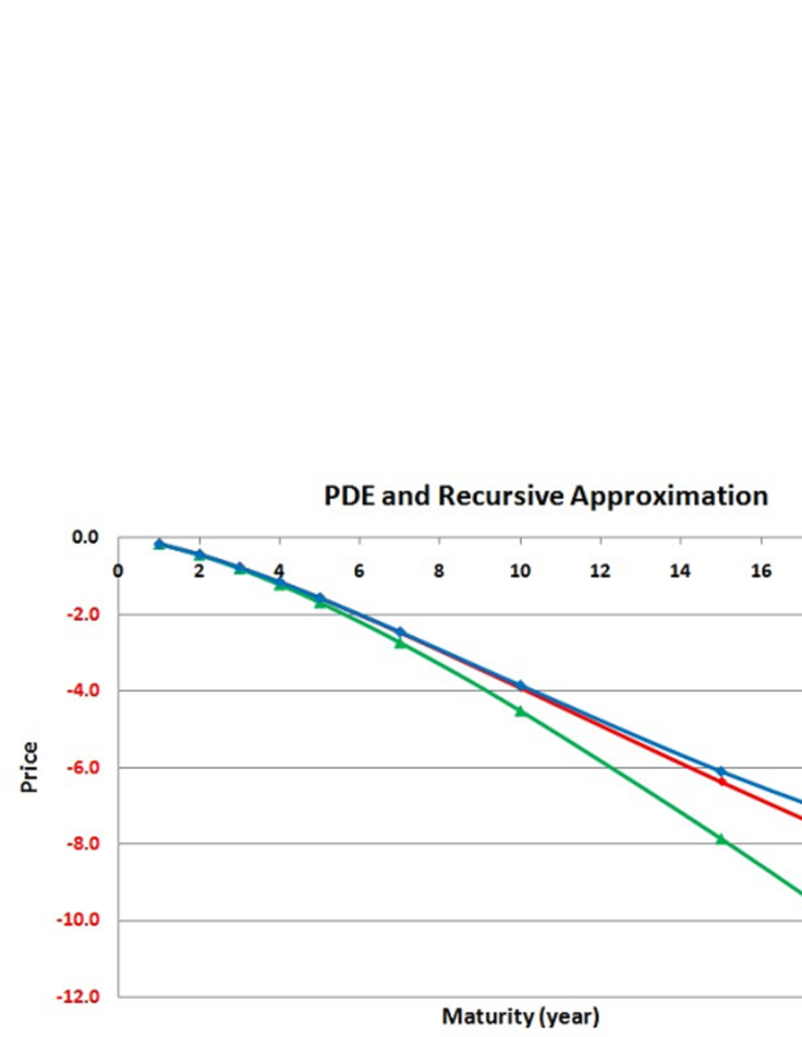
Figure 1: Numerical Comparison to PDE

In Fig. 1, we have plot the numerical results of the forward contract with bilateral default risk with various maturities with the direct solution from the PDE. We have used

$$r=0.02,\quad\lambda=0.01,\quad h=0.03,$$ (3.28)

$$\sigma=0.2,\quad S_{0}=100~{},$$ (3.29)

where the strike $K$ is chosen to make $V^{(0)}_{0}=0$ for each maturity. We have plot $V^{(1)}$ for the first order, and $V^{(1)}+V^{(2)}$ for the second order. Note that we have put $\epsilon=1$ to compare the original model. One can observe how the higher order correction improves the accuracy of approximation. In this example, the counterparty is significantly riskier than the investor, and the underlying contract is quite volatile . Even in this situation, the simple approximation to the second order works quite well up to the very long maturity.

3.2 A self-financing portfolio with differential interest rates

In this subsection, we consider the valuation of self-financing portfolio under the situation where there exists a difference between the lending and borrowing interest rates. Here, we consider the problem under the physical measure.

The dynamics of the self-financing portfolio is governed by [4]

$$dV_{t} = rV_{t}dt-\left\{(R-r)\max\left(\frac{Z_{t}}{\sigma}-V_{t},0\right)-\theta Z_{t}\right\}dt+Z_{t}dW_{t}$$ (3.30)

$$V_{T} = \Phi(S_{T})$$ (3.31)

$$dS_{t} = S_{t}\Bigl{(}\mu dt+\sigma dW_{t}\Bigr{)}$$ (3.32)

where $r$ and $R$ are the lending and the borrowing rate, respectively. $\theta=(\mu-r)/\sigma$ denotes the risk premium. For simplicity, we assume all of the $r$, $R$, $\mu$ and $\sigma$ are positive constants. Here, $Z_{t}/\sigma$ represents the amount invested in the risky asset, i.e. stock $S_{t}$. Let us choose the terminal wealth function as

$$\Phi(S_{T})=\max(S_{T}-K_{1},0)-2\max(S_{T}-K_{2},0)~{}.$$ (3.33)

This spread introduces both of the lending and borrowing activities, which makes the problem more interesting. The setup explained here is in fact exactly the same as that of adopted by Gobet et al. (2005) [6]. They have carried our detailed numerical studies for the above problem and evaluate $V_{0}$ by regression-based Monte Carlo simulation. In the following, we will apply our perturbative approximation scheme to the same problem and test its accuracy.

As usual, let us introduce the expansion parameter as

$$dV_{t}^{(\epsilon)} = rV_{t}^{(\epsilon)}dt-\epsilon g(V_{t}^{(\epsilon)},Z_{t}^{(\epsilon)})dt+Z_{t}^{(\epsilon)}dW_{t}$$ (3.34)

$$V_{T}^{(\epsilon)} = \Phi(S_{T})~{},$$ (3.35)

where we have defined the non-linear perturbation function as

$$g(v,z)=(R-r)\max\left(\frac{z}{\sigma}-v,0\right)-\theta z~{}.$$ (3.36)

Now, we are going to expand $V_{t}^{(\epsilon)}$ in terms of $\epsilon$.

3.2.1 Zero-th order

In the zero-th order, the BSDE reduces to

$$dV_{t}^{(0)} = rV_{t}^{(0)}dt+Z_{t}^{(0)}dW_{t}$$ (3.37)

$$V_{T}^{(0)} = \Phi(S_{T})~{},$$ (3.38)

which allows us to obtain

$$V_{t}^{(0)} = E\left[\left.e^{-r(T-t)}\Bigl{\{}(S_{T}-K_{1})^{+}-2(S_{T}-K_{2})^{+}\Bigr{\}}\right|{\cal F}_{t}\right]$$ (3.39)

$$= e^{-r(T-t)}\left(C(K_{1},S_{t})-2C(K_{2},S_{t})\right)~{},$$ (3.40)

where we have defined

$$C(K_{i},S_{t}) = S_{t}e^{\mu(T-t)}N\bigl{(}d_{1}(K_{i},S_{t})\bigr{)}-K_{i}N\bigl{(}d_{2}(K_{i},S_{t})\bigr{)}$$ (3.41)

$$d_{1(2)}(K_{i},S_{t}) = \frac{1}{\sigma\sqrt{T-t}}\left\{\ln\left(\frac{S_{t}e^{\mu(T-t)}}{K_{i}}\right)\pm\frac{1}{2}\sigma^{2}(T-t)\right\}~{}$$ (3.42)

for $i\in\{1,2\}$. The volatility term is given by

$$Z_{t}^{(0)}=e^{(\mu-r)(T-t)}\sigma S_{t}\Bigl{(}N\bigl{(}d_{1}(K_{1},S_{t})\bigr{)}-2N\bigl{(}d_{2}(K_{2},S_{t})\bigr{)}\Bigr{)}~{}.$$ (3.43)

3.2.2 First order

Now, in the first order, we have

$$dV_{t}^{(1)} = rV_{t}^{(1)}dt-g(V_{t}^{(0)},Z_{t}^{(0)})dt+Z_{t}^{(1)}dW_{t}$$ (3.44)

$$V_{T}^{(1)} = 0~{}.$$ (3.45)

As before, we can easily integrate it to obtain

$$V_{t}^{(1)}=E\left[\left.\int_{t}^{T}e^{-r(u-t)}g(V_{u}^{(0)},Z_{u}^{(0)})du\right|{\cal F}_{t}\right]~{}.$$ (3.46)

Now, using the zero-th order results, one can show

$$g(V_{t}^{(0)},Z_{t}^{(0)}) = e^{-r(T-t)}(R-r)\Bigl{\{}K_{1}N(d_{2}(K_{1},S_{t}))-2K_{2}N(d_{2}(K_{2},S_{t}))\Bigr{\}}^{+}$$ (3.47)

$$- e^{-r(T-t)}(\mu-r)S_{t}e^{\mu(T-t)}\Bigl{\{}N(d_{1}(K_{1},S_{t}))-2N(d_{1}(K_{2},S_{t}))\Bigr{\}}~{},$$

which leads to

$$V_{t}^{(1)} = e^{-r(T-t)}\int_{t}^{T}du\left\{E\left[(R-r)\Bigl{(}K_{1}N(d_{2}(K_{1},S_{u}))-2K_{2}N(d_{2}(K_{2},S_{u}))\Bigr{)}^{+}\right.\right.$$

$$\hskip 56.9055pt-\left.\left.\left.(\mu-r)S_{u}e^{\mu(T-u)}\Bigl{(}N(d_{1}(K_{1},S_{u}))-2N(d_{1}(K_{2},S_{u}))\Bigr{)}\right|{\cal F}_{t}\right]\right\}~{}.$$

By setting

$$S_{u}(S_{t},z)=S_{t}e^{\mu(u-t)}\exp\left(-\frac{1}{2}\sigma^{2}(u-t)+\sigma\sqrt{u-t}z\right)$$ (3.49)

we can write the first order correction as

$$V_{t}^{(1)}=e^{-r(T-t)}\int_{t}^{T}du\int_{\mathbb{R}}dz\phi(z)$$

$$\hskip 28.45274pt\left\{(R-r)\Bigl{[}K_{1}N(d_{2}(K_{1},S_{u}(S_{t},z)))-2K_{2}N(d_{2}(K_{2},S_{u}(S_{t},z)))\Bigr{]}^{+}\right.$$

$$\hskip 28.45274pt-\left.(\mu-r)S_{u}(S_{t},z)e^{\mu(T-u)}\Bigl{[}N(d_{1}(K_{1},S_{u}(S_{t},z)))-2N(d_{1}(K_{2},S_{u}(S_{t},z)))\Bigr{]}\right\}~{}.$$

The volatility term can also be derived easily as

$$Z_{t}^{(1)} = \sigma S_{t}\frac{\partial}{\partial S_{t}}V_{t}^{(1)}(S_{t})$$ (3.51)

$$= e^{-r(T-t)}\int_{t}^{T}du\int_{\mathbb{R}}dz\phi(z)\Bigl{[}$$

$$\chi(u,z)\frac{1}{\sqrt{T-u}}\Bigl{(}K_{1}\phi(d_{2}(K_{1};S_{u}(S_{t},z)))-2K_{2}\phi(d_{2}(K_{2},S_{u}(S_{t},z)))\Bigr{)}$$

$$-(\mu-r)S_{u}(S_{t},z)e^{\mu(T-u)}\Bigl{\{}\sigma\Bigl{(}N(d_{1}(K_{1},S_{u}(S_{t},z)))-2N(d_{1}(K_{2},S_{u}(S_{t},z)))\Bigr{)}$$

$$\quad+\frac{1}{\sqrt{T-u}}\Bigl{(}\phi(d_{1}(K_{1},S_{u}(S_{t},z)))-2\phi(d_{1}(K_{2},S_{u}(S_{t},z)))\Bigr{)}\Bigr{\}}\Bigr{]}~{},$$

where we have defined

$$\chi(u,z) = 1~{}\quad{\mbox{if}}~{}\quad K_{1}N(d_{2}(K_{1},S_{u}(S_{t},z)))-2K_{2}N(d_{2}(K_{2},S_{u}(S_{t},z)))\geq 0$$ (3.52)

$$= 0~{}\quad{\mbox{otherwise}}~{}.$$

3.2.3 Second order

Finally, in the second order, the relevant FBSDE is given by

$$dV_{t}^{(2)} = rV_{t}^{(2)}dt-\left(\frac{\partial}{\partial v}g(V_{t}^{(0)},Z_{t}^{(0)})V_{t}^{(1)}+\frac{\partial}{\partial z}g(V_{t}^{(0)},Z_{t}^{(0)})Z_{t}^{(1)}\right)dt+Z_{t}^{(2)}dW_{t}$$

$$V_{T}^{(2)} = 0~{}.$$ (3.53)

Using the fact that

$$\frac{\partial}{\partial v}g(v,z) = -(R-r)\mathbb{1}_{\{\frac{z}{\sigma}-v\geq 0\}}$$ (3.54)

$$\frac{\partial}{\partial z}g(v,z) = \frac{R-r}{\sigma}\mathbb{1}_{\{\frac{z}{\sigma}-v\geq 0\}}-\theta$$ (3.55)

we obtain

$$V_{t}^{(2)}=e^{-r(T-t)}\int_{t}^{T}du\int_{u}^{T}ds\int_{\mathbb{R}}dz_{1}\int_{\mathbb{R}}dz_{2}\phi(z_{1})\phi(z_{2})\Bigl{[}$$

$$\quad\chi(u,z_{1})\Bigl{\{}-(R-r)^{2}\Bigl{(}K_{1}N\bigl{(}d_{2}(K_{1},S_{s}(u,\vec{z}))\bigr{)}-2K_{2}N\bigl{(}d_{2}(K_{2},S_{s}(u,\vec{z}))\bigr{)}\Bigr{)}^{+}$$

$$+(R-r)(\mu-r)S_{s}(u,\vec{z})e^{\mu(T-s)}\Bigl{(}N(d_{1}(K_{1};S_{s}(u,\vec{z})))-2N(d_{1}(K_{2},S_{s}(u,\vec{z})))\Bigr{)}\Bigr{\}}$$

$$+\left(\frac{R-r}{\sigma}\chi(u,z_{1})-\theta\right)\Bigl{\{}$$

$$(R-r)\chi(s,u,\vec{z})\frac{1}{\sqrt{T-s}}\Bigl{(}K_{1}\phi(d_{2}(K_{1},S_{s}(u,\vec{z})))-2K_{2}\phi(d_{2}(K_{2},S_{s}(u,\vec{z})))\Bigr{)}$$

$$-(\mu-r)S_{s}(u,\vec{z})e^{\mu(T-s)}\Bigl{(}\sigma[N(d_{1}(K_{1},S_{s}(u,\vec{z})))-2N(d_{2}(K_{2},S_{s}(u,\vec{z})))]$$

$$\hskip 56.9055pt\left.\left.+\frac{1}{\sqrt{T-s}}[\phi(d_{1}(K_{1},S_{s}(u,\vec{z})))-2\phi(d_{1}(K_{2},S_{s}(u,\vec{z})))]\right)\Bigr{\}}\right]~{}.$$ (3.56)

Here, we have defined

$$S_{s}(u,\vec{z}) = S_{s}(S_{u}(S_{t},z_{1}),z_{2})$$ (3.57)

and also

$$\chi(s,u,\vec{z}) = 1\quad\mbox{if}\quad K_{1}N(d_{2}(K_{1},S_{s}(u,\vec{z})))-2K_{2}N(d_{2}(K_{2},S_{s}(u,\vec{z})))\geq 0$$ (3.58)

$$= 0\quad\mbox{otherwise}~{}.$$

If one needs, it is also straightforward to derive the volatility component.

3.2.4 Numerical comparison to the result of Gobet et al.

Gobet et al. (2005) [6] have carried out the detailed numerical study for the above problem using the regression-based Monte Carlo simulation. They have used

$$\mu=0.05,\quad\sigma=0.2,\quad r=0.01,\quad R=0.06$$

$$T=0.25,\quad S_{0}=100,\quad K_{1}=95,\quad K_{2}=105~{}.$$ (3.59)

After trying various sets of basis functions, they have obtained the price as $V_{0}=2.95$ with standard deviation $0.01$.

Now, let us provide the results from our perturbative expansion. We have obtained

$$V_{0}^{(0)}=2.7863$$

$$V_{0}^{(1)}=0.1814$$

$$V_{0}^{(2)}=-0.0149$$

using the same model inputs. Thus, up to the first order, we have $V_{0}^{(0)}+V_{0}^{(1)}=2.968$, which is already fairly close, and once we include the second order correction, we have $\sum_{i=0}^{2}V_{0}^{(i)}=2.953$, which is perfectly consistent with their result of Monte Carlo simulation. Note that, we have derived analytic formulas with explicit expressions both for the contract value and its volatility.

4 Application of Asymptotic Expansion to Generic Markovian Forward Processes

In this section, we consider the situation where the forward components $\{X_{t}\}$ consist of the generic Markovian processes. In this case, we cannot express $V_{t}^{(i)}$ and $Z_{t}^{(i)}$ in terms of $\{X_{t}\}$ exactly, which prohibits us from obtaining the higher order corrections in a simple fashion as we have done in the previous section.

However, notice the fact that what we have to do in each order of expansion is equivalent to the pricing of generic European contingent claims and hence we can borrow known techniques adopted there. In the following, we will explain the use of asymptotic expansion method, now for the forward components. Although it is impossible to obtain the exact result, we can still obtain analytic expression for $(V_{t}^{(i)},Z_{t}^{(i)})$ up to a certain order of the volatilities of $\{X_{t}\}$. For the details of asymptotic expansion for volatility, please consult with the works [7, 11, 12, 13, 14], for example.

Let us introduce a new expansion parameter $\delta$, which is now for the asymptotic expansion for the forward components. We express the relevant SDE of generic Markovian process $X^{(\delta)}\in\mathbb{R}^{d}$ as

$$dX_{u}^{(\delta)}=\gamma_{0}(X_{u}^{(\delta)},\delta)du+\gamma_{a}(X_{u}^{(\delta)},\delta)dW_{u}^{a}~{}.$$ (4.1)

Here, we have used Einstein notation which assumes the summation of all the paired indexes. For example, in the above equation, the second term means

$$\gamma_{a}(X_{u}^{(\delta)},\delta)dW_{u}^{a}=\sum_{a=1}^{r}\gamma_{a}(X_{u}^{(\delta)},\delta)dW_{u}^{a}~{}.$$ (4.2)

We assume

$$\gamma_{a}(x,0)=0$$ (4.3)

for $a=\{1,\cdots,r\}$. Intuitively speaking, it suggests that $\delta$ counts the order of volatility.

Suppose that, in the $(i-1)$-th order of $\epsilon$, we succeeded to express $V_{t}^{(i-1)}$ and $Z_{t}^{(i-1)}$ in terms of $X_{t}^{(\delta)}$. Then, in the next order, we can express the backward components as

$$V_{t}^{(i)} = E\left[\left.\int_{t}^{T}e^{-\int_{t}^{u}c(X_{s}^{(\delta)})ds}G(X_{u}^{(\delta)},\delta)du\right|{\cal F}_{t}\right]$$ (4.4)

$$Z_{t}^{(i)} = E\left[\left.{\cal D}_{t}\left(\int_{t}^{T}e^{-\int_{t}^{u}c(X_{s}^{(\delta)})ds}G(X_{u}^{(\delta)},\delta)du\right)\right|{\cal F}_{t}\right]$$ (4.5)

with some function $G$. If there is no need to obtain $(V_{t}^{(i+1)},Z_{t}^{(i+1)})$, we can just run Monte Carlo simulation for $X^{(\delta)}$ to evaluate these quantities in a standard way. However, if we want to obtain higher order corrections, we need somehow to express the $(V_{t}^{(i)},Z_{t}^{(i)})$ in terms of $X_{t}^{(\delta)}$.

What we are going to propose here is to expand the backward components around $\delta=0$:

$$V_{t}^{(i)} = V_{t}^{(i,0)}+\delta V_{t}^{(i,1)}+\delta^{2}V_{t}^{(i,2)}+o(\delta^{2})$$ (4.6)

$$Z_{t}^{(i)} = Z_{t}^{(i,0)}+\delta Z_{t}^{(i,1)}+\delta^{2}Z_{t}^{(i,2)}+o(\delta^{2})$$ (4.7)

and express each $V_{t}^{(i,j)}$ and $Z_{t}^{(i,j)}$ in terms of $X_{t}^{(\delta)}$ up to a certain order ”$j$” of $\delta$. Although we can proceed to arbitrarily higher order of $\delta$, we will present explicit expressions up to the second order in this paper. For the interested readers, the work [13] provides the systematic methods to obtain higher order corrections.

Thank to the well-known chain rule for Malliavin derivative, what we have to do is only expanding the two fundamental quantities, $X_{u}$ and ${\cal D}_{t}X_{u}$ for $u\in[t,T]$, in terms of $\delta$. Firstly, let us introduce a simpler notation,

$$dX_{u}^{(\delta)} = \gamma_{0}(X_{u}^{(\delta)},\delta)du+\gamma_{a}(X_{u}^{(\delta)},\delta)dW_{u}^{a}$$ (4.8)

$$:= \gamma_{\alpha}(X_{u}^{(\delta)},\delta)dw_{u}^{\alpha}~{},$$

where $\alpha$ runs through $0$ to $r$ with the convention $w_{u}^{0}=u$ and $w_{u}^{a}=W_{u}^{a}$ for $a\in\{1,\cdots,r\}$. We set the time $t$-value of $X^{(\delta)}$ as $x$. Thus our goal is to express $V^{(i,j)}$ and $Z^{(i,j)}$ as functions of $x$. We first introduce a $d\times d$ matrix process $Y^{(\delta)}$ defined as

$$d(Y_{t,u}^{(\delta)})^{i}_{j} = \partial_{k}\gamma^{i}_{\alpha}(X_{u}^{(\delta)},\delta)(Y_{t,u}^{(\delta)})^{k}_{j}dw_{u}^{\alpha}$$ (4.9)

$$(Y_{t,t}^{(\delta)})^{i}_{j} = \delta^{i}_{j}~{},$$ (4.10)

where $\partial_{k}$ denotes the differential with respect to the $k$-th component of $X$. Since we have

$$(X_{u}^{(\delta)})^{i}=x^{i}+\int_{t}^{u}\gamma^{i}_{0}(X_{s}^{(\delta)},\delta)ds+\int_{t}^{u}\gamma^{i}_{a}(X_{s}^{(\delta)},\delta)dW_{s}^{a}$$ (4.11)

applying a Malliavin derivative ${\cal D}_{t,\beta}$ with $\beta\in\{1,\cdots,r\}$ gives

$${\cal D}_{t,\beta}(X_{u}^{(\delta)})^{i}=\int_{t}^{u}\partial_{k}\gamma_{0}^{i}(X_{s}^{(\delta)},\delta){\cal D}_{t,\beta}(X_{s}^{(\delta)})^{k}ds+\int_{t}^{u}\partial_{k}\gamma^{i}_{a}(X_{s}^{(\delta)},\delta){\cal D}_{t,\beta}(X_{s}^{(\delta)})^{k}dW_{s}^{a}+\gamma^{i}_{\beta}(x,\delta)~{}.$$

Thus one can show that

$$d\bigl{(}{\cal D}_{t,\beta}(X_{u}^{(\delta)})^{i}\bigr{)} = \partial_{k}\gamma^{i}_{\alpha}(X_{u}^{(\delta)},\delta){\cal D}_{t,\beta}(X_{u}^{(\delta)})^{k}dw_{u}^{\alpha}$$ (4.12)

$${\cal D}_{t,\beta}(X_{t}^{(\delta)})^{i} = \gamma^{i}_{\beta}(x,\delta)~{}.$$ (4.13)

Therefore, for $a\in\{1,\cdots,r\}$, we conclude that

$${\cal D}_{t,a}(X_{u}^{(\delta)})^{i}=(Y^{(\delta)}_{t,u})^{i}_{j}\gamma^{j}_{a}(x,\delta)~{},$$ (4.14)

which implies that the asymptotic expansion of ${\cal D}_{t}X_{u}^{(\delta)}$ can be obtained from that of $Y^{(\delta)}$. Therefore, in the following, we first carry out the asymptotic expansion for $X$ and $Y$.

4.1 Asymptotic Expansion for $X_{u}^{(\delta)}$ and $Y_{u}^{(\delta)}$

We are now going to expand for $u\in[t,T]$ as

$$X_{u}^{(\delta)}=X_{u}^{(0)}+\delta D_{t,u}+\frac{1}{2}\delta^{2}E_{t,u}+o(\delta^{2})~{},$$ (4.15)

and

$$Y_{t,u}^{(\delta)}=Y_{t,u}+\delta H_{t,u}+o(\delta)~{},$$ (4.16)

where

$$D_{t,u}=\left.\frac{\partial X_{u}^{(\delta)}}{\partial\delta}\right|_{\delta=0},\qquad E_{t,u}=\left.\frac{\partial^{2}X_{u}^{(\delta)}}{\partial\delta^{2}}\right|_{\delta=0}~{},$$ (4.17)

and

$$Y_{t,u}=Y_{t,u}^{(0)},\qquad H_{t,u}=\left.\frac{\partial Y_{t,u}^{(\delta)}}{\partial\delta}\right|_{\delta=0}~{}.$$ (4.18)

4.1.1 Zero-th order

Since $\gamma_{a}(\cdot,0)=0$ for $a\in\{1,\cdots,r\}$, we have

$$dX_{u}^{(0)} = \gamma_{0}(X_{u}^{(0)},0)du$$ (4.19)

$$d(Y_{t,u})^{i}_{j} = \partial_{k}\gamma^{i}_{0}(X_{u}^{(0)},0)(Y_{t,u})^{k}_{j}du$$ (4.20)

with the initial conditions $X_{t}^{(0)}=x$ and $(Y_{t,t})^{i}_{j}=\delta^{i}_{j}$, which allows us to express $X_{u}^{(0)}$ and $Y_{t,u}$ as deterministic functions of $x$. It is also convenient for later calculations to notice that $Y^{-1}$ is the solution of

$$d(Y^{-1}_{t,u})^{i}_{j} = -(Y_{t,u}^{-1})^{i}_{k}\partial_{j}\gamma_{0}^{k}(X_{u}^{(0)},0)du$$ (4.21)

with $(Y^{-1}_{t,t})^{i}_{j}=\delta^{i}_{j}$.

4.1.2 First order

By applying $\partial_{\delta}$, we can easily obtain

$$d(\partial_{\delta}X_{u}^{(\delta)})^{i} = (\partial\gamma_{\alpha}(X_{u}^{(\delta)},\delta))^{i}_{j}\partial_{\delta}(X_{u}^{(\delta)})^{j}dw_{u}^{\alpha}+\partial_{\delta}\gamma^{i}_{\alpha}(X_{u}^{(\delta)},\delta)dw_{u}^{\alpha}$$ (4.22)

$$d(\partial_{\delta}Y^{(\delta)}_{t,u})^{i}_{j} = \Bigl{\{}\partial_{k}\gamma^{i}_{\alpha}(X_{u}^{(\delta)},\delta)(\partial_{\delta}Y^{(\delta)}_{t,u})^{k}_{j}+\partial_{kl}\gamma^{i}_{\alpha}(X_{u}^{(\delta)},\delta)(\partial_{\delta}X_{u}^{(\delta)})^{l}(Y_{t,u}^{(\delta)})^{k}_{j}$$

$$+\partial_{k}\partial_{\delta}\gamma^{i}_{\alpha}(X_{u}^{(\delta)},\delta)(Y_{t,u}^{(\delta)})^{k}_{j}\Bigr{\}}dw_{u}^{\alpha}~{}.$$

Putting $\delta=0$, they leads to

$$dD^{i}_{t,u} = \partial_{j}\gamma^{i}_{0}(X_{u}^{(0)},0)D^{j}_{t,u}du+\partial_{\delta}\gamma^{i}_{\alpha}(X_{u}^{(0)},0)dw_{u}^{\alpha}$$ (4.24)

$$d(H_{t,u})^{i}_{j} = (\partial_{k}\gamma^{i}_{0}(X_{u}^{(0)},0))(H_{t,u})^{k}_{j}du+\partial_{kl}\gamma^{i}_{0}(X_{u}^{(0)},0))D^{l}_{t,u}(Y_{t,u})^{k}_{j}du$$ (4.25)

$$+(\partial_{k}\partial_{\delta}\gamma^{i}_{\alpha}(X_{u}^{(0)},0))(Y_{t,u})^{k}_{j}dw_{u}^{\alpha}~{}.$$

Now, by using Eq.(4.21), one can show that

$$D^{i}_{t,u}=(Y_{t,u})^{i}_{j}\int_{t}^{u}(Y_{t,s}^{-1})^{j}_{k}\partial_{\delta}\gamma_{\alpha}^{k}(s)dw_{s}^{\alpha}$$ (4.26)

$$(H_{t,u})^{i}_{j}=(Y_{t,u})^{i}_{k}\int_{t}^{u}(Y^{-1}_{t,s})^{k}_{l}\Bigl{\{}(\partial_{mn}\gamma^{l}_{0}(s))D^{n}_{t,s}(Y_{t,s})^{m}_{j}ds+(\partial_{m}\partial_{\delta}\gamma^{l}_{\alpha}(s))(Y_{t,s})^{m}_{j}dw_{s}^{\alpha}\Bigr{\}}$$

where we have defined the shorthand notation that

$$\gamma^{i}_{j}(s):=\gamma^{i}_{j}(X_{s}^{(0)},0),$$ (4.28)

which will be used in the following calculations, too.

4.1.3 Second order

Applying $\partial_{\delta}^{2}$ to the SDE of $X^{(\delta)}$ gives us

$$d(\partial_{\delta}^{2}X_{u}^{(\delta)})^{i} = \Bigl{\{}(\partial\gamma_{\alpha}(X_{u}^{(\delta)},\delta))^{i}_{j}\partial_{\delta}^{2}(X_{u}^{(\delta)})^{j}+\partial_{jk}\gamma^{i}_{\alpha}(X_{u}^{(\delta)},\delta)\partial_{\delta}(X_{u}^{(\delta)})^{j}\partial_{\delta}(X_{u}^{(\delta)})^{k}$$ (4.29)

$$+2\partial_{j}\partial_{\delta}\gamma^{i}_{\alpha}(X_{u}^{(\delta)},\delta)\partial_{\delta}(X_{u}^{(\delta)})^{j}+\partial_{\delta}^{2}\gamma^{i}_{\alpha}(X_{u}^{(\delta)},\delta)\Bigr{\}}dw_{u}^{\alpha}~{}.$$

Thus, putting $\delta=0$, we obtain

$$dE^{i}_{t,u} = (\partial\gamma_{0}(X_{u}^{(0)},0))^{i}_{j}E^{j}_{t,u}du+\partial_{jk}\gamma^{i}_{0}(X_{u}^{(0)},0)D^{j}_{t,u}D^{k}_{t,u}du$$ (4.30)

$$+2\partial_{j}\partial_{\delta}\gamma^{i}_{\alpha}(X_{u}^{(0)},0)D^{j}_{t,u}dw_{u}^{\alpha}+\partial_{\delta}^{2}\gamma^{i}_{\alpha}(X_{u}^{(0)},0)dw_{u}^{\alpha}~{}.$$

Now we can integrate it as

$$E^{i}_{t,u}=(Y_{t,u})^{i}_{j}\int_{t}^{u}(Y^{-1}_{t,s})^{j}_{k}\Bigl{\{}\partial_{lm}\gamma^{k}_{0}(s)D^{l}_{t,s}D^{m}_{t,s}ds+\Bigl{(}2\partial_{l}\partial_{\delta}\gamma^{k}_{\alpha}(s)D^{l}_{t,s}+\partial_{\delta}^{2}\gamma^{k}_{\alpha}(s)\Bigr{)}dw_{s}^{\alpha}\Bigr{\}}.~{}$$

We do not need the second order terms for $Y^{(\delta)}$.

4.2 Asymptotic Expansion for Malliavin Derivative: ${\cal D}_{t}X_{u}^{(\delta)}$

For convenience, let us define

$$({\cal X}_{a}^{i})^{(\delta)}_{t,u}=({\cal D}_{t}X_{u}^{(\delta)})^{i}_{a}$$ (4.32)

and its expansion as

$$({\cal X}_{a}^{i})^{(\delta)}_{t,u}=\delta({\cal X}_{a}^{i})^{(1)}_{t,u}+\frac{1}{2}\delta^{2}({\cal X}_{a}^{i})^{(2)}_{t,u}+o(\delta^{2})~{},$$ (4.33)

where

$$({\cal X}_{a}^{i})_{t,u}^{(1)}=\left.\frac{\partial}{\partial\delta}({\cal X}_{a}^{i})^{(\delta)}_{t,u}\right|_{\delta=0},\qquad({\cal X}_{a}^{i})_{t,u}^{(2)}=\left.\frac{\partial^{2}}{\partial\delta^{2}}({\cal X}_{a}^{i})^{(\delta)}_{t,u}\right|_{\delta=0}~{}.$$ (4.34)

Note that, the zero-th order term $({\cal X}_{a}^{i})^{(0)}$ vanishes, due to the assumption (4.3).

From (4.14), we can easily show that

$$({\cal X}_{a}^{i})^{(1)}_{t,u} = (Y_{t,u})^{i}_{j}(\partial_{\delta}\gamma^{j}_{a}(x,0))$$ (4.35)

$$({\cal X}_{a}^{i})^{(2)}_{t,u} = (Y_{t,u})^{i}_{j}(\partial_{\delta}^{2}\gamma^{j}_{a}(x,0))+2(H_{t,u})^{i}_{j}(\partial_{\delta}\gamma^{j}_{a}(x,0))~{}.$$ (4.36)

4.3 Asymptotic Expansion for $V^{(i,\delta)}$

Now, we try to express

$$V_{t}^{(i,\delta)}=\int_{t}^{T}E\left[\left.e^{-\int_{t}^{u}c(X_{s}^{(\delta)})ds}G(X_{u}^{(\delta)},\delta)\right|{\cal F}_{t}\right]du$$ (4.37)

as a function of $x=X_{t}^{(\delta)}$ using the previous results. For that purpose, we first need to carry out asymptotic expansion for

$$R_{t,u}^{(\delta)}:=e^{-\int_{t}^{u}c(X_{s}^{(\delta)})ds}G(X_{u}^{(\delta)},\delta)~{}$$ (4.38)

to obtain

$$R^{(\delta)}_{t,u}=R^{(0)}_{t,u}+\delta R^{(1)}_{t,u}+\frac{1}{2}\delta^{2}R^{(2)}_{t,u}+o(\delta^{2})~{},$$ (4.39)

where

$$R^{(1)}_{t,u}=\left.\frac{\partial}{\partial\delta}R^{(\delta)}_{t,u}\right|_{\delta=0}~{},\qquad R^{(2)}_{t,u}=\left.\frac{\partial^{2}}{\partial\delta^{2}}R^{(\delta)}_{t,u}\right|_{\delta=0}~{}.$$ (4.40)

Then, we can take the conditional expectation straightforwardly.

4.3.1 Zero-th order

We have

$$R^{(0)}_{t,u}=e^{-\int_{t}^{u}c(X_{s}^{(0)})ds}G(X_{u}^{(0)},0)$$ (4.41)

which is a deterministic function of $x$.

4.3.2 First order

It is easy to obtain

$$\partial_{\delta}R^{(\delta)}_{t,u} = e^{-\int_{t}^{u}c(X_{s}^{(\delta)})ds}\Bigl{\{}-G(X_{u}^{(\delta)},\delta)\int_{t}^{u}\partial_{i}c(X_{s}^{(\delta)})(\partial_{\delta}X_{s}^{(\delta)})^{i}ds$$ (4.42)

$$\qquad+(\partial_{i}G(X_{u}^{(\delta)},\delta))(\partial_{\delta}X_{u}^{(\delta)})^{i}+\partial_{\delta}G(X_{u}^{(\delta)},\delta)\Bigr{\}}~{},$$

which leads to

$$R^{(1)}_{t,u}=e^{-\int_{t}^{u}c(X_{s}^{(0)})ds}\Bigl{\{}(\partial_{i}G(X_{u}^{(0)},0))D_{t,u}^{i}+\partial_{\delta}G(X_{u}^{(0)},0)-G(X_{u}^{(0)},0)\int_{t}^{u}\partial_{i}c(X_{s}^{(0)})D^{i}_{t,s}ds\Bigr{\}}.$$

4.3.3 Second order

In the same way, we can show that

$$R^{(2)}_{t,u} = e^{-\int_{t}^{u}c(X_{s}^{(0)})ds}\Bigl{\{}(\partial_{ij}G(X_{u}^{(0)},0))D^{i}_{t,u}D^{j}_{t,u}+2(\partial_{i}\partial_{\delta}G(X_{u}^{(0)},0))D^{i}_{t,u}$$ (4.44)

$$\qquad+(\partial_{i}G(X_{u}^{(0)},0))E^{i}_{t,u}+\partial_{\delta}^{2}G(X_{u}^{(0)},0)$$

$$\qquad+\left(\int_{t}^{u}\partial_{i}c(X_{s}^{(0)})D^{i}_{t,s}ds\right)^{2}G(X_{u}^{(0)},0)$$

$$\qquad-2\left(\int_{t}^{u}\partial_{i}c(X_{s}^{(0)})D^{i}_{t,s}ds\right)\Bigl{(}\partial_{j}G(X_{u}^{(0)},0)D^{j}_{t,u}+\partial_{\delta}G(X_{u}^{(0)},0)\Bigr{)}$$

$$\qquad-\left(\int_{t}^{u}\bigl{[}\partial_{ij}c(X_{s}^{(0)})D^{i}_{t,s}D^{j}_{t,s}+\partial_{i}c(X_{s}^{(0)})E^{i}_{t,s}\Bigr{]}ds\right)G(X_{u}^{(0)},0)\Bigr{\}}~{}.$$

4.3.4 Expression for $V_{t}^{(i,\delta)}$

Evaluation of the conditional expectation can be easily done by simply applying Ito-isometry. Let us first define

$$\overline{D}^{i}_{t,u} = (Y_{t,u})^{i}_{j}\int_{t}^{u}(Y_{t,s}^{-1})^{j}_{k}(\partial_{\delta}\gamma^{k}_{0}(s))ds$$ (4.45)

$$\hat{D}^{i}_{t,u} = (Y_{t,u})^{i}_{j}\int_{t}^{u}(Y_{t,s}^{-1})^{j}_{k}(\partial_{\delta}\gamma^{k}_{a}(s))dW^{a}_{s}$$ (4.46)

and then we have $D^{i}_{t,u}=\overline{D}^{i}_{t,u}+\hat{D}^{i}_{t,u}$. Since the first one is a deterministic function, we have, for $\forall u,s\geq t$,

$$\overline{D^{i}_{t,u}D^{j}_{t,s}} := E\left[\left.D^{i}_{t,u}D^{j}_{t,s}\right|{\cal F}_{t}\right]$$ (4.47)

$$= \overline{D}^{i}_{t,u}\overline{D}^{j}_{t,s}+\overline{\hat{D}^{i}_{t,u}\hat{D}^{j}_{t,s}}~{},$$

where

$$\overline{\hat{D}^{i}_{t,u}\hat{D}^{j}_{t,s}}=(Y_{t,u})^{i}_{k}(Y_{t,s})^{j}_{l}\int_{t}^{u\wedge s}(Y^{-1}_{t,v})^{k}_{m}(Y^{-1}_{t,v})^{l}_{n}(\partial_{\delta}\gamma^{m}_{a}(v))(\partial_{\delta}\gamma^{n}_{a}(v))dv~{}.$$ (4.48)

Then, similarly, we can express

$$\overline{E}_{t,u}^{i}:=E\left[\left.E_{t,u}^{i}\right|{\cal F}_{t}\right]$$

$$\quad=(Y_{t,u})^{i}_{j}\int_{t}^{u}(Y_{t,s}^{-1})^{j}_{k}\Bigl{\{}\partial_{lm}\gamma^{k}_{0}(s)\overline{D^{l}_{t,s}D^{m}_{t,s}}+2\partial_{l}\partial_{\delta}\gamma^{k}_{0}(s)\overline{D}^{l}_{t,s}+\partial_{\delta}^{2}\gamma^{k}_{0}(s)\Bigr{\}}ds~{}.$$ (4.49)

Using these results, we have

$$\overline{R}^{(0)}_{t,u}:=E\left[\left.R_{t,u}^{(0)}\right|{\cal F}_{t}\right]=e^{-\int_{t}^{u}c(X_{s}^{(0)})ds}G(X_{u}^{(0)},0)$$ (4.50)

$$\overline{R}^{(1)}_{t,u}:=E\left[\left.R_{t,u}^{(1)}\right|{\cal F}_{t}\right]$$

$$~{}~{}=e^{-\int_{t}^{u}c(X_{s}^{(0)})ds}\Bigl{\{}(\partial_{i}G(X_{u}^{(0)},0))\overline{D}^{i}_{t,u}+\partial_{\delta}G(X_{u}^{(0)},0)-G(X_{u}^{(0)},0)\int_{t}^{u}\partial_{i}c(X_{s}^{(0)})\overline{D}^{i}_{t,s}ds\Bigr{\}}~{},$$

and also

$$\overline{R}^{(2)}_{t,u}:=E\left[\left.R_{t,u}^{(2)}\right|{\cal F}_{t}\right]=e^{-\int_{t}^{u}c(X_{s}^{(0)})ds}\Bigl{\{}$$

$$\qquad\partial_{ij}G(X_{u}^{(0)},0)\overline{D^{i}_{t,u}D^{j}_{t,u}}+2(\partial_{i}\partial_{\delta}G(X_{u}^{(0)},0))\overline{D}^{i}_{t,u}+\partial_{i}G(X_{u}^{(0)},0)\overline{E}^{i}_{t,u}+\partial_{\delta}^{2}G(X_{u}^{(0)},0)$$

$$\qquad+G(X_{u}^{(0)},0)\int_{t}^{u}\int_{t}^{u}\partial_{i}c(X_{s}^{(0)})\partial_{j}c(X_{v}^{(0)})\overline{D^{i}_{t,s}D^{j}_{t,v}}dsdv$$

$$\qquad-2\partial_{j}G(X_{u}^{(0)},0)\int_{t}^{u}\partial_{i}c(X_{s}^{(0)})\overline{D^{i}_{t,s}D^{j}_{t,u}}ds$$

$$\qquad-2\partial_{\delta}G(X_{u}^{(0)},0)\int_{t}^{u}\partial_{i}c(X_{s}^{(0)})\overline{D}^{i}_{t,s}ds$$

$$\qquad-G(X_{u}^{(0)},0)\int_{t}^{u}\bigl{[}\partial_{ij}c(X_{s}^{(0)})\overline{D^{i}_{t,s}D^{j}_{t,s}}+\partial_{i}c(X_{s}^{(0)})\overline{E}^{i}_{t,s}\bigr{]}ds\Bigr{\}}.$$ (4.52)

Now, we are able to express $V_{t}^{(i,\delta)}$ as a function of $x$ up to the second order of $\delta$ as desired:

$$V_{t}^{(i,\delta)}=\int_{t}^{T}\Bigl{\{}\overline{R}_{t,u}^{(0)}+\delta\overline{R}^{(1)}_{t,u}+\frac{1}{2}\delta^{2}~{}\overline{R}^{(2)}_{t,u}\Bigr{\}}du+o(\delta^{2})~{}.$$ (4.53)

4.4 Asymptotic Expansion for $Z^{(i,\delta)}$

Finally, we are going to express

$$Z_{t}^{(i,\delta)}=\int_{t}^{T}E\left[\left.{\cal D}_{t}\left(e^{-\int_{t}^{u}c(X_{s}^{(\delta)})ds}G(X_{u}^{(\delta)},\delta)\right)\right|{\cal F}_{t}\right]du$$ (4.54)

as a function of $x=X_{t}^{(\delta)}$. Let us introduce the two quantities:

$$(\eta_{a}^{(\delta)})_{t,u} = e^{-\int_{t}^{u}c(X_{s}^{(\delta)})ds}\partial_{i}G(X_{u}^{(\delta)},\delta)({\cal D}_{t}X_{u}^{(\delta)})^{i}_{a}$$ (4.55)

$$(\xi_{a}^{(\delta)})_{t,u} = -e^{-\int_{t}^{u}c(X_{s}^{(\delta)})ds}G(X_{u}^{(\delta)},\delta)\left(\int_{t}^{u}\partial_{i}c(X_{s}^{(\delta)})({\cal D}_{t}X_{s}^{(\delta)})^{i}_{a}ds\right).$$ (4.56)

Then, we have

$${\cal D}_{t}\left(e^{-\int_{t}^{u}c(X_{s}^{(\delta)})ds}G(X_{u}^{(\delta)},\delta)\right)=(\eta_{a}^{(\delta)})_{t,u}+(\xi_{a}^{(\delta)})_{t,u}.$$ (4.57)

Similarly to the previous section, we try to obtain the expressions as

$$(\eta_{a}^{(\delta)})_{t,u} = \delta(\eta_{a}^{(1)})_{t,u}+\frac{1}{2}\delta^{2}(\eta^{(2)}_{a})_{t,u}+o(\delta^{2})$$ (4.58)

$$(\xi_{a}^{(\delta)})_{t,u} = \delta(\xi_{a}^{(1)})_{t,u}+\frac{1}{2}\delta^{2}(\xi^{(2)}_{a})_{t,u}+o(\delta^{2})$$ (4.59)

where both of the zero-th order terms vanish.

We have

$$\partial_{\delta}(\eta^{(\delta)}_{a})_{t,u}=e^{-\int_{t}^{u}c(X_{s}^{(\delta)})ds}\Bigl{\{}-\left(\int_{t}^{u}\partial_{i}c(X_{s}^{(\delta)})(\partial_{\delta}X_{s}^{(\delta)})^{i}ds\right)\partial_{j}G(X_{u}^{(\delta)},\delta)({\cal D}_{t}X_{u}^{(\delta)})^{j}_{a}$$

$$~{}+(\partial_{ij}G(X_{u}^{(\delta)},\delta))(\partial_{\delta}X_{u}^{(\delta)})^{j}({\cal D}_{t}X_{u}^{(\delta)})^{i}_{a}+(\partial_{i}\partial_{\delta}G(X_{u}^{(\delta)},\delta))({\cal D}_{t}X_{u}^{(\delta)})_{a}^{i}+(\partial_{i}G(X_{u}^{(\delta)},\delta))(\partial_{\delta}{\cal D}_{t}X_{u}^{(\delta)})^{i}_{a}\Bigr{\}}.$$

Thus, we obtain

$$(\eta_{a}^{(1)})_{t,u} := \left.\frac{\partial}{\partial\delta}(\eta_{a}^{(\delta)})_{t,u}\right|_{\delta=0}$$ (4.61)

$$= e^{-\int_{t}^{u}c(X_{s}^{(0)})ds}\partial_{i}G(X_{u}^{(0)},0)({\cal X}_{a}^{i})^{(1)}_{t,u}~{}.$$

Similarly we can show that

$$(\eta^{(2)}_{a})_{t,u} := \left.\frac{\partial^{2}}{\partial\delta^{2}}(\eta^{(\delta)}_{a})_{t,u}\right|_{\delta=0}$$

$$= -2\left(\int_{t}^{u}\partial_{i}c(X_{s}^{(0)})D_{t,s}^{i}ds\right)(\eta_{a}^{(1)})_{t,u}$$

$$+e^{-\int_{t}^{u}c(X_{s}^{(0)})ds}\Bigl{[}(\partial_{i}G(X_{u}^{(0)},0))({\cal X}_{a}^{i})^{(2)}_{t,u}+2(\partial_{ij}G(X_{u}^{(0)},0))D_{t,u}^{j}({\cal X}_{a}^{i})^{(1)}_{t,u}+2(\partial_{i}\partial_{\delta}G(X_{u}^{(0)},0))({\cal X}_{a}^{i})^{(1)}_{t,u}\Bigr{]}~{}.$$

In the same way, for $\xi^{(\delta)}$, we have

$$\partial_{\delta}(\xi^{\delta}_{a})_{t,u}=e^{-\int_{t}^{u}c(X_{s}^{(\delta)})ds}G(X_{u}^{(\delta)},\delta)\left(\int_{t}^{u}(\partial_{i}c(X_{s}^{(\delta)}))(\partial_{\delta}X_{s}^{(\delta)})^{i}ds\right)\left(\int_{t}^{u}(\partial_{j}c(X_{s}^{(\delta)}))({\cal D}_{t}X_{s}^{(\delta)})^{j}_{a}ds\right)$$

$$-e^{-\int_{t}^{u}c(X_{s}^{(\delta)})ds}\Bigl{\{}\partial_{\delta}G(X_{u}^{(\delta)},\delta)+(\partial_{i}G(X_{u}^{(\delta)},\delta))(\partial_{\delta}X_{u}^{(\delta)})^{i}\Bigr{\}}\left(\int_{t}^{u}\partial_{i}c(X_{s}^{(\delta)})({\cal D}_{t}X_{s}^{(\delta)})_{a}^{i}ds\right)$$

$$-e^{-\int_{t}^{u}c(X_{s}^{(\delta)})ds}G(X_{u}^{(\delta)},\delta)\int_{t}^{u}\left[(\partial_{ij}c(X_{s}^{(\delta)}))(\partial_{\delta}X_{s}^{(\delta)})^{j}({\cal D}_{t}X_{s}^{(\delta)})^{i}_{a}+(\partial_{i}c(X_{s}^{(\delta)}))(\partial_{\delta}{\cal D}_{t}X_{s}^{(\delta)})^{i}_{a}\right]ds~{}.$$

Thus we can show that

$$(\xi^{(1)}_{a})_{t,u} := \left.\frac{\partial}{\partial\delta}(\xi^{\delta}_{a})_{t,u}\right|_{\delta=0}$$ (4.64)

$$= -e^{-\int_{t}^{u}c(X_{s}^{0})ds}G(X_{u}^{(0)},0)\int_{t}^{u}(\partial_{i}c(X_{s}^{(0)}))({\cal X}_{a}^{i})^{(1)}_{t,s}ds$$

and similarly

$$(\xi^{(2)}_{a})_{t,u}=\left.\frac{\partial^{2}}{\partial\delta^{2}}(\xi^{\delta}_{a})_{t,u}\right|_{\delta=0}$$

$$=-2\left(\int_{t}^{u}(\partial_{i}c(X_{s}^{(0)}))D_{t,s}^{i}ds\right)(\xi^{(1)}_{a})_{t,u}$$

$$-e^{-\int_{t}^{u}c(X_{s}^{(0)})ds}\Bigl{\{}2\left(\partial_{\delta}G(X_{u}^{(0)},0)+(\partial_{i}G(X_{u}^{(0)},0))D_{t,u}^{i}\right)\int_{t}^{u}(\partial_{j}c(X_{s}^{(0)}))({\cal X}^{j}_{a})^{(1)}_{t,s}ds$$

$$\quad+G(X_{u}^{(0)},0)\int_{t}^{u}\Bigl{[}(\partial_{i}c(X_{s}^{(0)}))({\cal X}_{a}^{i})^{(2)}_{t,s}+2(\partial_{ij}c(X_{s}^{(0)}))D_{t,s}^{j}({\cal X}_{a}^{i})^{(1)}_{t,s}\Bigr{]}ds\Bigr{\}}~{}.$$ (4.65)

For the evaluation of the conditional expectation, let us define, for $\forall u\geq t$,

$$(\overline{H}_{t,u})^{i}_{j}:=E\left[\left.(H_{t,u})^{i}_{j}\right|{\cal F}_{t}\right]$$

$$\quad=(Y_{t,u})^{i}_{k}\int_{t}^{u}(Y^{-1}_{t,s})^{k}_{l}\Bigl{\{}(\partial_{mn}\gamma^{l}_{0}(s))\overline{D}^{n}_{t,s}+(\partial_{m}\partial_{\delta}\gamma^{l}_{0}(s))\Bigr{\}}(Y_{t,s})^{m}_{j}ds$$ (4.66)

$$(\overline{{\cal X}_{a}^{i}})^{(1)}_{t,u}:=E\left[\left.({\cal X}_{a}^{i})^{(1)}_{t,u}\right|{\cal F}_{t}\right]=(Y_{t,u})^{i}_{j}(\partial_{\delta}\gamma^{j}_{a}(x,0))~{}$$ (4.67)

$$(\overline{{\cal X}}_{a}^{i})^{(2)}_{t,u}:=E\left[\left.({\cal X}_{a}^{i})^{(2)}_{t,u}\right|{\cal F}_{t}\right]=(Y_{t,u})^{i}_{j}(\partial_{\delta}^{2}\gamma^{j}_{a}(x,0))+2(\overline{H}_{t,u})^{i}_{j}(\partial_{\delta}\gamma^{j}_{a}(x,0)).$$ (4.68)

Using these expressions, one show that

$$(\overline{\eta}^{(1)}_{a}+\overline{\xi}^{(1)}_{a})_{t,u} := E\left[\left.(\eta^{(1)}_{a}+\xi^{(1)}_{a})_{t,u}\right|{\cal F}_{t}\right]$$

$$=e^{-\int_{t}^{u}c(X_{s}^{(0)})ds}\Bigl{\{}(\partial_{i}G(X_{u}^{(0)},0))(\overline{{\cal X}}_{a}^{i})^{(1)}_{t,u}-G(X_{u}^{(0)},0)\int_{t}^{u}(\partial_{i}c(X_{s}^{(0)}))(\overline{{\cal X}}_{a}^{i})^{(1)}_{t,s}ds\Bigr{\}},$$

and in the same way that

$$(\overline{\eta}^{(2)}_{a}+\overline{\xi}^{(2)}_{a})_{t,u}:=E\left[\left.(\eta^{(2)}_{a}+\xi^{(2)}_{a})_{t,u}\right|{\cal F}_{t}\right]$$

$$=-2\left(\int_{t}^{u}(\partial_{i}c(X_{s}^{(0)}))\overline{D}_{t,s}^{i}ds\right)(\overline{\eta}^{(1)}_{a}+\overline{\xi}^{(1)}_{a})_{t,u}$$

$$+e^{-\int_{t}^{u}c(X_{s}^{(0)})ds}\Bigl{\{}(\partial_{i}G(X_{u}^{(0)},0))(\overline{{\cal X}}_{a}^{i})^{(2)}_{t,u}+2(\partial_{ij}G(X_{u}^{(0)},0))\overline{D}^{j}_{t,u}(\overline{{\cal X}}_{a}^{i})^{(1)}_{t,u}+2(\partial_{i}\partial_{\delta}G(X_{u}^{(0)},0))(\overline{{\cal X}}_{a}^{i})^{(1)}_{t,u}$$

$$\quad-2\left[\partial_{\delta}G(X_{u}^{(0)},0)+(\partial_{i}G(X_{u}^{(0)},0))\overline{D}^{i}_{t,u}\right]\int_{t}^{u}(\partial_{j}c(X_{s}^{(0)}))(\overline{{\cal X}}_{a}^{j})^{(1)}_{t,s}ds$$

$$\quad-G(X_{u}^{(0)},0)\int_{t}^{u}\Bigl{[}(\partial_{i}c(X_{s}^{(0)}))(\overline{{\cal X}}_{a}^{i})^{(2)}_{t,s}+2(\partial_{ij}c(X_{s}^{(0)}))\overline{D}_{t,s}^{j}(\overline{{\cal X}}_{a}^{i})^{(1)}_{t,s}\Bigr{]}ds~{}\Bigr{\}}.$$ (4.70)

Now that we are able to express $Z_{t}^{(i,\delta)}$ as a function of $x=X_{t}^{(\delta)}$ as

$$(Z_{a}^{(i,\delta)})_{t}=\int_{t}^{T}\Bigl{\{}\delta(\overline{\eta}_{a}^{(1)}+\overline{\xi}^{(1)}_{a})_{t,u}+\frac{1}{2}\delta^{2}(\overline{\eta}^{(2)}_{a}+\overline{\xi}^{(2)}_{a})_{t,u}\Bigr{\}}du+o(\delta^{2})~{}.$$ (4.71)

This completes the goal of asymptotic expansion for $V^{(i,\delta)}$ and $Z^{(i,\delta)}$, which are now expressed as functions of $x$ as desired.

5 Perturbation in PDE Framework

In this section, we will study the perturbation scheme under the PDE (partial differential equation) framework following the so-called four step scheme [8]. We will see that our perturbative method makes the four step scheme tractable for the generic situations, which only requires standard techniques for the classical parabolic linear PDE. In the next section, we will explain the equivalent perturbation method in the probabilistic framework.

5.1 PDE Formulation based on Four Step Scheme

Let us consider the following generic coupled non-linear FBSDE:

$$dV_{t} = -f(t,X_{t},V_{t},Z_{t})dt+Z_{t}\cdot dW_{t}$$

$$V_{T} = \Phi(X_{T})$$

$$dX_{t} = \gamma_{0}(t,X_{t},V_{t},Z_{t})dt+\gamma(t,X_{t},V_{t},Z_{t})\cdot dW_{t}$$

$$X_{0} = x~{}.$$ (5.1)

Here, we made the dependence on $t$ explicitly to clearly distinguish it from the stochastic $X$ components. As before, we assume that $V$, $Z$, $X$ take value in $\mathbb{R}$, $\mathbb{R}^{r}$ and $\mathbb{R}^{d}$ respectively, and $W$ denotes a $r$ dimensional standard Brownian motion.

Following the arguments of the four step scheme of Ma and Yong [9], let us postulate that $V_{t}$ is given by the function of $t$ and $X_{t}$ as

$$V_{t}=v(t,X_{t})$$ (5.2)

almost surely for $\forall t\in[0,T]$. Then, applying It$\hat{o}$’s formula, we obtain

$$dV_{t} = \partial_{t}v(t,X_{t})dt$$ (5.3)

$$+\Bigl{\{}\partial_{i}v(t,X_{t})\gamma_{0}^{i}(t,X_{t},v(t,X_{t}),Z_{t})+\frac{1}{2}\partial_{ij}v(t,X_{t})(\gamma^{i}\cdot\gamma^{j})(t,X_{t},v(t,X_{t}),Z_{t})\Bigr{\}}dt$$

$$+\partial_{i}v(t,X_{t})\gamma^{i}(t,X_{t},v(t,X_{t}),Z_{t})\cdot dW_{t}~{}.$$

Thus, in order that $v$ is the right choice, it should satisfy

$$v(T,x)=\Phi(x)$$ (5.4)

$$\partial_{t}v(t,x)+\Bigl{\{}\partial_{i}v(t,x)\gamma^{i}_{0}(t,x,v(t,x),z(t,x))+\frac{1}{2}\partial_{ij}v(t,x)(\gamma^{i}\cdot\gamma^{j})(t,x,v(t,x),z(t,x))\Bigr{\}}$$

$$+f(t,x,v(t,x),z(t,x))=0$$ (5.5)

$$z(t,x)=\partial_{i}v(t,x)\gamma^{i}(t,x,v(t,x),z(t,x))~{},$$ (5.6)

where the last equation arises to match the volatility term.

In the four step scheme, one first needs to find the solution $z(t,x)$ satisfying the Eq.(5.6). And secondly, one has to solve the PDE (5.1) to obtain $v(t,x)$, which then allows one to run $X$ as a standalone Markovian process in the third step. And then finally, one will obtain the backward components by setting $V_{t}=v(t,X_{t})$ and $Z_{t}=z(t,X_{t})$. The crucial point in the above four step scheme is whether one can finish the step $1$ and $2$ successfully. Even if one finds the solution for $z$, the second step requires to solve the non-linear PDE (5.1), which is very difficult in general. In the remainder of this section, let us study how our perturbation method works to achieve this goal.

We consider, as before, the original system Eq (5.1) as a linear decoupled FBSDE with perturbations of non-linear generator and feedbacks of the order of $\epsilon$. We write it as

$$dV_{t}^{(\epsilon)}=c(t,X^{(\epsilon)}_{t})V_{t}^{(\epsilon)}dt-\epsilon g(t,X_{t}^{(\epsilon)},V_{t}^{(\epsilon)},Z_{t}^{(\epsilon)})dt+Z_{t}^{(\epsilon)}\cdot dW_{t}$$

$$V_{T}^{(\epsilon)}=\Phi(X_{T}^{(\epsilon)})$$

$$dX_{t}^{(\epsilon)}=\Bigl{(}r(t,X_{t}^{(\epsilon)})+\epsilon\mu(t,X_{t}^{(\epsilon)},V_{t}^{(\epsilon)},Z_{t}^{(\epsilon)})\Bigr{)}dt$$

$$\hskip 71.13188pt+\Bigl{(}\sigma(t,X_{t}^{(\epsilon)})+\epsilon\eta(t,X_{t}^{(\epsilon)},V_{t}^{(\epsilon)},Z_{t}^{(\epsilon)})\Bigr{)}\cdot dW_{t}$$

$$X_{0}^{(\epsilon)}=x~{}$$ (5.7)

and the corresponding PDE:

$$v^{(\epsilon)}(T,x)=\Phi(x)$$

$$\partial_{t}v^{(\epsilon)}(t,x)+\Bigl{\{}\partial_{i}v^{(\epsilon)}(t,x)\gamma^{i}_{0}(t,x,v^{(\epsilon)},z^{(\epsilon)})+\frac{1}{2}\partial_{ij}v^{(\epsilon)}(t,x)(\gamma^{i}\cdot\gamma^{j})(t,x,v^{(\epsilon)},z^{(\epsilon)})\Bigr{\}}$$

$$+f(t,x,v^{(\epsilon)},z^{(\epsilon)})=0$$

$$z^{(\epsilon)}(t,x)=\partial_{i}v^{(\epsilon)}(t,x)\gamma^{i}(t,x,v^{(\epsilon)}(t,x),z^{(\epsilon)}(t,x))~{},$$ (5.8)

where

$$f(t,x,v^{(\epsilon)},z^{(\epsilon)}) = -c(t,x)v^{(\epsilon)}(t,x)+\epsilon g(t,x,v^{(\epsilon)}(t,x),z^{(\epsilon)}(t,x))$$ (5.9)

$$\gamma_{0}(t,x,v^{(\epsilon)},z^{(\epsilon)}) = r(t,x)+\epsilon\mu(t,x,v^{(\epsilon)}(t,x),z^{(\epsilon)}(t,x))$$ (5.10)

$$\gamma(t,x,v^{(\epsilon)},z^{(\epsilon)}) = \sigma(t,x)+\epsilon\eta(t,x,v^{(\epsilon)}(t,x),z^{(\epsilon)}(t,x))~{}.$$ (5.11)

We suppose that the solution of the above PDE can be expanded perturbatively in such a way that

$$v^{(\epsilon)}(t,x) = v^{(0)}(t,x)+\epsilon v^{(1)}(t,x)+\epsilon^{2}v^{(2)}(t,x)+\cdots$$ (5.12)

$$z^{(\epsilon)}(t,x) = z^{(0)}(t,x)+\epsilon z^{(1)}(t,x)+\epsilon^{2}z^{(2)}(t,x)+\cdots~{},$$ (5.13)

and then try to solve $v^{(i)},z^{(i)}$ order by order. If the non-linear terms are small enough, we can expect to obtain a good approximation by putting $\epsilon=1$ in the above expansion to a certain order.

5.2 Zero-th order

In the zero-th order, the PDE (5.1) reduces to

$$\bigl{(}\partial_{t}+{\cal L}(t,x)\bigr{)}v^{(0)}(t,x)=0$$

$$v^{(0)}(T,x)=\Phi(x)$$ (5.14)

and

$$z^{(0)}(t,x)=\partial_{i}v^{(0)}(t,x)\sigma^{i}(t,x)~{}.$$ (5.15)

Here, we have defined the operator ${\cal L}$ as

$${\cal L}(t,x)=r^{i}(t,x)\partial_{i}+\frac{1}{2}(\sigma^{i}\cdot\sigma^{j})(t,x)\partial_{ij}-c(t,x)~{}.$$ (5.16)

This is a standard parabolic PDE and can be handled in the usual way. One can easily check that $V_{t}=v^{(0)}(t,X_{t})$ and $Z_{t}=z^{(0)}(t,X_{t})$ solves the FBSDE (5.7) when $\epsilon=0$.

5.3 First order

By extracting $\epsilon$-first order terms from the PDE, we obtain

$$\bigl{(}\partial_{t}+{\cal L}(t,x)\bigr{)}v^{(1)}(t,x)+G^{(1)}(t,x)=0$$

$$v^{(1)}(T,x)=0$$ (5.17)

and

$$z^{(1)}(t,x)=\partial_{i}v^{(1)}(t,x)\sigma^{i}(t,x)+\partial_{i}v^{(0)}(t,x)\eta^{i(0)}(t,x)~{}.$$ (5.18)

Here, we have defined

$$G^{(1)}(t,x)=\partial_{i}v^{(0)}(t,x)\mu^{i(0)}(t,x)+\partial_{ij}v^{(0)}(t,x)(\sigma^{i}\cdot\eta^{j(0)})(t,x)+g^{(0)}(t,x)$$ (5.19)

and the following notations:

$$\mu^{(0)}(t,x) = \mu(t,x,v^{(0)}(t,x),z^{(0)}(t,x))$$ (5.20)

$$\eta^{(0)}(t,x) = \eta(t,x,v^{(0)}(t,x),z^{(0)}(t,x))$$ (5.21)

$$g^{(0)}(t,x) = g(t,x,v^{(0)}(t,x),z^{(0)}(t,x))~{}.$$ (5.22)

As a result, we once again obtained a linear parabolic PDE. Hence $(v^{(1)},z^{(1)})$ can also be solved, at least numerically, in a standard fashion.

5.4 Second order

In the second order, one can show $v^{(2)}$ and $z^{(2)}$ should satisfy

$$\bigl{(}\partial_{t}+{\cal L}(t,x)\bigr{)}v^{(2)}(t,x)+G^{(2)}(t,x)=0$$

$$v^{(2)}(T,x)=0$$ (5.23)

and

$$z^{(2)}(t,x) = \partial_{i}v^{(2)}(t,x)\sigma^{i}(t,x)+\partial_{i}v^{(1)}(t,x)\eta^{i(0)}(t,x)$$ (5.24)

$$+\partial_{i}v^{(0)}(t,x)\bigl{(}v^{(1)}(t,x)\partial_{v}+z^{(1)}(t,x)\cdot\nabla_{z}\bigr{)}\eta^{i(0)}(t,x)~{}.$$

Here, $G^{(2)}$ is given by

$$G^{(2)}(t,x) = \partial_{i}v^{(1)}(t,x)\mu^{i(0)}(t,x)+\partial_{i}v^{(0)}(t,x)\bigl{(}v^{(1)}(t,x)\partial_{v}+z^{(1)}(t,x)\cdot\nabla_{z}\bigr{)}\mu^{i(0)}(t,x)$$ (5.25)

$$+\partial_{ij}v^{(1)}(t,x)(\sigma^{i}\cdot\eta^{j(0)})(t,x)+\frac{1}{2}\partial_{ij}v^{(0)}(t,x)(\eta^{i(0)}\cdot\eta^{j(0)})(t,x)$$

$$+\partial_{ij}v^{(0)}(t,x)\sigma^{i}(t,x)\cdot\bigl{(}v^{(1)}(t,x)\partial_{v}+z^{(1)}(t,x)\cdot\nabla_{z}\bigr{)}\eta^{j(0)}(t,x)$$

$$+\bigl{(}v^{(1)}(t,x)\partial_{v}+z^{(1)}(t,x)\cdot\nabla_{z}\bigr{)}g^{(0)}(t,x)~{},$$

where the partial differentials with respect to $v$ and $z$ are taken by considering $\mu,\eta$ and $g$ as functions of $(t,x,v,z)$. It is still a linear parabolic PDE.

5.5 Higher orders and an equivalent simpler formulation

Although we can proceed to higher orders in the same way and solve $(v^{(i)},z^{(i)})$, there is another way with a clearer representation. Let us define

$$v^{[i]}(t,x)=\sum_{j=0}^{i}\epsilon^{j}v^{(j)}(t,x),\qquad z^{[i]}(t,x)=\sum_{j=0}^{i}\epsilon^{j}z^{(j)}(t,x)~{}.$$ (5.26)

and the operator

$${\cal L}^{[k]}(t,x) = \Bigl{\{}\gamma^{l}_{0}\bigl{(}t,x,v^{[k]}(t,x),z^{[k]}(t,x)\bigr{)}\partial_{l}+\frac{1}{2}(\gamma^{l}\cdot\gamma^{m})\bigl{(}t,x,v^{[k]}(t,x),z^{[k]}(t,x)\bigr{)}\partial_{lm}\Bigr{\}}$$

Then, one can easily check that the PDE for $v^{[i]}$ with $(i\geq 1)$ can be expressed as

$$\Bigl{(}\partial_{t}+{\cal L}^{[i-1]}(t,x)\Bigr{)}v^{[i]}(t,x)+f\bigl{(}t,x,v^{[i-1]}(t,x),z^{[i-1]}(t,x)\bigr{)}=0$$ (5.28)

$$v^{[i]}(T,x)=\Phi(x)~{}$$ (5.29)

and

$$z^{[i]}(t,x)=\partial_{l}v^{[i]}(t,x)\gamma^{l}\bigl{(}t,x,v^{[i-1]}(t,x),z^{[i-1]}(t,x)\bigr{)}~{}.$$ (5.30)

It is straightforward to confirm the consistency with the summation of each $(v^{(k)},z^{(k)})$ for $(0\leq k\leq i)$ up to the error terms of $o(\epsilon^{i})$, which is due to the additional $\epsilon$ in front of the non-linear terms. Note that, in an arbitrary order, the PDE has a linear parabolic form.

The above formulation clearly shows that the perturbative treatment of non-linear effects of the original system allows us to obtain a series of linear parabolic PDEs with the same structure. Solving the PDE for the zero-th order, and then recursively replacing the backward components by the solution of the previous expansion order, we can obtain an arbitrary higher order of the approximation.

6 Perturbation in Probabilistic Framework for the Generic Coupled Non-linear FBSDEs

We have now seen the perturbation method in the PDE framework can work even for the fully-coupled non-linear FBSDEs. In this section, we will provide a corresponding perturbation scheme under the probabilistic framework. As we will see, it is nothing more difficult than the decoupled case studied in Sec. 2, and reduces to the standard calculations for the European contingent claims. As a by-product, applying the asymptotic expansion method explained in Sec. 4, we can also show that it is possible to obtain an analytic expression for the non-linear PDE in the Four Step Scheme up to the given order of expansion.

6.1 Generic Formulation

We try to solve the same FBSDE (5.1) treated in the PDE framework. Suppose that we have somehow obtained a solution of $(v^{[i-1]}(t,x),z^{[i-1]}(t,x))$. Then, let us consider the following FBSDE:

$$dV^{[i]}_{t} = -f\left(t,X_{t}^{[i]},v^{[i-1]}(t,X^{[i]}_{t}),z^{[i-1]}(t,X_{t}^{[i]})\right)dt+Z^{[i]}_{t}\cdot dW_{t}$$

$$V_{T}^{[i]} = \Phi(X^{[i]}_{T})$$

$$dX^{[i]}_{t} = \gamma_{0}\left(t,X^{[i]}_{t},v^{[i-1]}(t,X^{[i]}_{t}),z^{[i-1]}(t,X_{t}^{[i]})\right)dt$$

$$\hskip 56.9055pt+\gamma\left(t,X^{[i]}_{t},v^{[i-1]}(t,X_{t}^{[i]}),z^{[i-1]}(t,X_{t}^{[i]})\right)\cdot dW_{t}$$

$$X_{0}^{[i]} = x~{}.$$ (6.1)

Here, one can immediately check that the solution of the above FBSDE $(V_{t}^{[i]},Z_{t}^{[i]})$, as a function of $(t,X_{t}^{[i]})$, actually satisfies the PDE in the Four Step Scheme given in (5.28) and (5.30) by setting

$$v^{[i]}(t,x)=V^{[i]}(t,x),\qquad z^{[i]}(t,x)=Z^{[i]}(t,x).$$ (6.2)

Hence the solution of the above FBSDE can be interpreted as the $\epsilon^{i}$-th order approximation of the original FBSDE in (5.1). Therefore, if we can solve the above FBSDE in probabilistic way, we can proceed to an arbitrarily higher order of approximation by simply updating the backward components of the non-linear terms recursively. We can also say that it is a probabilistic way to solve the non-linear PDE (5.1) order by order of $\epsilon$.

One can check that the above FBSDE is actually decoupled and linear by writing it explicitly as

$$dV_{t}^{[i]}=c(t,X_{t}^{[i]})V_{t}^{[i]}dt-\epsilon g(t,X^{[i]}_{t},v^{[i-1]}(t,X^{[i]}_{t}),z^{[i-1]}(t,X^{[i]}_{t}))dt+Z_{t}^{[i]}\cdot dW_{t}$$

$$V_{T}^{[i]}=\Phi(X_{T}^{[i]})$$

$$dX_{t}^{[i]}=\Bigl{(}r(t,X_{t}^{[i]})+\epsilon\mu\bigl{(}t,X_{t}^{[i]},v^{[i-1]}(t,X_{t}^{[i]}),z^{[i-1]}(t,X_{t}^{[i]})\bigr{)}\Bigr{)}dt$$

$$\hskip 71.13188pt+\Bigl{(}\sigma(t,X_{t}^{[i]})+\epsilon\eta\bigl{(}t,X_{t}^{[i]},v^{[i-1]}(t,X_{t}^{[i]}),z^{[i-1]}(t,X_{t}^{[i]})\bigr{)}\Bigr{)}\cdot dW_{t}$$

$$X_{0}^{[i]}=x~{},$$ (6.3)

and hence, we can straightforwardly integrate it as

$$V_{t}^{[i]}=E\left[e^{-\int_{t}^{T}c(s,X_{s}^{[i]})ds}\Phi(X_{T}^{[i]})\right.$$

$$+\left.\left.\epsilon\int_{t}^{T}e^{-\int_{t}^{u}c(s,X_{s}^{[i]})ds}g\bigl{(}u,X_{u}^{[i]},v^{[i-1]}(u,X_{u}^{[i]}),z^{[i-1]}(u,X_{u}^{[i]})\bigr{)}du\right|{\cal F}_{t}\right]$$ (6.4)

$$Z_{t}^{[i]}=E\left[{\cal D}_{t}\Bigl{\{}e^{-\int_{t}^{T}c(s,X_{s}^{[i]})ds}\Phi(X_{T}^{[i]})\right.$$

$$+\left.\left.\epsilon\int_{t}^{T}e^{-\int_{t}^{u}c(s,X_{s}^{[i]})ds}g\bigl{(}u,X_{u}^{[i]},v^{[i-1]}(u,X_{u}^{[i]}),z^{[i-1]}(u,X_{u}^{[i]})\bigr{)}du\Bigr{\}}\right|{\cal F}_{t}\right]~{}.$$ (6.5)

The result is equivalent to the pricing of standard European contingent claims, and also has the same form appeared in Sec. 2. Thus, we can apply the asymptotic expansion method given in Sec. 4 to the forward components $X^{[i]}$ in the same way. This will give us the analytical result of $(V_{t}^{[i]},Z_{t}^{[i]})$ as a function of $(t,X_{t}^{[i]})$, up to a given order of volatility parameter, say $\delta^{k}$. Then we can set

$$v^{[i]}(t,x)=V_{t}^{[i]}(t,x),\qquad z^{[i]}(t,x)=Z_{t}^{[i]}(t,x)~{}.$$ (6.6)

up to the error terms of $o(\delta^{k})$, and can move on to the higher order of approximations .

6.2 Summary of Recursive Procedures

Here, let us summarize the procedures of our perturbation method. Firstly, in the zero-th order, the corresponding FBSDE is given by

$$dV_{t}^{[0]} = c(t,X_{t}^{[0]})V_{t}^{[0]}dt+Z_{t}^{[0]}\cdot dW_{t}$$ (6.7)

$$V_{T}^{[0]} = \Phi(X_{T}^{[0]})$$ (6.8)

$$dX_{t}^{[0]} = r(t,X_{t}^{[0]})dt+\sigma(t,X_{t}^{[0]})\cdot dW_{t}$$ (6.9)

$$X_{0}^{[0]} = x~{}.$$ (6.10)

This can be integrated as

$$V_{t}^{[0]} = E\left[\left.e^{-\int_{t}^{T}c(s,X_{s}^{[0]})ds}\Phi(X_{T}^{[0]})\right|{\cal F}_{t}\right]$$ (6.11)

$$Z_{t}^{[0]} = E\left[\left.{\cal D}_{t}\left(e^{-\int_{t}^{T}c(s,X_{s}^{[0]})ds}\Phi(X_{T}^{[0]})\right)\right|{\cal F}_{t}\right]$$ (6.12)

which can be solved either exactly, or analytically up to the certain order of volatility by the asymptotic expansion method. Then we set

$$v^{[0]}(t,x)=V^{[0]}(t,x)~{},\qquad z^{[0]}(t,x)=Z^{[0]}(t,x),$$ (6.13)

and then put them back in the backward components of (6.1) with $i=1$. We then obtain (6.1) and (6.1) with $i=1$. We can express $V_{t}^{[1]}$ and $Z_{t}^{[1]}$ in terms of $t$ and $X_{t}^{[1]}$ by using the asymptotic expansion method, and use them to define $(v^{[1]}(t,x),z^{[1]}(t,x))$ in turn. Now, we can move to (6.1) and (6.1) with $i=2$. We repeat the same procedures to the desired order of approximation.

Remark: Although we have considered one-dimensional process for $V$, it is straight forward to extend the method for higher dimensional cases. Once we take the basis of $X$ in such a way that the linear drift term $V$ is diagonal, we can proceed without any difficulty. The mixing from the other components of $V$ always appears in the lower order of $\epsilon$, which keeps the diagonal form of drift term intact in an arbitrary order.

7 Conclusion and Discussions

In this paper, we have presented a simple perturbation scheme for non-linear decoupled as well as coupled FBSDEs. By considering the interested system as a decoupled linear FBSDE with non-linear perturbation terms, we succeeded to provide the analytic approximation method to an arbitrarily higher order of expansion. We have shown that the required calculations in each order are equivalent to those for standard European contingent claims. We have applied the method to the two simple models and compared them with the numerical results directly obtained from the PDE and regression-based Monte Carlo simulation. Both of the examples clearly demonstrated the strength of our method. We have also shown that the use of the asymptotic expansion method for forward components allows us to proceed to the higher order of perturbation even if the forward components do not have known distributions.

In the last part of the paper, we have studied the perturbative method in the PDE framework based on the so-called Four Step Scheme. We have shown that our perturbative treatment renders the original non-linear FBSDE into the series of linear parabolic PDEs, which are straightforward to handle. Furthermore, by the equivalence of the two approaches, we were also able to provide the corresponding perturbative method in probabilistic framework which is explicitly consistent with the Four Step Scheme up to a given order of expansion.

The perturbation theory presented in this paper may turn out to be crucial to investigate various interesting problems, such as those given in the introduction, which have been preventing analytical treatment so far. The application of the new method to the important financial problems is one of our ongoing research topics.

Finally, let us remark on the further extension to the cases including jumps. Although, in this work, we have only considered the dynamics driven by Brownian motions, the same approximation scheme can also be applied to more generic cases. Although it will be more difficult to obtain explicit expressions in terms of forward components, if we choose the specific forward processes with appropriate analytical properties, we should be able to proceed in the similar way. Particularly, the separation of the original system into the decoupled linear FBSDE and the non-linear perturbation terms can be done in a completely parallel fashion.

Appendix A Linear Volatility Term in the Driver

As we have briefly mentioned in Section 2, there are the situations where the driver contain the linear term in volatility $Z$ . Although it is possible to absorb it by the measure change, there may be the situation where its direct treatment improves the numerical performance than inducing the drift modification in the forward components. Consider the situation where the backward component follows the following BSDE:

$$dV_{t}=\Bigl{(}c(t,X_{t})V_{t}+\theta(t,X_{t})\cdot Z_{t}\Bigr{)}dt-\epsilon g(t,X_{t},V_{t},Z_{t})dt+Z_{t}\cdot dW_{t}~{}.$$ (A.1)

Also in this case, the recursive procedures can be carried out in the same way by simply replacing the factor

$$\exp\left(-\int_{t}^{s}c(u,X_{u})du\right)$$ (A.2)

by

$${\cal E}(t,s)=\exp\left(-\int_{t}^{s}\Bigl{(}c(u,X_{u})+\frac{1}{2}||\theta(u,X_{u})||^{2}\Bigr{)}du-\int_{t}^{s}\theta(u,X_{u})\cdot dW_{u}\right)~{}.$$ (A.3)

For example, the results of Section 2.3.1 can now be expressed as

$$V_{t}^{(0)} = E\Bigl{[}{\cal E}(t,T)\Phi(X_{T})\Bigr{|}{\cal F}_{t}\Bigr{]}$$ (A.4)

$$Z_{t}^{(0)} = E\left[\left.{\cal D}_{t}\Bigl{(}{\cal E}(t,T)\Phi(X_{T})\Bigr{)}\right|{\cal F}_{t}\right]~{}.$$ (A.5)

Higher order and coupled cases can be expressed similarly. In general, it is difficult to say which method performs better, since both of them have errors of the same order of $\epsilon$ at a given expansion.

Appendix B Another expansion method for coupled FBSDEs

In the appendix, we provide another method which is more closely related to that of Sec.2 for generic coupled FBSDEs. We consider the same coupled FBSDE as in Sec. 6:

$$dV_{t}^{(\epsilon)}=c(X_{t}^{(\epsilon)})V_{t}^{(\epsilon)}dt-\epsilon g(X_{t}^{(\epsilon)},V_{t}^{(\epsilon)},Z_{t}^{(\epsilon)})dt+Z_{t}^{(\epsilon)}\cdot dW_{t}$$ (B.1)

$$V_{T}^{(\epsilon)}=\Phi(X_{T}^{(\epsilon)})$$ (B.2)

$$dX_{t}^{(\epsilon)}=r(X_{t}^{(\epsilon)})dt+\epsilon\mu(X_{t}^{(\epsilon)},V_{t}^{(\epsilon)},Z_{t}^{(\epsilon)})dt+\left(\sigma(X_{t}^{(\epsilon)})+\epsilon\eta(X_{t}^{(\epsilon)},V_{t}^{(\epsilon)},Z_{t}^{(\epsilon)})\right)\cdot dW_{t}$$ (B.3)

$$X_{0}^{(\epsilon)}=x~{}.$$ (B.4)

Here, we absorbed a possible explicit time dependency to $X$.

As in Sec.2, we are going to expand the backward as well as forward components in terms of $\epsilon$. Suppose that we have

$$V_{t}^{(\epsilon)} = V_{t}^{(0)}+\epsilon V_{t}^{(1)}+\epsilon^{2}V_{t}^{(2)}+\cdots$$ (B.5)

$$Z_{t}^{(\epsilon)} = Z_{t}^{(0)}+\epsilon Z_{t}^{(1)}+\epsilon^{2}Z_{t}^{(2)}+\cdots$$ (B.6)

$$X_{t}^{(\epsilon)} = X_{t}^{(0)}+\epsilon X_{t}^{(1)}+\epsilon^{2}X_{t}^{(2)}+\cdots~{}.$$ (B.7)

Now, let us derive each term separately.

B.1 Zero-th order

In the zero-th order, the original equation reduces to a linear and decoupled FBSDE, which will going to serve as the center of expansion:

$$dV_{t}^{(0)} = c(X_{t}^{(0)})V_{t}^{(0)}dt+Z_{t}^{(0)}\cdot dW_{t}$$ (B.8)

$$V_{T}^{(0)} = \Phi(X_{T}^{(0)})$$ (B.9)

$$dX_{t}^{(0)} = r(X_{t}^{(0)})dt+\sigma(X_{t}^{(0)})\cdot dW_{t}$$ (B.10)

$$X_{0}^{(0)} = x~{}.$$ (B.11)

$X^{(0)}$ is now the standard Markovian process completely decoupled from the backward components. We can easily solve the backward components as

$$V_{t}^{(0)} = E\left[\left.e^{-\int_{t}^{T}c(X_{s}^{(0)})ds}\Phi(X_{T}^{(0)})\right|{\cal F}_{t}\right]$$ (B.12)

$$Z_{t}^{(0)} = E\left[\left.{\cal D}_{t}\left(e^{-\int_{t}^{T}c(X_{s}^{(0)})ds}\Phi(X_{T}^{(0)})\right)\right|{\cal F}_{t}\right]~{}.$$ (B.13)

As explained in the previous section, we can express $V_{t}^{(0)}$ and $Z_{t}^{(0)}$ in terms of $X_{t}^{(0)}$ by the help of the asymptotic expansion for volatility even if the process of $X^{(0)}$ does not have known distribution.

B.2 First order correction

Now let us consider the dynamics of $V^{(\epsilon)}-V^{(0)}$ and $X^{(\epsilon)}-X^{(0)}$. Following the same arguments in Sec.2, one can show straightforwardly that

$$dV_{t}^{(1)}=c(X_{t}^{(0)})V_{t}^{(1)}dt-g^{(1)}(t)dt+Z_{t}^{(1)}\cdot dW_{t}$$ (B.14)

$$V_{T}^{(1)}=\Phi^{(1)}(T)$$ (B.15)

$$dX_{t}^{(1)}=\nabla_{x}r(X_{t}^{(0)})\cdot X_{t}^{(1)}dt+\mu^{(0)}(t)dt+\eta^{(1)}(t)\cdot dW_{t}$$ (B.16)

$$X_{0}^{(1)}=0~{},$$ (B.17)

where we have used shorthand notations:

$$\Phi^{(1)}(T) = \Phi^{(1)}(X_{T}^{(0)},X_{T}^{(1)})=\nabla_{x}\Phi(X_{T}^{(0)})\cdot X_{T}^{(1)}$$ (B.18)

$$g^{(0)}(t) = g(X_{t}^{(0)},V_{t}^{(0)},Z_{t}^{(0)})$$ (B.19)

$$g^{(1)}(t) = g^{(1)}(X_{t}^{(0)},X_{t}^{(1)},V_{t}^{(0)},Z_{t}^{(0)})=g^{(0)}(t)-\bigl{(}\nabla_{x}c(X_{t}^{(0)})\cdot X_{t}^{(1)}\bigr{)}V_{t}^{(0)}$$ (B.20)

$$\mu^{(0)}(t) = \mu(X_{t}^{(0)},V_{t}^{(0)},Z_{t}^{(0)})$$ (B.21)

$$\eta^{(0)}(t) = \eta(X_{t}^{(0)},V_{t}^{(0)},Z_{t}^{(0)})$$ (B.22)

$$\eta^{(1)}(t) = \eta^{(1)}(X_{t}^{(0)},X_{t}^{(1)},V_{t}^{(0)},Z_{t}^{(0)})=\eta^{(0)}(t)+\nabla_{x}\sigma(X_{t}^{(0)})\cdot X_{t}^{(1)}.$$ (B.23)

Note that, since we have obtained $V_{t}^{(0)}$ and $Z_{t}^{(0)}$ as the functions of $X_{t}^{(0)}$, the pair $(X^{(0)},X^{(1)})$ consists of a Markovian process, which is indeed decoupled from $(V^{(1)},Z^{(1)})$. This means that we have ended up with the decoupled linear FBSDE also for the first order correction. Hence, one can easily solve the backward components as

$$V_{t}^{(1)}=E\left[\left.e^{-\int_{t}^{T}c(X_{s}^{(0)})ds}\Phi^{(1)}(T)+\int_{t}^{T}e^{-\int_{t}^{u}c(X_{s}^{(0)})ds}g^{(1)}(u)du\right|{\cal F}_{t}\right]$$ (B.24)

$$Z_{t}^{(1)}=E\left[\left.{\cal D}_{t}\left(e^{-\int_{t}^{T}c(X_{s}^{(0)})ds}\Phi^{(1)}(T)+\int_{t}^{T}e^{-\int_{t}^{u}c(X_{s}^{(0)})ds}g^{(1)}(u)du\right)\right|{\cal F}_{t}\right]$$ (B.25)

As a result, we have obtained $V_{t}^{(1)}$as well as $Z_{t}^{(1)}$ as the functions of $X_{t}^{(0)}$ and $X_{t}^{(1)}$.

B.3 Second and Higher order corrections

We can continue to the higher order corrections in the same way. By considering $V^{(\epsilon)}-(V^{(0)}+\epsilon V^{(1)})$ and $X^{(\epsilon)}-(X^{(0)}+\epsilon X^{(1)})$, and then extracting the $\epsilon$-second order terms, one can show that

$$dV_{t}^{(2)}=c(X_{t}^{(0)})V_{t}^{(2)}dt-g^{(2)}(t)dt+Z_{t}^{(2)}\cdot dW_{t}$$ (B.26)

$$V_{T}^{(2)}=\Phi^{(2)}(T)$$ (B.27)

$$dX_{t}^{(2)}=\nabla_{x}r(X_{t}^{(0)})\cdot X_{t}^{(2)}dt+\mu^{(2)}(t)dt+\eta^{(2)}(t)\cdot dW_{t}$$ (B.28)

$$X_{0}^{(2)}=0~{}.$$ (B.29)

Here we have defined

$$\Phi^{(2)}(T) = \Phi^{(2)}(X_{T}^{(0)},X_{T}^{(1)},X_{T}^{(2)})$$ (B.30)

$$= \nabla_{x}\Phi(X_{T}^{(0)})\cdot X_{T}^{(2)}+\frac{1}{2}\partial_{ij}\Phi(X_{T}^{(0)})X_{T}^{i(1)}X_{T}^{j(1)}$$

$$g^{(2)}(t)=g^{(2)}(X_{t}^{(0)},X_{t}^{(1)},X_{t}^{(2)},V_{t}^{(0)},V_{t}^{(1)},Z_{t}^{(0)},Z_{t}^{(1)})$$

$$=\left\{\nabla_{x}g^{(0)}(t)\cdot X_{t}^{(1)}+\frac{\partial}{\partial v}g^{(0)}(t)V_{t}^{(1)}+\nabla_{z}g^{(0)}(t)\cdot Z_{t}^{(1)}\right\}$$

$$-\Bigl{(}\nabla_{x}c(X_{t}^{(0)})\cdot X_{t}^{(2)}+\frac{1}{2}\partial_{ij}c(X_{t}^{(0)})X_{t}^{i(1)}X_{t}^{j(1)}\Bigr{)}V_{t}^{(0)}-\left(\nabla_{x}c(X_{t}^{(0)})\cdot X_{t}^{(1)}\right)V_{t}^{(1)}.$$

And also for the process $X^{(2)}$, we have defined

$$\mu^{(2)}(t) = \mu^{(2)}(X_{t}^{(0)},X_{t}^{(1)},X_{t}^{(2)},V_{t}^{(0)},V_{t}^{(1)},Z_{t}^{(0)},Z_{t}^{(1)})$$ (B.34)

$$= \Bigl{\{}\nabla_{x}\mu^{(0)}(t)\cdot X_{t}^{(1)}+\frac{\partial}{\partial v}\mu^{(0)}(t)V_{t}^{(1)}+\nabla_{z}\mu^{(0)}(t)\cdot Z_{t}^{(1)}\Bigr{\}}$$ (B.36)

$$+\frac{1}{2}\partial_{ij}r(X_{t}^{(0)})X_{t}^{i(1)}X_{t}^{j(1)}$$

and

$$\eta^{(2)}(t) = \eta^{(2)}(X_{t}^{(0)},X_{t}^{(1)},X_{t}^{(2)},V_{t}^{(0)},V_{t}^{(1)},Z_{t}^{(0)},Z_{t}^{(1)})$$

$$= \nabla_{x}\sigma(X_{t}^{(0)})\cdot X_{t}^{(2)}+\frac{1}{2}\partial_{ij}\sigma(X_{t}^{(0)})X_{t}^{i(1)}X_{t}^{j(1)}$$

$$+ \Bigl{\{}\nabla_{x}\eta^{(0)}(t)X_{t}^{(1)}+\frac{\partial}{\partial v}\eta^{(0)}(t)V_{t}^{(1)}+\nabla_{z}\eta^{(0)}(t)\cdot Z_{t}^{(1)}\Bigr{\}}~{}.$$ (B.38)

One can check that the pair $(X_{t}^{(0)},X_{t}^{(1)},X_{t}^{(2)})$ consists of a Markovian process and it is decoupled from the backward components. Hence, once again, we have obtained the decoupled linear FBSDE, which is solvable as before:

$$V_{t}^{(2)} = E\left[\left.e^{-\int_{t}^{T}c(X_{s}^{(0)})ds}\Phi^{(2)}(T)+\int_{t}^{T}e^{-\int_{t}^{u}c(X_{s}^{(0)})ds}g^{(2)}(u)du\right|{\cal F}_{t}\right]$$ (B.39)

$$Z_{t}^{(2)} = E\left[\left.{\cal D}_{t}\Bigl{\{}e^{-\int_{t}^{T}c(X_{s}^{(0)})ds}\Phi^{(2)}(T)+\int_{t}^{T}e^{-\int_{t}^{u}c(X_{s}^{(0)})ds}g^{(2)}(u)du\Bigr{\}}\right|{\cal F}_{t}\right]~{}.$$ (B.40)

In completely the same way, we can proceed to an arbitrarily higher order correction. In each expansion order $\epsilon^{i}$, the set $(X_{t}^{(0)},\cdots,X_{t}^{(i)})$ follows Markovian process decoupled from the backward components, and also the FBSDE continues to be linear thank to the $\epsilon$ in front of the non-linear terms.

Remark: For simplicity of the presentation, we have used the common perturbation parameter $\epsilon$ both for the non-linearity in backward components as well as the feedback effects in the forward components. However, as one can easily expect, it is also possible to introduce multiple perturbation parameters.

B.4 Consistency to the result of Sec. 6

For completeness, let us check the consistency to the result of Sec. 6. In the zero-th order, the corresponding FBSDEs are exactly equal. In the first order, we have obtained

$$V_{t}^{[1]} = E\left[e^{-\int_{t}^{T}c(s,X_{s}^{[1]})ds}\Phi(X_{T}^{[1]})\right.$$ (B.41)

$$\quad\left.\left.+\epsilon\int_{t}^{T}e^{-\int_{t}^{u}c(s,X_{s}^{[1]})ds}g\bigl{(}u,X_{u}^{[1]},v^{(0)}(u,X_{u}^{[1]}),z^{(0)}(u,X_{u}^{[1]})\bigr{)}du\right|{\cal F}_{t}\right]$$

and $Z_{t}^{[1]}$ as its Malliavin derivative in Sec. 6. Now, in order to compare it to the current method, let us consider

$$V_{t}^{[1]}-V_{t}^{(0)}$$ (B.42)

and extract $\epsilon$ first order terms by expanding $X_{t}^{[1]}=X_{t}^{(0)}+\epsilon X_{t}^{(1)}$. Since the second term of (B.41) has already $\epsilon$ in the front, we simply get a contribution from there as

$$E\left[\left.\int_{t}^{T}e^{-\int_{t}^{u}c(s,X_{s}^{(0)})ds}g\bigl{(}u,X_{u}^{(0)},v^{(0)}(u,X_{u}^{(0)}),z^{(0)}(u,X_{u}^{(0)})\bigr{)}du\right|{\cal F}_{t}\right].$$ (B.43)

From the first term, we have to expand $X^{[1]}$ in the terminal payoff and also in the discount:

$$E\left[\left.e^{-\int_{t}^{T}c(s,X_{s}^{(0)})ds}\nabla_{x}\Phi(X_{T}^{(0)})\cdot X_{T}^{(1)}-\int_{t}^{T}e^{-\int_{t}^{u}c(s,X_{s}^{(0)})ds}V_{u}^{(0)}\bigl{(}\nabla_{x}c(u,X_{u}^{(0)})\cdot X_{u}^{(1)}\bigr{)}du\right|{\cal F}_{t}\right]$$

where we have used the Gateaux derivative . Second term can be interpreted that there is a change in value by

$$-\bigl{(}\nabla_{x}c(u,X_{u}^{(0)})\cdot X_{u}^{(1)}\bigr{)}V_{u}^{(0)}$$ (B.44)

at each point of time $u$, which is summed and discounted back to the current time. By summing the above two terms, one can easily confirm its equivalence to the result of the previous section. Applying Malliavin derivative automatically tells the consistency of volatility terms. Using the same arguments, one can check the consistency between the current method and that of Sec. 6. Although we have solved $V^{(i)}$ separately, the sum $\sum^{i}_{k=0}\epsilon^{k}V^{(k)}$ can be shown equivalent to $V^{[i]}$ up to the error terms $o(\epsilon^{i})$.

References

- [1] Bismut, J.M. 1973, ”Conjugate Convex Functions in Optimal Stochastic Control,” J. Political Econ., 3, 637-654.
- [2] Duffie, D. and Epstein, L., 1992, ”Stochastic Differential Utility,” Econometrica 60 353-394.
- [3] Duffie, D., Huang, M., 1996, ”Swap Rates and Credit Quality,” Journal of Finance, Vol. 51, No. 3, 921.
- [4] El Karoui, N., Peng, S.G., and Quenez, M.C., 1997, ”Backward stochastic differential equations in finance,” Math. Finance 1-71.
- [5] Fujii, M., Takahashi, A., 2010, ”Derivative pricing under Asymmetric and Imperfect Collateralization and CVA,” CARF Working paper series F-240, available at http://ssrn.com/abstract=1731763.
- [6] Gobet, E., Lemor, J., Warin, X., 2005, ”A Regression-based Monte Carlo Method to solve Backward Stochastic Differential Equations, ” The Annals of Applied Probability, 15, No.3, 2172-2202.
- [7] Kunitomo, N. and Takahashi, A. 2003, ”On Validity of the Asymptotic Expansion Approach in Contingent Claim Analysis,” Annals of Applied Probability, 13, No.3, 914-952.
- [8] Ma, J., Protter, P., and Yong, J., 1994, ”Solving forward-backward stochastic differential equations explicitly”, Prob.& Related Fields, 98.
- [9] Ma, J., and Yong, J., 2000, ”Forward-Backward Stochastic Differential Equations and their Applications,” Springer.
- [10] Pardoux, E., and S. Peng, 1990, ”Adapted Solution of a Backward Stochastic Differential Equation,” Systems Control Lett., 14, 55-61.
- [11] Shiraya, K., Takahashi, A., and Toda, M, 2009, ”Pricing Barrier and Average Options under Stochastic Volatility Environment,” CARF Working Paper F-242, available at http://www.carf.e.u-tokyo.ac.jp/workingpaper/, forthcoming in Journal of Computational Finance.
- [12] Takahashi, A. 1999, ”An Asymptotic Expansion Approach to Pricing Contingent Claims,” Asia-Pacific Financial Markets, 6, 115-151.
- [13] Takahashi, A., Takehara, K., and Toda, M., 2011, ”A General Computation Scheme for a High-Order Asymptotic Expansion Method,” CARF Working Paper F-242, available at http://www.carf.e.u-tokyo.ac.jp/workingpaper/.
- [14] Takahashi, A. and Yoshida, N. 2004, “An Asymptotic Expansion Scheme for Optimal Investment Problems,” Statistical Inference for Stochastic Processes, 7, No.2, 153-188.
- [15] Yong, J., and Zhou., X., 1999, ”Stochastic Control,” Springer