Supplementary information.
Drag force on a sphere moving towards an anisotropic super-hydrophobic plane

I Numerical and asymptotic solutions of equation for pressure

Eq.(11) of our main paper has the following form:

$$-\mu U=\frac{\partial}{\partial r}\left(H\langle k\rangle\frac{\partial p}{\partial r}\right)+\frac{H\langle k\rangle}{r}\frac{\partial p}{\partial r}+\frac{H\langle k\rangle}{r^{2}}\frac{\partial^{2}p}{\partial\varphi^{2}}$$ (1)

$$+\cos 2\varphi\left[\frac{\partial}{\partial r}\left(H\Delta k\frac{\partial p}{\partial r}\right)-\frac{H\Delta k}{r}\frac{\partial p}{\partial r}-\frac{H\Delta k}{r^{2}}\frac{\partial^{2}p}{\partial\varphi^{2}}\right]$$

$$-\frac{\sin 2\varphi}{r}\left[2H\Delta k\frac{\partial^{2}p}{\partial r\partial\varphi}+\left(\frac{d\left(H\Delta k\right)}{dr}-\frac{2H\Delta k}{r}\right)\frac{\partial p}{\partial\varphi}\right],$$

and its solution can be presented in terms of cosine series:

$$p=p_{0}\left(r\right)+p_{1}\left(r\right)\cos 2\varphi+p_{2}\left(r\right)\cos 4\varphi+...$$ (2)

Here we derive equations for functions $p_{n}\left(r\right)$ in series Eq.(2) and describe their numerical solution. When $\Delta k$ is small, we construct an asymptotic solution.

To solve Eq.(1) we substitute (2) into (1) and collect terms proportional to $\cos 2n\varphi$. To eliminate singularities, we then use logarithmic substitution for variable $r$ and introduce the following dimensionless quantities:

$$\xi = \ln\left(\frac{r}{\sqrt{hR}}\right),\quad\eta=\frac{H}{h}=1+\frac{\exp\left(2\xi\right)}{2},$$

$$P_{n} = \frac{p_{n}h^{2}}{3\mu UR},$$

$$G\left(\eta\right) = -\frac{\eta^{3}\langle k\rangle}{\langle k\rangle\left(0\right)},\quad D\left(\eta\right)=-\frac{\eta^{3}\ \Delta k}{\Delta k\left(0\right)}$$

This leads to a system of ordinary differential equations

$$\mathrm{L}_{0}P_{0}+\varepsilon\mathrm{L}_{0}^{+}P_{1}=\frac{4k}{\langle k\rangle\left(0\right)}\exp\left(2\xi\right),$$ (3)

$$\mathrm{L}_{n}P_{n}+\varepsilon\mathrm{L}_{n}^{+}P_{n+1}+\varepsilon\mathrm{L}_{n}^{-}P_{n-1}=0\quad\text{for}\quad n>0,$$ (4)

which is expressed in a more compact form by using differential operators

$$\mathrm{L}_{n}=\frac{d}{d\xi}\left(G\frac{d}{d\xi}\right)-4n^{2}G,$$

$$\mathrm{L}_{n}^{+} = \frac{d}{d\xi}\left(\frac{D}{2}\frac{d}{d\xi}\right)+\left(2n+1\right)D\frac{d}{d\xi}$$

$$+\left(n+1\right)\frac{dD}{d\xi}+2n\left(n+1\right)D,$$

$$\mathrm{L}_{n}^{-} = \frac{d}{d\xi}\left(\frac{D}{2}\frac{d}{d\xi}\right)-\left(2n-1\right)D\frac{d}{d\xi}$$

$$-\left(n-1\right)\frac{dD}{d\xi}+2n\left(n-1\right)D,$$

To solve a finite-difference version of ODE system (3), (4) we resolve the truncated system with respect to $d^{2}P_{n}/d\xi^{2},$ $n=1,...,\ N,$ by using the Gauss routine, and then integrate numerically the obtained system by using the fourth-order Runge-Kutta method. This system has a boundary condition $P_{n}\rightarrow 0$ both at small and large $r,$ or at $\xi\rightarrow-\infty$ and $\xi\rightarrow+\infty$. Therefore, the dimensionless gap and the permeabilities take a form

$$\eta\rightarrow 1,\quad dG/d\xi=dD/d\xi\rightarrow 0\quad\text{as}\quad\xi\rightarrow-\infty,$$

$$\eta\simeq\frac{\exp\left(2\xi\right)}{2},\quad G,\ D\simeq\eta^{3}\simeq\exp\left(6\xi\right)\quad\text{as}\quad\xi\rightarrow+\infty.$$

Asymptotic linearly independent solutions of (3), (4) can be then found in the form: $P_{ni}=a_{ni}^{0}\exp\left(\lambda_{i}^{0}\xi\right),$ $i=1,...,\ 2N$ as $\xi\rightarrow-\infty$ and $P_{ni}=a_{ni}^{\infty}\exp\left(\lambda_{i}^{\infty}\xi\right)$ as $\xi\rightarrow+\infty.$ The eigenvalues, $\lambda_{i}^{0}$ and $\lambda_{i}^{\infty},$ and eigenvectors, $\mathbf{a}_{i}^{0}$ and $\mathbf{a}_{i}^{\infty},$ were found using IMSL routine DEVCRG. The system admits both exponentially growing and decaying solutions $P_{ni}$ whereas the boundary conditions require the decaying one. Thus, we choose solutions with $\lambda_{i}^{0}>0$ and $\lambda_{i}^{\infty}<0$. To resolve all linearly independent solutions properly at $\left|\xi\right|\gg 1$ the orthonormalization method Godunov (1961); Conte (1966) is applied. The boundaries of the integration domain are set at $r_{\min}=0.01$ and $r_{\max}=20,$ the number of taken into account harmonics is $N=4.$ The calculations show that the expansion converges fast with $N,$ since the ratio $\left|P_{n+1}/P_{n}\right|$ is usually small for all $n$, which is illustrated in Fig. 1.

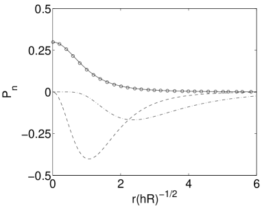
Figure 1: Functions $P_{n}\left(r\right)=p_{n}h^{2}/3\mu UR$ in series (2) for $h\ll\min\{b_{2},L\},$ $b_{1}/h=0.5$, $\phi_{2}=0.8$. Solid line corresponds to an analytical solution for $\tilde{P}=\tilde{p}h^{2}/3\mu UR$, circles - to a numerical evaluation of $P_{0}$, dashed line - to $10^{3}P_{1}$ and dash-dotted line - to $10^{5}P_{2}$.

The solution of Eq. (1) is simple if ratio $k_{\parallel}/k_{\perp}$ (and hence $\Delta k/\langle k\rangle$) is constant, i.e., when the permeabilities depend on $r$ similarly, $k_{\parallel}^{\ast},\ k_{\perp}^{\ast}\sim g\left(r\right).$ This is the case in a thin channel with $b_{1}=0$, when all the permeabilities are proportional to $H^{2}$ Feuillebois et al. (2009). Then the solution includes only axisymmetric term $p_{0}$. It can be verified directly that solution

$$\frac{d\tilde{p}}{dr}=-\frac{\mu Ur}{2H\langle k\rangle}=-\frac{12\mu Ur}{H^{3}\left(k_{\parallel}^{\ast}(H)+k_{\perp}^{\ast}(H)\right)},$$ (5)

$$\frac{\tilde{p}(H)}{12\mu UR}=\int\limits_{H}^{\infty}{\frac{dH^{\prime}}{H^{\prime}{}^{3}\left(k_{\parallel}^{\ast}+k_{\perp}^{\ast}\right)}}$$ (6)

satisfies Eq. (1) since the boundary conditionsare homogeneous, $\partial\widetilde{p}/\partial\varphi=0$, and terms

$$\frac{\partial}{\partial r}\left(H\Delta k\frac{\partial\widetilde{p}}{\partial r}\right)=\frac{\Delta k}{2\langle k\rangle}\mu U,\quad\frac{H\Delta k}{r}\frac{\partial\widetilde{p}}{\partial r}=\frac{\Delta k}{2\langle k\rangle}\mu U,$$

cancel out. The analytical expressions for $\widetilde{P}=\widetilde{p}h^{2}(3\mu UR)^{-1}$ and corresponding resistance force in the case when $h\ll\min\{b_{2},L\}$ are obtained in the Appendix section of the main paper.

The first three harmonics in series (2), plotted as functions of $r/\sqrt{hR}$, are presented in Fig. 1. It shows that the axisymmetric part of pressure distribution is very close to the approximate solution $\widetilde{P}$ while the non-axisymmetric part is several orders less.

The permeability difference is typically small, $|\Delta k|\ll|\langle k\rangle|$, for example, for large distances between surfaces, $H\gg L.$ The asymptotic solution of Eqs. (3), (4) can be found in this important case as power series expansion $P_{n}=\sum\nolimits_{j=0}\varepsilon^{j}P_{n}^{(j)}$ with respect to small parameter $\varepsilon$. We do not construct the full asymptotic solution, but show that the isotropic part $P_{0}$, which only contributes to the drag force, differs from the approximate solution $\widetilde{P}$ given by Eq. (6) by the value $O\left(\varepsilon^{2}\right).$ Substituting the expansions into the system (3), (4) and collecting the terms proportional to $\varepsilon^{j}$ one obtains equations governing the first three terms of expansion:

$$\mathrm{L}_{0}P_{0}^{(0)}=\frac{4k}{\langle k\rangle\left(0\right)}\exp\left(2\xi\right),$$ (7)

$$P_{n}^{(0)}=0\quad\text{as}\quad n>0,$$

$$\mathrm{L}_{1}P_{1}^{(1)}=-\mathrm{L}_{1}^{-}P_{0}^{(0)},$$

$$P_{n}^{(1)}=0\quad\text{as}\quad n\neq 1,$$

$$\mathrm{L}_{0}P_{0}^{(2)}=-\mathrm{L}_{0}^{+}P_{1}^{(1)},$$

$$\mathrm{L}_{2}P_{2}^{(2)}=-\mathrm{L}_{2}^{-}P_{1}^{(1)},$$

$$P_{1}^{(2)}=0,\ P_{n}^{(2)}=0\quad\text{as}\quad n>2.$$

The equation (7) is the dimensionless form of Eq. (5). For further terms, one can deduce that

$$P_{n}=\varepsilon^{n}P_{n}^{(n)}+\varepsilon^{n+2}P_{n}^{(n+2)}+\varepsilon^{n+4}P_{n}^{(n+4)}+...$$

Thus the first-order correction to the pressure field is $\varepsilon P_{1}^{(1)},$ while the correction to the isotropic part $\varepsilon^{2}P_{0}^{(2)}$ is much smaller.

References

Godunov (1961)
S. K. Godunov, Uspekhi Matematicheskikh Nauk, 1961, 16,
171–174.
Conte (1966)
S. D. Conte, SIAM Review, 1966, 8, 309.
Feuillebois et al. (2009)
F. Feuillebois, M. Z. Bazant and O. I. Vinogradova, Phys. Rev. Lett.,
2009, 102, 026001.