Enhanced CMBR non-Gaussianities from Lorentz violation

Diego Chialva
Université de Mons, Service de Mécanique et gravitation, Place du Parc 20, 7000 Mons, Belgium
diego.chialva@umons.ac.be

We study the effects of Lorentz symmetry violation on the scalar CMBR bispectrum. We deal with dispersion relations modified by higher derivative terms in a Lorentz breaking effective action and solve the equations via approximation techniques, in particular the WKB method. We quantify the degree of approximation in the computation of the bispectrum and show how the absolute and relative errors can be made small at will, making the results robust.

Our quantitative results show that there can be enhancements in the bispectrum for specific configurations in momentum space, when the modified dispersion relations violate the adiabatic condition for a short period of time in the early Universe. The kind of configurations that are enhanced and the pattern of oscillations in wavenumbers that generically appear in the bispectrum strictly depend on the form of the modified dispersion relation, and therefore on the pattern of Lorentz violation. These effects are found to be distinct from those that appear when modelling very high-energy (transplanckian) physics via modified boundary conditions (modified vacuum). In fact, under certain conditions, the enhancements are even stronger, and possibly open a door to the experimental study of Lorentz violation through these phenomena.

After providing the general formulas for the bispectrum in the presence of Lorentz violation and modified dispersion relations, we also discuss briefly a specific example based on a healthy modification of the Corley-Jacobson dispersion relation with negative coefficient, and plot the shape of the bispectrum in that case.

1 Introduction

The non-Gaussian features of the anisotropies of the Cosmic Microwave Background Radiation (CMBR) have received increasing attention in recent times, in connection with the upcoming release of the data of experiments like Planck [1]. The primordial scalar non-Gaussianity occurs when the three- and higher-point functions of the comoving curvature perturbation $\zeta$ are non-zero, and are therefore a manifestation of the interactions at the time of inflation [2]. However, they could carry signatures of physics at much higher energy, in particular of the so called transplanckian physics [3, 4].

In this work we are interested in the bispectrum, which is obtained from the three-point function, in single-field slow-roll models of inflation. In the conventional scenario this is slow-roll suppressed [2], hence any non-Gaussian signature is a smoking-gun for deviation from the standard picture. The effect one would generally be interested in for detection is a peculiar shape function, that is a specific shape for the graph of the bispectrum as a function of the external momenta, with, in particular, the presence of enhancements for some of their configurations.

There have been several approaches to the study of high energy (transplanckian) physics in cosmology: from the standard program of including higher-derivative terms in the field theory action, to the modeling via modified uncertainty relations [5], or via specific boundary conditions imposed at certain times/energy scales through boundary actions/momenta cutoffs [6, 7]. In this paper, we focus on the effects on the bispectrum due to higher-derivative corrections yielding modified dispersion relations for the perturbations fields . The dispersions differ from the Lorentzian one when the physical momenta are above a certain energy scale $\Lambda\gg H$, where $H$ is the Hubble rate at inflation [10, 11, 12].

Such effects would represent a signature of Lorentz violation at high energy and possibly open up new opportunities to study those phenomena through the CMBR. The interest in Lorentz violation has always been high [13, 14, 15, 16, 17] and revived in recent times also by certain realization of quantum gravity, such as the Hořava-Lifshitz model [18]. Lorentz violation also arises in braneworld models [19] and modified dispersion relations also appear in effective theory of single field inflation when the scalar perturbations propagate with a small sound speed [20].

In [21], the effects on the bispectrum due to modified dispersion relations which do not violate the WKB (adiabatic) condition at early times were studied via the specific example of the Corley-Jacobson dispersion relation with positive quartic correction to the momentum square term [22], where the exact solution to the field equation could be obtained. No large enhancement factors were found, but the leading modifications to the standard slow-roll results were strongly suppressed by the ratio ${H^{2}\over\Lambda^{2}}$. This can be explained in terms of the very small particle creation, due to the absence of WKB violation at early times.

In this article, we provide a more general analysis of modified dispersion relation and their effects on the bispectrum. In particular, we consider the case where the adiabatic condition is violated in the early Universe for a short period of time. In this more interesting scenario, particle production is more substantial. In fact, the Bogoljubov coefficients accounting for particle production do not depend on small ratios of energy scales such as ${H\over\Lambda}$, but, as we will show, are only constrained by backreaction. On top of that, particle creation might also lead to enhancements factors in the bispectrum for specific configurations of the three external momenta, due to interference patterns.

We will find that the leading modifications to the standard slow-roll result for the bispectrum in the presence of this kind of modified dispersion relations exhibit two main features: there appear modulations (oscillations) in function of the momenta and there can be enhancements factors for some of their configurations. We show how their presence, their magnitude and the enhanced configurations depend on, and can be obtained from, the form of the modified dispersion relation. We also find that, under certain conditions, the enhancements can be actually larger than those present within the modified vacuum framework for transplanckian physics [3], in particular when there are higher-derivative interaction terms. The reason is that in the case of modified dispersion relations some particular cancellations in the three-point function do not occur any more. We comment on the likelihood of satisfying the necessary conditions for having enhancements. We also study the backreaction issue and derive the relevant constraints descending from it.

The results are robust, as we will show that the errors deriving from the use, when necessary, of approximations to the solution of the field equation can be made small at will. Our general results can be easily adapted to the theory models of interest, obtaining from the effective action the relevant dispersion relation. In the appendix at the end of this paper, we apply our analysis to a particular example, which is a physical modification of the Corley-Jacobson relation with negative coefficient, avoiding imaginary frequencies.

The outline of the paper is as follows: we start in section 2 by introducing the formalism for describing Lorentz violation and cosmological perturbation theory, and setting the notation. We then study the modified field equation for the perturbations and its solution in section 3. Our results regarding the bispectrum are presented in section 4: in particular, in section 4.1 we study the case of pure cubic interactions and in section 4.2 the case of cubic terms with higher derivatives. We then discuss the backreaction issue and find the constraints it imposes in section 5. We conclude in section 6 with a summary and comments. Finally, the typical Lorentz-breaking action can be read in appendix A.1, and we apply our results and techniques to a specific example of modified dispersion relation in section A.2.

2 Formalism and notation.

The approaches to the implementation of Lorentz violation have been various (for reviews, see [13]). We will prefer the most conservative point of view, within the framework of Effective Field Theory and preserving general covariance and absence of fixed geometry. These latter require that Lorentz symmetry be violated by dynamical Lorentz violating tensors, which, if we preserve rotational symmetry in the dispersion relation, can be reduced to (products of) vectors [13]. Preserving general covariance is clearly appealing, because otherwise we would have to give up general relativity.

The standard procedure of cosmological perturbation theory can then be followed. It begins distinguishing background values and perturbations for the various fields. The cosmological background has a scale of variation much lower than those of the Lorentz breaking corrections, and its standard description is valid. The distinction between background and perturbations can be operated using different threadings and slicings. In [2], two gauges were used, differing in the behaviour of the comoving curvature perturbation $\zeta(\vec{x},t)$ and the inflaton perturbation $\varphi(\vec{x},t)$ (we indicate with $\phi(t)$ its background value). In one gauge

$$\zeta(\vec{x},t)=0,\qquad\varphi(\vec{x},t)\neq 0\,,$$ (1)

in the other

$$\zeta(\vec{x},t)\neq 0,\qquad\varphi(\vec{x},t)=0.$$ (2)

The latter gauge is more convenient conceptually, as one works directly with the physically interesting perturbation (the curvature one, which is conserved outside the horizon), but the former one is often better computationally.

In our case, the first gauge is by far the most convenient, as one can take into account the higher derivatives correction via the action of the inflaton (a simple scalar field). The inflaton sector will therefore be our Lorentz-breaking sector. This is especially appealing when discussing backreaction, as we will do in section 5, because one does not have to compute the effective stress-energy tensor of the metric perturbations, which is a complicate calculation. A covariant action with higher-derivative terms and a dynamical Lorentz-breaking vector field can be constructed [12, 14, 15]; we report it in appendix A.1.

The transformation between the two gauges is a time-reparametrization $t\to t+T$, such that

$$\zeta=HT+{1\over 2}H_{,t}T^{2}-{1\over 4}\partial_{i}T\partial_{j}Ta^{-2}+{1\over 2}\partial_{i}\chi\partial_{i}T+{1\over 4}a^{-2}\partial^{-2}\partial_{i}\partial_{j}\left(\partial_{i}T\partial_{j}T\right)-{1\over 2}\partial^{-2}\partial_{i}\partial_{j}\left(\partial_{i}\chi\partial_{j}T\right)$$ (3)

where $H$ and $a$ are, respectively, the Hubble rate and the metric scale factor, while

$$T=-{\varphi\over\phi_{,t}}-{1\over 2}{(\phi_{,t})_{,t}\varphi^{2}\over(\phi_{,t})^{3}}+{\varphi_{,t}\varphi\over(\phi_{,t})^{2}}\,,\qquad\partial^{2}\chi={(\phi_{,t})^{2}\over H^{2}}{d\over dt}\biggl{(}-{H\over\phi_{,t}}\varphi\biggr{)}.$$ (4)

The higher order terms in $\varphi$ and in the slow-roll parameter $\varepsilon={\dot{\phi}^{2}\over 2H^{2}M_{{}_{\text{Planck}}}^{2}}$ are necessary to compensate for the time evolution of $\varphi$ on superhorizon scales and make $\zeta$ conserved outside the horizon. For our needs, it suffices to consider this relation only at leading order in perturbations and slow roll parameters.

We expand the inflaton perturbation $\varphi$ as

$$\varphi(\eta,x)=\int{d^{3}k\over(2\pi)^{{3\over 2}}}\varphi_{{\vec{k}}}(\eta)e^{i\vec{k}\cdot\vec{x}}\,,$$ (5)

using the conformal time $\eta=\int dta^{-1}(t)$, and quantize writing

$$\varphi_{{\vec{k}}}(\eta)=f_{{\vec{k}}}(\eta)\hat{a}_{\vec{k}}^{\dagger}+f_{{\vec{k}}}^{*}(\eta)\hat{a}_{\vec{k}}\,,$$ (6)

where $f_{{\vec{k}}}(\eta),f_{{\vec{k}}}^{*}(\eta)$ are two linearly independent solutions of the field equation

$$f_{\vec{k}}^{\prime\prime}+\left(\omega(\eta,{\vec{k}})^{2}-{z^{\prime\prime}\over z}\right)f_{\vec{k}}=0\qquad z={a\phi_{,t}\over H}\,.$$ (7)

Different choices for $f_{{\vec{k}}}^{*}(\eta),f_{{\vec{k}}}(\eta)$ correspond to different choices of vacuum for the field. Imposing the standard commutation relation on the operators $\hat{a}_{{}_{\vec{k}}}~{}^{\text{\tiny$\dagger$}},\hat{a}_{{}_{\vec{k}}}$, implies a certain normalization for the Wronskian of $f_{{\vec{k}}}^{*}(\eta),f_{{\vec{k}}}(\eta)$. Using equation (3) at leading order, the comoving curvature perturbation is then expanded as

$$\zeta(\eta,x)=\int{d^{3}k\over(2\pi)^{{3\over 2}}}\zeta_{{\vec{k}}}(\eta)e^{i\vec{k}\cdot\vec{x}}\,,\qquad\zeta_{{\vec{k}}}(\eta)={\varphi_{{\vec{k}}}(\eta)\over z}\,.$$ (8)

In equation (7), $\omega(\eta,{\vec{k}})$ is the comoving frequency as read from the effective action. In the standard Lorentzian case $\omega(\eta,{\vec{k}})$ is equal to $k\equiv|{\vec{k}}|$, but for a modified dispersion relation $\omega$ will have a different dependence on ${\vec{k}},\eta$. For isotropic backgrounds, which we will limit ourselves to, $f_{{\vec{k}}}(\eta)$ and $\omega(\eta,{\vec{k}})$ depend only on $k$ and, therefore, we may drop the arrow symbol in the following.

3 Modified dispersion relations, field equations and WKB method.

We rewrite here for convenience the field equation (7) for the mode functions:

$$f_{\vec{k}}^{\prime\prime}+V(\eta,{\vec{k}})^{2}f_{\vec{k}}=0\qquad V(\eta,{\vec{k}})^{2}\equiv\omega(\eta,{\vec{k}})^{2}-{z^{\prime\prime}\over z}.$$ (9)

Solving it in the case of a modified dispersion relation is often difficult and approximation methods have to be employed. One of them consists in exploiting the WKB approximation where possible. This approach provides a global approximated solution to differential equations whose highest derivative term is multiplied by a small parameter that we call $\epsilon$ [23]. We will therefore rewrite equation (9) in such a way that the WKB method can be rigorously applied. Our approach will somehow differ from what has been done in the past in the cosmological literature discussing the spectrum of perturbations, and will enable us to have a better control on the approximation.

It is useful to start with a brief general review of the WKB method to make the paper self-contained and fix the notation; more details can be found in [23]. The method applies to equations of the form

$$\epsilon{d^{n}f\over dy^{n}}+a(y){d^{n-1}f\over dy^{n-1}}+b(y){d^{n-2}f\over dy^{n-2}}+\cdots+m(y)f=0\,,$$ (10)

but it can also be used for inhomogeneous equations, to approximate the Green functions. In our case the equations are of second order and can be put in the form

$$\epsilon^{2}{d^{2}f\over dy^{2}}+q(y)f=0$$ (11)

The WKB method consists then in:

• postulating an approximated solution of the form

  $$f(y)\sim e^{{1\over\delta}\sum_{n\geq 0}\delta^{n}s_{n}}\,,$$ (12)

  for a small parameter $\delta$ that will be fixed by studying the differential equation as we will show,

• substituting the ansatz (12) in the equation (11), obtaining

  $${\epsilon^{2}\over\delta^{2}}\dot{s}_{0}^{2}+{\epsilon^{2}\over\delta}2\dot{s}_{0}\dot{s}_{1}+{\epsilon^{2}\over\delta}\ddot{s}_{0}+\epsilon^{2}\,\dot{s}_{1}^{2}+\epsilon^{2}\,2\dot{s}_{0}\dot{s}_{2}+\epsilon^{2}\,\ddot{s}_{1}+O(\epsilon^{2}\,\delta)+q(y)=0\,,$$ (13)

• determining the value of $\delta$ through a distinguishing limit (see [23] and in the following) and solving the sequence of equations obtained from (13) by comparing powers of $\epsilon$.

We will soon give practical examples of these steps when presenting the cosmological application. Before that, let us discuss the validity conditions for the WKB approximation. The first condition is that the series at the exponent of (12) is an asymptotic series uniformly for all the interval of $x$ considered. Moreover, the validity of the procedure for solving the differential equations requires/guarantees that the series can be differentiated term-wise (at least up to the order of the equations) and the derivative series are all asymptotic as well. We then need to satisfy [23]

$$\delta s_{n+1}\sim o(s_{n})\to\biggl{|}{\delta s_{n+1}\over s_{n}}\biggr{|}\ll 1,,\qquad\delta\dot{s}_{n+1}\sim o(\dot{s}_{n})\to\biggl{|}{\delta\dot{s}_{n+1}\over\dot{s}_{n}}\biggr{|}\ll 1,\qquad\cdots\quad\forall\,n,\qquad\delta\to 0\,$$ (14)

uniformly for the interval of $x$ considered.

Furthermore, since the asymptotic series is at the exponential, these conditions are not enough to guarantee that we have a good approximation of $f(y)$: for the WKB series truncated at the order $m$ to be a good approximation of $f(y)$ we must also require

$$\delta^{m}s_{m+1}\ll 1\qquad\delta\to 0.$$ (15)

The relative error made when using the WKB approximation truncated at the order $m$ is then

$${f(y)-e^{{1\over\delta}\sum_{n=0}^{m}\delta^{n}s_{n}}\over f(y)}\sim\delta^{m}s_{m+1}\,.$$ (16)

We will also be concerned with the error done when integrating the WKB approximation in place of the exact solution. It can be found that

$$\int f(y)-\int e^{{1\over\delta}\sum_{n=0}^{m}\delta^{n}s_{n}}\sim\int e^{{1\over\delta}\sum_{n=0}^{m}\delta^{n}s_{n}}\,\delta^{m}s_{m+1}$$ (17)

$$\int f_{1}(y)f_{2}(y)f_{3}(y)-\int\prod_{i=1}^{3}e^{{1\over\delta}\sum_{n=0}^{m}\delta^{n}s_{i,n}}\sim\int\prod_{i=1}^{3}e^{{1\over\delta}\sum_{n=0}^{m}\delta^{n}s_{i,n}}\,\delta^{m}\sum_{j=1}^{3}s_{j,m+1}$$ (18)

which, beside being small because proportional to $\delta^{m}$, is further suppressed when $e^{{1\over\delta}\sum_{n=0}^{m}\delta^{n}s_{i,n}}$ is a rapidly oscillating function, as it will be in our case. These criteria are quantitative and tell us the order we need to go to for approximating the result to some prescribed error, which we can make small at will by going to higher orders in the approximation.

The conditions (14), (15) are the WKB condition(s). Given an equation of the form (11), they generically require a slow variation of the quantity $q(x)$ and are also called “adiabatic”.

Let us now investigate the application of the WKB method to the cosmological equation (9) in the case of modified dispersion relations. We will show that there is in fact a natural choice of variables such that a small parameter appears. We consider dispersion relations where the usual linear behaviour receives non-negligible corrections when the momentum is larger than a certain physical scale $\Lambda\gg H$, and therefore the dispersion relation can be written in general as 

$$\omega(\eta,k)={\omega_{{}_{\text{phys}}}(p)\over a(\eta)}={p\over a(\eta)}\;F\left(-{p\over\Lambda}\right)=k\;F\left({H\over\Lambda}k\eta\right)\,,\qquad F(x\to 0)\to 1\,.$$ (19)

We now change variable to $y=k\eta{H\over\Lambda}$ and call ${H\over\Lambda}=\epsilon$. The field equation then reads

$$\epsilon^{2}\,\ddot{f}_{y}+\biggl{(}F(y)^{2}-\epsilon^{2}{2\over y^{2}}\biggr{)}f_{y}=0\,,$$ (20)

So far, we need not specify if we discuss sub- or superhorizon scales. We proceed with the WKB method and write (13) with

$$q(y)=F(y)^{2}-\epsilon^{2}{2\over y^{2}}\,.$$ (21)

By looking at equations (13) and (21), we spot two possible distinguished limits for $\delta$, that is $\delta\sim\epsilon$ and $\delta\sim 1$. They arise from two different dominant balance conditions [23]. In the first case, the leading equation when considering powers of $\epsilon$ is

$$\dot{s}_{0}^{2}+F(y)^{2}=0$$ (22)

In the second case the leading equations are

$$\epsilon^{2}\biggl{(}(\sum_{n}\dot{s}_{n})^{2}+\sum_{n}\ddot{s}_{n}-{2\over y^{2}}\biggr{)}=0\qquad F(y)^{2}\ll\epsilon^{2}{2\over y^{2}}$$ (23)

Here, it surfaces the distinction between superHubble and subHubble modes, which corresponds respectively to the first and second distinguished limit for $\delta$. In section 3.1, we will use the WKB approximation in the intervals of time where the first limit is appropriate, and look for a different solution in the case of the second limit. In fact, in this latter case, the WKB conditions (14), (15) will not be satisfied .

For the moment, let us discuss which kind of modified dispersion relations can appear. In general, they can be divided in two different classes, on the basis of the behaviour of the frequency at early times and the value of the Bogoljubov parameters.

The first class is represented by those dispersion relations for which there is no violation of the WKB condition at early times, but only at very late times when the dispersion has the linear form $\omega\approx k$ as in the standard case. A good example within this class is the Corley-Jacobson relation with positive coefficients [22], which was studied in [21]. In this case, the WKB approximation (well-suited for these relations) shows that the corrections to the spectrum and bispectrum are very suppressed.

The second class of dispersion relations consists instead of those violating the WKB (adiabatic) condition at early times. This scenario is more promising: first, interference terms will generally appear in the bispectrum due to the presence of both positive and negative frequency solutions in consequence of the early WKB violation. In this case, one could therefore expect large enhancement factors for some configurations because of interference and phase cancellation. Second, the Bogoljubov coefficients indicating particle creation are actually quite independent of any ratio of scales of the form ${H\over\Lambda}$, as we will show, and are proportional to the parameter signalling the WKB violation and the interval of time during which the WKB approximation is not good. The only constraint is due to the request of small backreaction [11].

In the following, we will study the corrections to the bispectrum for dispersion relations with the behaviour represented in figure 1, where the WKB condition is violated at early times. The times $\eta_{\mbox{\text{{\tiny{\rm I}}}}},\eta_{\mbox{\text{{\tiny{\rm I}}}\text{{\tiny{\rm I}}}}},\eta_{\mbox{\text{{\tiny{\rm I}}}\text{{\tiny{\rm I}}}\text{{\tiny{\rm I}}}}}$ signalling the transition between violated/satisfied WKB condition are individuated by the violation of (some of) the conditions in equations (14), (15), and are close to the turning points $\eta_{1},\eta_{2},\eta_{3}$ in figure 1. They are inversely proportional to the wavenumber $k$, being given by a condition on $y=\epsilon k\eta$, and hence, more correctly, we will indicate them with the notation $\eta^{(k)}_{j}$ when necessary to avoid confusion. It is important that at very late times the WKB condition (adiabaticity) is restored, because in that case we can unambiguously determine a vacuum state and fix initial data. We will also briefly comment on the case of dispersion relations with no WKB violation at early times, generalizing the results found in [21].

Dispersion relations that are more complicated than the one in figure 1 can be imagined, with several period of WKB violation and a more varied behaviour, but the analysis in those cases amounts to repeating the one we do for the case in figure 1 in the various regions of WKB validity or violation.

Figure 1: Dispersion relation with violation of WKB at early times.

3.1 Solving the field equations

In the case of a dispersion relation like the one in figure 1, the time axis can be divided in four regions, and the solution written as follows

$$f_{\vec{k}}(\eta)=\begin{cases}\varsigma_{\vec{k}}\,u_{1}(\eta,{\vec{k}})&\qquad{\rm I}:\;\eta<\eta^{(k)}_{\mbox{\text{{\tiny{\rm I}}}}}\\ B_{1}\,\mathcal{U}_{1}(\eta,{\vec{k}})+B_{2}\,\mathcal{U}_{2}(\eta,{\vec{k}})&\qquad{\rm II}:\;\eta^{(k)}_{\mbox{\text{{\tiny{\rm I}}}}}<\eta<\eta^{(k)}_{\mbox{\text{{\tiny{\rm I}}}\text{{\tiny{\rm I}}}}}\\ \alpha_{\vec{k}}\,u_{1}(\eta,{\vec{k}})+\beta_{\vec{k}}\,u_{2}(\eta,{\vec{k}})&\qquad{\rm III}:\;\eta^{(k)}_{\mbox{\text{{\tiny{\rm I}}}\text{{\tiny{\rm I}}}}}<\eta<\eta^{(k)}_{\mbox{\text{{\tiny{\rm I}}}\text{{\tiny{\rm I}}}\text{{\tiny{\rm I}}}}}\\ D_{1}\,\mathcal{V}_{1}(\eta,{\vec{k}})+D_{2}\,\mathcal{V}_{2}(\eta,{\vec{k}})&\qquad{\rm IV}:\;\eta^{(k)}_{\mbox{\text{{\tiny{\rm I}}}\text{{\tiny{\rm I}}}\text{{\tiny{\rm I}}}}}<\eta\end{cases}$$ (24)

The coefficients $\alpha_{\vec{k}},\beta_{\vec{k}},B_{1,2},D_{1,2}$ are determined by imposing continuity for the function and its first derivative, $\varsigma_{\vec{k}}$ is determined by the choice of boundary conditions for $\eta\to-\infty$.

We also must impose the Wronskian condition $\mathcal{W}\{f,f^{*}\}=-i$ to have the standard commutation relations in the quantum theory. If we impose it at a certain time, the continuity of the function and its first derivative ensures that it will be always satisfied because of Abel’s theorem and equation (9).

The partial solutions listed in equation (24) will be presented in the next sections; in particular, we will use the WKB method to obtain $u_{1,2}$ and choose the adiabatic vacuum for the field.

3.1.1 The WKB solution of the field equations in regions I and III

As we have shown, the WKB method has lead us to the equation (13) with $q(y)$ given by (21), which can be solved in sequence comparing powers of $\epsilon$. In the regions I, III the correct distinguished limit is $\delta\sim\epsilon$, leading to the sequence

$$\begin{cases}\dot{s}_{0}^{2}+F(y)^{2}=0\\ 2\dot{s}_{0}\dot{s}_{1}+\ddot{s}_{0}=0\\ \dot{s}_{1}^{2}+2\dot{s}_{0}\dot{s}_{2}+\ddot{s}_{1}-{2\over x^{2}}=0\\ 2\dot{s}_{1}\dot{s}_{2}+2\dot{s}_{0}\dot{s}_{3}+\ddot{s}_{2}=0\\ \cdots\end{cases}\,.$$ (25)

To take into account the ${z^{\prime\prime}\over z}$ term in the field equation, we need to include up to the order $\delta^{2}$ in the series expansion for the WKB solution. The Wronskian condition then forces us to consider also the order $\delta^{3}$. In this way we obtain the positive- and negative-frequency WKB solutions $u_{1,2}$

$$u_{1}(y_{k})={e^{-{i\over\epsilon}\Omega(y_{k})}\over\sqrt{2\,k\,U(y_{k})}}\,,\qquad u_{2}(y_{k})=u_{1}^{*}(y_{k})={e^{+{i\over\epsilon}\Omega(y_{k})}\over\sqrt{2\,k\,U(y_{k})}}\,,$$ (26)

$$\Omega(y_{k})=\int^{y_{k}}U(y^{\prime}_{k})dy^{\prime}_{k}\,,\qquad U(y_{k})\equiv S_{0}+\epsilon^{2}S_{2}\equiv F+\epsilon^{2}\biggl{(}-{\ddot{F}\over 4F^{2}}+3{(\dot{F})^{2}\over 8F^{3}}-{1\over Fy_{k}^{2}}\biggr{)}\,.$$ (27)

With the above notation for $\Omega(y_{k})$ we intend the primitive of $U$ evaluated at $y_{k}=\epsilon k\eta$, since we absorb the phases resulting from the lower limit of integration in the coefficients $\varsigma_{\vec{k}},\alpha_{\vec{k}},\beta_{\vec{k}}$. The notation $y_{k}$ keeps track of the $k$-dependence of the definition of $y$ and will be useful in the following. We have also normalized the solution with a factor $\sqrt{k}^{-1}$ because in this way the Wronskian constraint $\mathcal{W}\{u_{1},u_{2}\}=-i$ in the $\eta$-coordinate is solved if $\varsigma_{\vec{k}}$ is a pure phase, and $|\alpha_{\vec{k}}|^{2}-|\beta_{\vec{k}}|^{2}=1$.

The WKB approximation is good when all the conditions (14), (15) are satisfied. In particular, since we truncated the series at the order $\delta^{3}$, we must require, among the other conditions,

$$\epsilon^{4}\biggl{|}{\dot{s}_{4}\over\dot{s}_{0}}\biggr{|}\ll 1\,.$$ (28)

Observe that, by direct derivation, our WKB solutions are found to precisely satisfy the equation (using the coordinate $\eta$)

$$u_{1,2}^{\prime\prime}+\bigl{[}V(\eta,{\vec{k}})^{2}-\mathcal{Q}(\eta,{\vec{k}})\bigr{]}u_{1,2}=0$$ (29)

where

$$\mathcal{Q}=-\biggl{(}-{\omega^{\prime\prime}\over 4\omega^{2}}+3{\omega^{{}^{\prime}2}\over 8\omega^{3}}-{1\over\omega y^{2}}\biggr{)}^{2}+{\omega^{\prime\prime}\over 2\omega}-3{\omega^{{}^{\prime}2}\over 4\omega^{2}}-{U^{\prime\prime}\over 2U}+3{U^{{}^{\prime}2}\over 4U^{2}}\underset{\eta\to y_{k}}{\simeq}-\epsilon^{4}2\dot{s}_{0}(y_{k})\dot{s}_{4}(y_{k})\,,$$ (30)

therefore the condition (28) corresponds to $\bigl{|}{\mathcal{Q}\over V^{2}}\bigr{|}\ll 1$. The times $\eta_{\mbox{\text{{\tiny{\rm I}}}\text{{\tiny{\rm I}}}}},\eta_{\mbox{\text{{\tiny{\rm I}}}\text{{\tiny{\rm I}}}\text{{\tiny{\rm I}}}}}$ are then such that $\bigl{|}{\mathcal{Q}\over V^{2}}\bigr{|}_{\eta_{\mbox{\text{{\tiny{\rm I}}}\text{{\tiny{\rm I}}}},\mbox{\text{{\tiny{\rm I}}}\text{{\tiny{\rm I}}}\text{{\tiny{\rm I}}}}}}\not\ll 1$.

3.1.2 The solution of the field equations in regions II and IV

The WKB approximation is not good in the regions II and IV . In previous works, then, it has then often been taken the drastic approximation that $V(\eta,{\vec{k}})^{2}\approx{z^{{}^{\prime\prime}}\over z}$ in those regions, so that the solution of equation (9) reduced to a growing and decaying mode depending on the scale factor. For the purpose of studying the bispectrum, we employ more refined and accurate approximations.

Indeed, in region IV, when $\eta>\eta_{\mbox{\text{{\tiny{\rm I}}}\text{{\tiny{\rm I}}}\text{{\tiny{\rm I}}}}}$, the dispersion relation is in the linear regime

$$\omega^{2}(\eta>\eta_{\mbox{\text{{\tiny{\rm I}}}\text{{\tiny{\rm I}}}\text{{\tiny{\rm I}}}}},{\vec{k}})=k^{2},$$ (31)

and the solution is given in terms of the Hankel functions $\mathcal{V}_{1,2}=\sqrt{-\eta}H^{(1,2)}_{\nu}(-k\eta),\;\nu\sim{3\over 2}$. By asking for the continuity of the function and its first derivative at $\eta\lesssim\eta_{\mbox{\text{{\tiny{\rm I}}}\text{{\tiny{\rm I}}}\text{{\tiny{\rm I}}}}}$, we find that

$$D_{1}={\sqrt{\pi}\over 2}e^{i{\pi\over 2}\nu+i{\pi\over 4}}\alpha_{\vec{k}}\qquad D_{2}={\sqrt{\pi}\over 2}e^{-i{\pi\over 2}\nu-i{\pi\over 4}}\beta_{\vec{k}}$$ (32)

When instead $\eta_{\mbox{\text{{\tiny{\rm I}}}}}<\eta<\eta_{\mbox{\text{{\tiny{\rm I}}}\text{{\tiny{\rm I}}}}}$, in region II, we indicate with $\mathcal{U}_{1,2}(k,\eta)$ the solutions obtained not neglecting the $\omega^{2}$ term in the potential $V^{2}$ in equation (9). Actually, we will find that some of the important features of the bispectrum can be found without knowing the details of the field solution, but just using the fact that small backreaction requires having a short interval $[\eta_{\mbox{\text{{\tiny{\rm I}}}}},\eta_{\mbox{\text{{\tiny{\rm I}}}\text{{\tiny{\rm I}}}}}]$, as we will show in section 5. In this sense, those results will be very robust, being independent of the approximations chosen when solving the field equations.

When needed, however, a rather accurate approximation in region II is obtained observing that, given figure 1, the physical frequency has a local minimum $\omega_{0}$ at $\eta=\eta_{m}$, and therefore

$$\omega^{2}=a^{2}\omega_{{}_{\text{phys}}}^{2}\simeq{1\over\eta^{2}H^{2}}\biggl{(}\omega_{0}^{2}+\omega_{0}\omega_{{}_{\text{phys}}}^{{}^{\prime\prime}}(\eta_{m})(\eta-\eta_{m})^{2}\biggr{)}\,.$$ (33)

This approximation is well-justified also because, as we said, backreaction constraints the interval $[\eta_{\mbox{\text{{\tiny{\rm I}}}}},\eta_{\mbox{\text{{\tiny{\rm I}}}\text{{\tiny{\rm I}}}}}]$ to be very small, and therefore $\eta\sim\eta_{m}$ for $\eta,\eta_{m}\in[\eta_{\mbox{\text{{\tiny{\rm I}}}}},\eta_{\mbox{\text{{\tiny{\rm I}}}\text{{\tiny{\rm I}}}}}]$, see section 5 for a proof. Substituting (33) in (9), the solution is readily found:

$$f_{\vec{k}}(\eta)=B_{1}\;W(i\kappa\,\eta_{m},\sigma,2i\kappa\,\eta)+B_{2}\;W(-i\kappa\,\eta_{m},\sigma,-2i\kappa\,\eta)$$

$$\kappa\equiv{\sqrt{\omega_{0}\omega_{{}_{\text{phys}}}^{{}^{\prime\prime}}(\eta_{m})}\over H}\qquad\sigma\equiv{\sqrt{9H^{2}-4\omega_{0}^{2}-4H^{2}\kappa^{2}\eta_{m}^{2}}\over 2H}\,,$$ (34)

where $W(a,b,z)$ is the Whittacker function.

3.1.3 Initial conditions, the Bogoljubov coefficients $\alpha_{\vec{k}},\beta_{\vec{k}},B_{1},B_{2}$ and particle creation.

The result regarding the coefficients $\alpha_{\vec{k}},\beta_{\vec{k}},B_{1},B_{2}$ in (24) is robust, because it is independent of whatever assumption is made about the behaviour of $\omega$, in particular, of the form of $\omega$ assumed in equation (33). The only information we need is that the interval $[\eta_{\mbox{\text{{\tiny{\rm I}}}}},\eta_{\mbox{\text{{\tiny{\rm I}}}\text{{\tiny{\rm I}}}}}]$ is very small because of backreaction (see section 5) so that

$$\Delta={\eta_{\mbox{\text{{\tiny{\rm I}}}}}-\eta_{\mbox{\text{{\tiny{\rm I}}}\text{{\tiny{\rm I}}}}}\over\eta_{\mbox{\text{{\tiny{\rm I}}}}}}\ll 1\,,$$ (35)

and that the WKB solutions satisfy the equation (29), while the partial solutions $\mathcal{U}_{1,2}$ satisfy

$$\mathcal{U}_{1,2}^{\prime\prime}+V(\eta,{\vec{k}})^{2}\mathcal{U}_{1,2}=0\qquad\eta\in[\eta_{\mbox{\text{{\tiny{\rm I}}}}},\eta_{\mbox{\text{{\tiny{\rm I}}}\text{{\tiny{\rm I}}}}}]\,.$$ (36)

By asking for the continuity of the solution and its first derivative, we obtain in full generality

$$B_{1} ={\mathcal{W}\{\varsigma_{\vec{k}}\,u_{1},\mathcal{U}_{2}\}\over\mathcal{W}\{\mathcal{U}_{1},\mathcal{U}_{2}\}}\biggr{|}_{\eta_{\mbox{\text{{\tiny{\rm I}}}}}} B_{2} =-{\mathcal{W}\{\varsigma_{\vec{k}}\,u_{1},\mathcal{U}_{1}\}\over\mathcal{W}\{\mathcal{U}_{1},\mathcal{U}_{2}\}}\biggr{|}_{\eta_{\mbox{\text{{\tiny{\rm I}}}}}}$$ (37)

$$\alpha_{\vec{k}} ={\mathcal{W}\{B_{1}\,\mathcal{U}_{1}+B_{2}\,\mathcal{U}_{2},u_{2}\}\over\mathcal{W}\{u_{1},u_{2}\}}\biggr{|}_{\eta_{\mbox{\text{{\tiny{\rm I}}}\text{{\tiny{\rm I}}}}}} \beta_{\vec{k}} =-{\mathcal{W}\{B_{1}\,\mathcal{U}_{1}+B_{2}\,\mathcal{U}_{2},u_{1}\}\over\mathcal{W}\{u_{1},u_{2}\}}\biggr{|}_{\eta_{\mbox{\text{{\tiny{\rm I}}}\text{{\tiny{\rm I}}}}}}\,,$$ (38)

where $\mathcal{W}$ is the Wronskian. By expanding for small $\Delta$ around $\eta_{\mbox{\text{{\tiny{\rm I}}}}}$, we obtain (again, in full generality)

$$\alpha_{\vec{k}}=\biggl{(}1-i{V(\eta_{\mbox{\text{{\tiny{\rm I}}}}},k)\,\eta_{\mbox{\text{{\tiny{\rm I}}}}}\over 2}{\mathcal{Q}\over V^{2}}\biggr{|}_{\eta_{\mbox{\text{{\tiny{\rm I}}}}}}\Delta+O(\Delta^{2})\biggr{)}\,\varsigma_{\vec{k}}\,,\qquad\beta_{\vec{k}}=\biggl{(}i{V(\eta_{\mbox{\text{{\tiny{\rm I}}}}},k)\,\eta_{\mbox{\text{{\tiny{\rm I}}}}}\over 2}{\mathcal{Q}\over V^{2}}\biggr{|}_{\eta_{\mbox{\text{{\tiny{\rm I}}}}}}\Delta+O(\Delta^{2})\biggr{)}e^{-{2i\over\epsilon}\Omega_{|_{\eta_{{}_{\mbox{\text{{\tiny{\rm I}}}}}}}}}\,\varsigma_{\vec{k}}\,,$$ (39)

We see that at leading order $\beta_{\vec{k}}$ is not proportional to small ratios of scales such as ${H\over\Lambda}$, but to the parameter ${\mathcal{Q}\over V^{2}}\bigr{|}_{\eta_{\mbox{\text{{\tiny{\rm I}}}}}}$ signalling the WKB violation (see equation (30)) and the ratio $\Delta$. The only constraint to the value of $\beta_{\vec{k}}$ is therefore due to the request of small backreaction.

The Bogoljubov coefficients also depend on the choice of initial conditions, that is on the pure phase $\varsigma_{\vec{k}}$. The bispectrum will be affected by this choice as well, differently from the spectrum, where only the modulus square of the mode functions enter the computation and therefore $|\varsigma_{\vec{k}}|=1$. In the following, we will choose $\varsigma_{\vec{k}}=1$.

4 Bispectrum and modifications to the Bunch-Davies result

The three-point function for the comoving curvature perturbation can be computed in the $\varphi\neq 0$ gauge and then transformed in the $\zeta\neq 0$ gauge, using equation (3) at leading order. In the following, when we write a formula in terms of $\zeta\neq 0$ it must therefore be intended that the computation is performed in the $\varphi\neq 0$ gauge and then transformed in the $\zeta\neq 0$ one, where the quantities relevant for observation are more easily read.

In the in-in formalism, one obtains at leading order [2]

$$\langle\zeta(x_{1})\zeta(x_{2})\zeta(x_{3})\rangle=-2\text{Re}\left(\int^{\eta}_{\eta_{\text{in}}}d\eta^{\prime}i\langle\psi_{\text{in}}|\zeta(x_{1})\zeta(x_{2})\zeta(x_{3})H_{(I)}(\eta^{\prime})|\psi_{\text{in}}\rangle\right)$$ (40)

where $H_{(I)}$ is the interaction Hamiltonian, while ${\eta_{\text{in}}}$, $|\psi_{\text{in}}\rangle$ are the initial conformal time and state (vacuum). The standard result in slow-roll inflation is obtained by choosing $|\psi_{\text{in}}\rangle$ to be the Bunch-Davies vacuum and ${\eta_{\text{in}}}=-\infty$ [2].

The basic correlator in perturbation theory is given by the Whightman function

$$\langle\zeta(\eta)\zeta(\eta^{\prime})\rangle=G_{{\vec{k}}}(\eta,\eta^{\prime})\equiv{H^{2}\over\phi_{,t}\!^{2}}\frac{f_{k}(\eta)}{a(\eta)}\frac{f_{k}^{\ast}(\eta^{\prime})}{a(\eta^{\prime})}$$ (41)

We write the bispectrum as [25]

$$\langle\zeta_{{\vec{k}}_{1}}(\eta)\zeta_{{\vec{k}}_{2}}(\eta)\zeta_{{\vec{k}}_{3}}(\eta)\rangle=\hat{F}({\vec{k}}_{1},{\vec{k}}_{2},{\vec{k}}_{3},\eta)=(2\pi)^{3}\delta(\sum_{i}{\vec{k}}_{i})\hat{B}({\vec{k}}_{1},{\vec{k}}_{2},{\vec{k}}_{3},\eta)\,.$$ (42)

Scale-invariance requires the function $\hat{B}$ to be homogeneous of degree $-6$ and rotational invariance makes it a function of only two variables, which can be taken as $x_{2}\equiv{k_{2}\over k_{1}}$ and $x_{3}\equiv{k_{3}\over k_{1}}$. The conservation of momentum, with the triangle inequality, forces $x_{2}+x_{3}\geq 1$. Because of the symmetry in $x_{2}$ and $x_{3}$, it can be further assumed that $x_{3}\leq x_{2}$.

Typical configurations in the standard slow-roll/chaotic models are the local one, where $x_{3}\simeq 0$ and $x_{2}\simeq 1$, and the equilateral, where $x_{2}\simeq x_{3}\simeq 1$. The standard inflationary model with Bunch-Davies vacuum state tends to produce non-Gaussianities when the modes cross the horizon, leading to a three-point function maximized on the equilateral configuration. If instead the non-Gaussianites receive a contribution also during the superhorizon evolution, as for example in the curvaton scenario, they will tend to be maximum on a more local type of configurations [25].

In the next two sections we compute the three-point function for two cases of interactions: a cubic coupling without higher power of derivatives acting on the fields, and a cubic interaction with higher derivatives. Some of the details of the computation apply to both cases, and we discuss them at length within the former. We then use that knowledge to analyze the latter one, which will turn out to be the most interesting for observations.

4.1 Cubic scalar interactions

The interacting Hamiltonian at cubic order in the perturbations can be obtained by expanding the Einstein-Hilbert action on the quasi de Sitter background [2]. The contributions to the correlator (40) include a connected and some disconnected parts depending on how we define the curvature perturbation (that is, if we use non-linear field redefinitions). We will be using a redefinition leading to the simplest form of the cubic interaction [2]:

$$H_{(I)}=-\int d^{3}x\,a^{3}\,({\phi_{,t}\over H})^{4}\,{H\over M_{{}_{\text{Planck}}}^{2}}\,\zeta^{\prime 2}\partial^{-2}\zeta^{\prime}\,,$$ (43)

and will be interested in the connected three-point function. In the following, we indicate with the terms “three-point function” and “bispectrum” their connected parts.

Using equation (43), the three-point function (40) becomes, in momentum space,

$$\!\!\!\!\langle\zeta_{{\vec{k}}_{1}}(\eta)\zeta_{{\vec{k}}_{2}}(\eta)\zeta_{{\vec{k}}_{3}}(\eta)\rangle\!=\!2\text{Re}\biggl{(}\!-i(2\pi)^{3}\delta(\sum_{i}{\vec{k}}_{i})\biggl{(}{\phi_{,t}\over H}\biggr{)}^{4}\!\!{H\over M_{{}_{\text{Planck}}}^{2}}\!\!\int^{\eta}_{\eta_{\text{in}}}d\eta^{\prime}{{a(\eta^{\prime})^{3}}\over k_{3}^{2}}\prod_{i=1}^{3}\partial_{\eta^{\prime}}G_{{\vec{k}}_{i}}(\eta,\eta^{\prime})+\text{permutations}\!\biggr{)},$$ (44)

where $\eta$ is a late time when all modes $k_{i}$ are outside the horizon after the modified dispersion relation has become effectively the standard linear one.

Evaluated using equations (24), (32) at the late time $|\eta|\ll 1$, when all three mode functions have exited from the horizon in region IV, the Green function reads

$$\partial_{\eta^{\prime}}G_{\vec{k}}(\eta,\eta^{\prime})={H^{2}\over\phi_{,t}^{2}}{e^{i{\pi\over 2}}\over\sqrt{2}}{H\over k^{3\over 2}}(\alpha_{\vec{k}}-\beta_{\vec{k}})\,\biggl{(}{f^{*}_{\vec{k}}(\eta^{\prime})\over a(\eta^{\prime})}\biggr{)}^{\prime}\simeq{H^{2}\over\phi_{,t}^{2}}{e^{i{\pi\over 2}}\over\sqrt{2}}{H\over k^{3\over 2}}\,\biggl{(}{f^{*}_{\vec{k}}(\eta^{\prime})\over a(\eta^{\prime})}\biggr{)}^{\prime}\,.$$ (45)

To compute the bispectrum, one needs to divide up the interval of time integration in equation (44) into the different regions of validity of the piecewise solution (24) and compute the various terms. The number of terms is elevated, but many of them are identical up to permutation of the external momenta and therefore we can reduce them to some common classes which we now study. By the shortcut expression “being in region X” referred to a Green function depending on $k_{i}$, we will mean that for those values of $\eta^{\prime},k_{i}$ the function $f_{k_{i}}(\eta^{\prime})$ entering equation (45) is the partial solution of the field equation valid in region X, as shown in equation (24).

4.1.1 All Green functions in region III

We start from the analysis of the contribution to the bispectrum (44) when all the three Green functions $G_{\vec{k}}$ are in region III, which, as we will show, leads to the largest enhancements. In that region, the function in (45) has the form

$$\partial_{\eta^{\prime}}G_{\vec{k}}(\eta,\eta^{\prime})=\partial_{\eta^{\prime}}G_{\vec{k}}^{(\alpha)}(\eta,\eta^{\prime})+\partial_{\eta^{\prime}}G_{\vec{k}}^{(\beta)}(\eta,\eta^{\prime})\,,$$ (46)

where we have distinguished the positive- and negative-frequency branches $u_{1,2}(k,\eta)$ of the solution in region III, see equation (24).

There are therefore two possible contributions to the three-point function: one where the three Whightman function are all in the same positive or negative branch of the solutions, the other where one of them is in the opposite branch. It is convenient to concentrate first on the latter case.

The leading contribution in powers of $\beta_{\vec{k}}$ to the standard slow-roll result is then

$$\hat{F}_{3,\beta} =-2\text{Re}\biggl{[}-i(2\pi)^{3}\delta(\sum_{i}{\vec{k}}_{i}){H^{2}\over\phi_{,t}^{2}}{H\over M_{{}_{\text{Planck}}}^{2}}\int^{\eta^{\prime}_{\mbox{\text{{\tiny{\rm I}}}\text{{\tiny{\rm I}}}\text{{\tiny{\rm I}}}}}}_{\eta^{\prime}_{\mbox{\text{{\tiny{\rm I}}}\text{{\tiny{\rm I}}}}}}d\eta^{\prime}{1\over k_{l}^{2}}{e^{i{3\pi\over 2}}H^{3}\over\prod_{i=1}^{3}(2\,k_{i})}\beta_{{\vec{k}}_{j}}^{*}\prod_{h\neq j}\gamma^{*}({\vec{k}}_{h},\eta^{\prime})\gamma({\vec{k}}_{j},\eta^{\prime})$$

$$\qquad\qquad\qquad\qquad\times\,e^{i{\Lambda\over H}\bigl{(}\Omega(\eta^{\prime};k_{h})-\Omega(\eta^{\prime};k_{j})\bigr{)}}\biggr{]}+\text{permutations}\qquad h,j\in\{1,2,3\}\,.$$ (47)

The Green function depending on $k_{j}$ is in its negative-frequency branch, and those depending on $k_{h},\,h\neq j$ are in their positive-frequency one. The limits of integration $\eta^{\prime}_{\mbox{\text{{\tiny{\rm I}}}\text{{\tiny{\rm I}}}}},\eta^{\prime}_{\mbox{\text{{\tiny{\rm I}}}\text{{\tiny{\rm I}}}\text{{\tiny{\rm I}}}}}$ are given, respectively, by the largest and the smallest among $\eta_{\mbox{\text{{\tiny{\rm I}}}\text{{\tiny{\rm I}}}}}^{(k_{i})}$ and $\eta_{\mbox{\text{{\tiny{\rm I}}}\text{{\tiny{\rm I}}}\text{{\tiny{\rm I}}}}}^{(k_{i})}$, $i=1,2,3$. We have also defined

$$\gamma({\vec{k}},\eta)={1\over\sqrt{U}}\biggl{(}{1\over 2k}{U^{\prime}\over U}+iU+{\mathcal{H}\over k}\biggr{)}\,,$$ (48)

and the functions $U(\eta^{\prime},k)=U(y_{k}(\eta^{\prime}))$ and $\Omega(\eta^{\prime},k)=\Omega(y_{k}(\eta^{\prime}))$ are given in equation (27). $\mathcal{H}$ is the Hubble rate in conformal time, $M_{{}_{\text{Planck}}}$ is the reduced Planck mass.

We rewrite (4.1.1) as

$$\hat{F}_{3,\beta}(k_{1},k_{2},k_{3})=A\;\delta\hat{F}_{3,\beta}(k_{1},k_{2},k_{3})$$ (49)

where we factorize the amplitude, including the overall scale dependence,

$$A=4(2\pi)^{3}\delta(\sum_{i}{\vec{k}}_{i}){H^{6}\over\phi_{,t}^{2}M_{{}_{\text{Planck}}}^{2}}{k_{1}^{2}k_{2}^{2}k_{3}^{2}\over\prod_{i=1}^{3}(2k_{i}^{3})}\sum_{l}{1\over k_{t}k_{l}^{2}}\,,\qquad k_{t}=\sum_{i=1}^{3}k_{i}\,,$$ (50)

while

$$\delta\hat{F}_{3,\beta}(k_{1},k_{2},k_{3})=\sum_{j}\text{Re}\biggl{[}{\beta_{{\vec{k}}_{j}}^{*}\over 2}\int^{\eta_{\mbox{\text{{\tiny{\rm I}}}\text{{\tiny{\rm I}}}\text{{\tiny{\rm I}}}}}}_{\eta_{\mbox{\text{{\tiny{\rm I}}}\text{{\tiny{\rm I}}}}}}d\eta^{\prime}k_{t}\prod_{h\neq j}\gamma^{*}({\vec{k}}_{h},\eta^{\prime})\gamma({\vec{k}}_{j},\eta^{\prime})\,e^{i{\Lambda\over H}\bigl{(}\Omega(\eta^{\prime},k_{h})-\Omega(\eta^{\prime},k_{j})\bigr{)}}\biggr{]}\,,$$ (51)

The amplitude $A$ is precisely the standard slow-roll result [2], hence $\delta\hat{F}_{3,\beta}$ is the putative enhancement factor, to which we now turn. Recall that the modified dispersion relation implies that the frequency $\omega(\eta,k)$ depends on $k,\eta$ and the scale of new physics $\Lambda$ as in equation (19). We then change the variable $\eta^{\prime}$ in the integral in equation (51) to

$$y={H\over\Lambda}k_{{}_{\text{max}}}\eta^{\prime}\,,\qquad k_{{}_{\text{max}}}\equiv\text{max}(k_{1},k_{2},k_{3})$$ (52)

so that equation (51) reads

$$\delta\hat{F}_{3,\beta}(x_{1}=1,x_{2},x_{3})=\sum_{j}\text{Re}\biggl{[}{\beta_{{\vec{k}}_{j}}^{*}\over 2}{\Lambda\over H}x_{t}\int^{y_{\mbox{\text{{\tiny{\rm I}}}\text{{\tiny{\rm I}}}\text{{\tiny{\rm I}}}}}}_{y_{\mbox{\text{{\tiny{\rm I}}}\text{{\tiny{\rm I}}}}}}dy\prod_{h\neq j}\gamma^{*}(x_{h},y)\gamma(x_{j},y)\,e^{i{\Lambda\over H}S_{\beta}(x_{1},x_{2},x_{3},y)}\biggr{]},$$ (53)

where we have assumed, for instance, $k_{1}=k_{{}_{\text{max}}}$ and recovered the usual bispectrum variables $x_{i}={k_{i}\over k_{{}_{\text{max}}}}$ introduced at the end of section 2. To write the formulas in a more symmetric way, here and in the following, we also indicate formally the ratio $x_{1}={k_{1}\over k_{{}_{\text{max}}}}$, although it is equal to 1 because of our assumption.

We have also defined

$$S_{\beta}(x_{1},x_{2},x_{3},y)\equiv\sum_{h\neq j}\Omega(y,x_{h})-\Omega(y,x_{j})\equiv S_{0\beta}(\{x\},y)+{H^{2}\over\Lambda^{2}}S_{2\beta}(\{x\},y)$$ (54)

$$S_{0(2)\beta}(\{x\},y)=\sum_{h\neq j}S_{0(2)}(x_{h},y)-S_{0(2)}(x_{j},y)\,.$$ (55)

where the dependence of $\Omega$ on $x_{i},y$ is due to the fact that $y_{k_{i}}(\eta^{\prime})\equiv k_{i}\epsilon\eta^{\prime}=x_{i}\,y$, see equation (27), and $S_{0},S_{2}$ are the quantities appearing in the second equation in (27).

The limits of integration in (53) are computed as the values for which the WKB conditions are violated. In general, one finds that $y_{\mbox{\text{{\tiny{\rm I}}}\text{{\tiny{\rm I}}}}}={H\over\Lambda}k_{{}_{\text{max}}}\eta^{(k_{\text{max}})}_{\mbox{\text{{\tiny{\rm I}}}\text{{\tiny{\rm I}}}}}\sim-1$, since the corrections to the linear dispersion relation at the time $\eta_{\mbox{\text{{\tiny{\rm I}}}\text{{\tiny{\rm I}}}}}$ must be quite important in order to drive the frequency close to the turning point (see figure 1), and therefore looking at (19) it must be ${p_{\text{max}}\over\Lambda}\sim 1$. The upper limit is instead $y_{\mbox{\text{{\tiny{\rm I}}}\text{{\tiny{\rm I}}}\text{{\tiny{\rm I}}}}}={H\over\Lambda}k_{{}_{\text{max}}}\eta^{(k_{\text{min}})}_{\mbox{\text{{\tiny{\rm I}}}\text{{\tiny{\rm I}}}\text{{\tiny{\rm I}}}}}\sim-{H\over\Lambda}{1\over x_{{}_{k_{\text{min}}}}}$.

Evidently, the contribution (53) is sizable if the interval of integration is sufficiently large. We are therefore interested in this case, hence we will consider $x_{{}_{k_{\text{min}}}}\gtrsim 10\epsilon$, which however for $\epsilon$ reasonably small leaves plenty of room for all the values of the wavenumber relevant for the CMBR observations (consider for example that already for the supersymmetric GUT scale, it is $\epsilon\lesssim 10^{-3}$ if $H\sim 10^{-5}M_{P}$).

The integral in (53) is a typical Fourier integral which can be well approximated by the technique of stationary phase, since ${\Lambda\over H}\gg 1$ [26]. As it is known, its approximated solution depends on the critical points of $S_{0\beta}(\{x\},y)$ as a function of $y$. Their presence and nature depend on the configuration of the external momenta $k_{1,2,3}$, which act as parameters in the function.

We call stationary point of order $n-1$ an interior point $y_{*}$ such that

$$\partial_{y}^{n}S_{0\beta}(\{x\},y)|_{y=y_{*}}\equiv S_{0\beta}^{(n)}(\{x\},y_{*})\neq 0,\qquad\partial_{y}^{m}S_{0\beta}(\{x\},y)|_{y=y_{*}}=0\,\qquad\forall\,m<n\,.$$ (56)

The leading order solution to the integral is then [26]

• if $n\in 2\mathbb{N}$

  $$\!\!\!\!\!\!\!\!\!\!\!\!\delta\hat{F}_{3,\beta}=\text{{\small$\sum_{j}$}}\,\,\biggl{(}{\Lambda\over H}\biggr{)}^{1-{1\over n}}{x_{t}\,\Gamma\bigl{(}{1\over n}\bigr{)}\over n\bigl{(}{|S_{0\beta}^{(n)}(\{x\},y_{*})|\over n!}\bigr{)}^{{1\over n}}}\text{Re}\bigl{[}\prod_{h\neq j}\gamma^{*}(x_{h},y_{*})\gamma(x_{j},y_{*})\,\beta_{\vec{k}}^{*}\,e^{i{\Lambda\over H}S_{\beta}(\{x\},y_{*})+i{\pi\over 2n}\text{sign}S^{(n)}_{0,\beta}(\{x\},y_{*})}\bigr{]}$$ (57)

• if $n\in 2\mathbb{N}+1>1$

  $$\delta\hat{F}_{3,\beta}=\text{{\small$\sum_{j}$}}\,\,\biggl{(}{\Lambda\over H}\biggr{)}^{1-{1\over n}}{x_{t}\,\Gamma\bigl{(}{1\over n}\bigr{)}\over n\bigl{(}{|S_{0\beta}^{(n)}(\{x\},y_{*})|\over n!}\bigr{)}^{{1\over n}}}\cos\bigl{(}{\pi\over 2n}\bigr{)}\text{Re}\bigl{[}\prod_{h\neq j}\gamma^{*}(x_{h},y_{*})\gamma(x_{j},y_{*})\,\beta_{\vec{k}}^{*}\,e^{i{\Lambda\over H}S_{\beta}(\{x\},y_{*})}\bigr{]}$$ (58)

• if $n=1$ 

  $$\delta\hat{F}_{3,\beta}={1\over 2}\text{{\small$\sum_{j}$}}{x_{t}\over S_{0\beta}^{(1)}(\{x\},y)}\text{Im}\bigl{[}\prod_{h\neq j}\gamma^{*}(x_{h},y)\gamma(x_{j},y)\,\beta_{{\vec{k}}_{j}}^{*}e^{i{\Lambda\over H}S_{\beta}(\{x\},y)}\bigr{]}\bigr{|}^{y_{\mbox{\text{{\tiny{\rm I}}}\text{{\tiny{\rm I}}}\text{{\tiny{\rm I}}}}}}_{y_{\text{{\rm II}}}}$$ (59)

Observe that $\gamma(x,y)$ does not go to zero if the WKB approximation is valid.

We recognize the appearance of enhancement factors proportional to $\bigl{(}{\Lambda\over H}\bigr{)}^{1-{1\over n}}$ in the presence of stationary points. We postpone the detailed analysis and comments regarding this to section 4.1.6.

4.1.2 All Green functions in region III in their positive-energy branches and the case of dispersion relations not violating the WKB condition at early times

The contribution to the bispectrum when all the three Green functions in formula (44) are in their positive-energy branch can be obtained by the replacements

$$\beta_{{\vec{k}}_{j}}^{*}\to\alpha_{{\vec{k}}}^{*}\simeq 1\,,\qquad-i\Omega(\eta^{\prime},k_{j})\to i\Omega(\eta^{\prime},k_{j})\,\qquad$$ (60)

in equations (4.1.1) and successive, which in particular amount to the replacement

$$S_{\beta}(\{x\},y)\to S_{\alpha}(\{x\},y)\equiv S_{0\alpha}(\{x\},y)+S_{2\alpha}(\{x\},y)=\sum_{j}S_{0}(x_{j},y)+\sum_{j}S_{2}(x_{j},y)$$ (61)

in equation (53). If we now investigate the presence of stationary points for the function $S_{0\alpha}(\{x\},y)$ as we did before for $S_{0\beta}$, we find that there are none. In fact, let us check the vanishing of the first derivative, which is a necessary condition to have a stationary point $y_{*}$ of any order:

$$\dot{S}_{0\alpha}(\{x\},y_{*})=\omega(x_{1},y_{*})+\omega(x_{2},y_{*})+\omega(x_{3},y_{*})=0\,.$$ (62)

This condition is never satisfied for non-trivial configurations, as the quantities $\omega(x_{i},y_{*})$ are always positive. The approximated solution for the contribution to the three-point function is then

$$\delta\hat{F}_{3,\alpha}={1\over 2}\,\text{{\small$\sum_{j}$}}\,{x_{t}\over S_{0\alpha}^{(1)}(\{x\},y)}\text{Im}\bigl{[}\prod_{h\neq j}\gamma^{*}(x_{h},y)\gamma(x_{j},y)\,e^{i{\Lambda\over H}S_{\alpha}(\{x\},y)}\bigr{]}\bigr{|}^{y_{\mbox{\text{{\tiny{\rm I}}}\text{{\tiny{\rm I}}}\text{{\tiny{\rm I}}}}}}_{y_{\text{{\rm II}}}}$$ (63)

The case of a dispersion relations not violating the WKB condition at early times follows this same pattern with $\beta_{{\vec{k}}}=0$ to start with, while the time integral in the analogous of equation (53) is extended to minus infinity. The necessary condition for the presence of stationary points is therefore still given by (62), which shows that none appears and therefore there is no enhancement, in agreement with what found in [21].

4.1.3 Green functions in region IV

By computing the relevant Green functions, it is seen that the contribution to the bispectrum when (some of) the Green functions are in region IV can be obtained by replacing the functions $\gamma({\vec{k}},\eta)$ and $U({\vec{k}},\eta)$ in equation (4.1.1) respectively with $i$ and $1$ for the Green function(s) in region IV. However, since we imagine computing the bispectrum shortly after the exit from horizon of the modes, because in that case the error involved in using the relation (3) at leading order is minimized, this contribution will not be very large.

4.1.4 One (or more) Green function(s) in region II, the others in III

We now briefly study the contribution to the bispectrum when one (or more) of the three Green functions in its formula are in region II. For definiteness, we consider the case where one Green function, say the one depending on $k_{3}$, is in region II and the others are in region III. It follows that

$$k_{1,2}\leq k_{3}\,.$$ (64)

The other configurations are readily obtained by permutation.

The generic contribution to the standard bispectrum can then be written as

$$\hat{F}_{3,B} =-2\text{Re}\biggl{(}i(2\pi)^{3}\delta(\sum_{i}{\vec{k}}_{i}){H\over M_{{}_{\text{Planck}}}^{2}}\int_{\eta^{{}^{(k_{3})}}_{\mbox{\text{{\tiny{\rm I}}}}}}^{\eta^{{}^{(k_{3})}}_{\mbox{\text{{\tiny{\rm I}}}\text{{\tiny{\rm I}}}}}}d\eta^{\prime}{e^{i\pi}H^{2}\over\prod_{i=1}^{2}(2\,k_{i})}(\alpha/\beta)_{{\vec{k}}_{1}}^{*}(\alpha/\beta)_{{\vec{k}}_{2}}^{*}{1\over k_{l}^{2}}$$ (65)

$$\qquad\qquad\times\gamma^{(*)}({\vec{k}}_{1},\eta^{\prime})\gamma^{(*)}({\vec{k}}_{2},\eta^{\prime})a(\eta^{\prime})\partial_{\eta^{\prime}}G_{k_{3}}(\eta,\eta^{\prime})\,e^{\pm{\Lambda\over H}i\Omega(\eta^{\prime},k_{1})\pm{\Lambda\over H}i\Omega(\eta^{\prime},k_{2})}\biggr{)}+\text{permutations}.$$

where the signs in the phase of the integrand are plus/minus if the contribution involves $(\alpha/\beta)_{{\vec{k}}_{1,2}}^{*}$, and similarly we have $\gamma^{*}/\gamma$ in presence of $(\alpha/\beta)_{{\vec{k}}_{1,2}}^{*}$.

The three-point function includes now a Green function of the form, see equation (45),

$$\partial_{\eta^{\prime}}G_{k_{3}}(\eta,\eta^{\prime})={H^{2}\over\phi_{,t}^{2}}{e^{i{\pi\over 2}}\over\sqrt{2}}{H\over k^{{3\over 2}}}\,\left({B_{1}^{*}\,\mathcal{U}_{1}^{*}(\eta^{\prime},k)+B_{2}^{*}\,\mathcal{U}_{2}^{*}(\eta^{\prime},k)\over a(\eta^{\prime})}\right)^{\prime}\,.$$ (66)

By using the results in (37), we obtain

$$\left({B_{1}^{*}\,\mathcal{U}_{1}^{*}(k,\eta^{\prime})+B_{2}^{*}\,\mathcal{U}_{2}^{*}(k,\eta^{\prime})\over a(\eta^{\prime})}\right)^{\prime}={-\mathcal{H}\,u_{2}(\eta_{\mbox{\text{{\tiny{\rm I}}}}})\;\mathcal{W}\bigl{\{}\mathcal{U}_{1}^{*}(\eta^{\prime}),\mathcal{U}_{2}^{*}(\eta_{\mbox{\text{{\tiny{\rm I}}}}})\bigr{\}}+u^{\prime}_{2}(\eta_{\mbox{\text{{\tiny{\rm I}}}}})\;\mathcal{W}\bigl{\{}\mathcal{U}_{1}^{*}(\eta_{\mbox{\text{{\tiny{\rm I}}}}}),\mathcal{U}_{2}^{*}(\eta^{\prime})\bigr{\}}\over a(\eta^{\prime})\,\mathcal{W}\bigl{\{}\mathcal{U}_{1}^{*}(\eta_{\mbox{\text{{\tiny{\rm I}}}}}),\mathcal{U}_{2}^{*}(\eta_{\mbox{\text{{\tiny{\rm I}}}}})\bigr{\}}}\\ +{u_{2}(\eta_{\mbox{\text{{\tiny{\rm I}}}}})\;\mathcal{U}_{[2}^{{}^{\prime}*}(\eta_{\mbox{\text{{\tiny{\rm I}}}}}),\mathcal{U}_{1]}^{{}^{\prime}*}(\eta^{\prime})+\mathcal{H}\,u_{2}(\eta_{\mbox{\text{{\tiny{\rm I}}}}})\;\mathcal{U}_{[2}^{*}(\eta_{\mbox{\text{{\tiny{\rm I}}}}}),\mathcal{U}_{1]}^{*}(\eta^{\prime})\over a(\eta^{\prime})\,\mathcal{W}\bigl{\{}\mathcal{U}_{1}^{*}(\eta_{\mbox{\text{{\tiny{\rm I}}}}}),\mathcal{U}_{2}^{*}(\eta_{\mbox{\text{{\tiny{\rm I}}}}})\bigr{\}}}\,,$$ (67)

where $[\;]$ indicates antisymmetrization.

The time integral in equation (44) is over the interval $[\eta_{\mbox{\text{{\tiny{\rm I}}}}}^{{}^{(k_{3})}},\eta_{\mbox{\text{{\tiny{\rm I}}}\text{{\tiny{\rm I}}}}}^{{}^{(k_{3})}}]=[\eta_{\mbox{\text{{\tiny{\rm I}}}}}^{{}^{(k_{3})}},\eta_{\mbox{\text{{\tiny{\rm I}}}}}^{{}^{(k_{3})}}(1-\Delta^{{}^{(k_{3})}})]\,,$ thus we change variables as

$$\eta^{\prime}=\eta_{\mbox{\text{{\tiny{\rm I}}}}}^{{}^{(k_{3})}}(1-\Delta^{{}^{(k_{3})}}v)$$ (68)

and obtain, after expanding for $\Delta\ll 1$ and recalling that $V(\eta_{\mbox{\text{{\tiny{\rm I}}}}},k_{3})^{2}\simeq\mathcal{H}_{\mbox{\text{{\tiny{\rm I}}}}}^{2}$,

$$\partial G_{k_{3}}(\eta\sim 0,v)\simeq e^{i{\pi\over 4}}{H^{2}\over\phi_{,t}^{2}}{H\over k_{3}^{{3\over 2}}}{u_{2}(\eta^{{}^{(k_{3})}}_{\mbox{\text{{\tiny{\rm I}}}}})\over\eta^{{}^{(k_{3})}}_{\mbox{\text{{\tiny{\rm I}}}}}}(1+i\Delta^{{}^{(k_{3})}}\,v)\,.$$ (69)

We now write

$$\hat{F}_{3,B}=A\,\delta\hat{F}_{3,B}+\text{permutations}\,,$$ (70)

where $A$ is defined in (50). We also change the variable $y_{k_{i}}^{\prime}$ in (27) to $\xi={y_{k_{i}}(\eta_{\mbox{\text{{\tiny{\rm I}}}}})-y_{k_{i}}^{\prime}\over\Delta y_{k_{i}}(\eta_{\mbox{\text{{\tiny{\rm I}}}}})}$ so that the equation is more naturally written in terms of the variable $v$ defined in (68) as

$${\Lambda\over H}\Omega(y_{k_{i}})\;\to\;-\eta_{\mbox{\text{{\tiny{\rm I}}}}}\Delta\int^{{\eta_{\mbox{\text{{\tiny{\rm I}}}}}-\eta^{\prime}\over\eta_{\mbox{\text{{\tiny{\rm I}}}}}\Delta}}k_{i}U(\xi,k_{i})\,d\xi=-\eta_{\mbox{\text{{\tiny{\rm I}}}}}\Delta\int^{v}k_{i}U(xi,k_{i})\,d\xi\equiv-\eta_{\mbox{\text{{\tiny{\rm I}}}}}\,\Delta\,\Omega(v,k_{i})\,,$$ (71)

and equations (65), (70) give

$$\delta\hat{F}_{3,B}=\text{Re}\biggl{[}{\Delta\over 2}^{{}^{(k_{3})}}e^{-i{\pi\over 4}-i\eta^{{}^{{}^{\!(k_{3})}}}_{\mbox{\text{{\tiny{\rm I}}}}}\Delta^{{}^{{}^{\!(k_{3})}}}\Omega(k_{3},0)}\int^{1}_{0}dv(\alpha/\beta)_{{\vec{k}}_{1}}^{*}(\alpha/\beta)_{{\vec{k}}_{2}}^{*}\gamma^{(*)}({\vec{k}}_{1},v)\gamma^{(*)}({\vec{k}}_{2},v)\\ \times(1+{k_{2}\over k_{3}}+{k_{1}\over k_{3}})(1+i\Delta^{{}^{(k_{3})}}v)e^{i\eta_{\mbox{\text{{\tiny{\rm I}}}}}\Delta\Sigma_{B}(k_{1},k_{2},v)}\biggr{]}\,,$$ (72)

where

$$\Sigma_{B}(k_{1},k_{2},v)=\mp\Omega(v,k_{1})\mp\Omega(v,k_{2})\,,\qquad\mp\leftrightarrow(\alpha/\beta)_{{\vec{k}}_{1,2}}^{*}\,.$$ (73)

We see that now the asymptotic stationary phase approximation of the Fourier integral is not accurate, as there is no large factor in the phase of the integrand (since $\Delta^{{}^{(k_{3})}}\ll 1$). Therefore, also when the combination of signs leads to interference and phase cancellation, there will appear no enhancement factor. Observe also that the correlator is proportional to the small factor $\Delta^{{}^{(k_{3})}}\ll 1$.

It follows that, overall, this contribution is suppressed compared to the one we discussed in section 4.1.1. It is straightforward to realize that when more of the Green functions entering equation (44) are in region II, the contribution is also suppressed. This result is very robust, because it is not based on the specific form of the solutions $\mathcal{U}_{1}(\eta,k)$: we have in fact only used that $\Delta^{{}^{(k_{3})}}\ll 1$ and the general form (37) of the coefficients $B_{1,2}$ which is valid for all solutions.

4.1.5 One (or more) Green functions in region I

The last kind of contributions that we are left to analyze is the one where one or more of the Green functions in the formula for the bispectrum are in region I. There can be various possibilities, depending on what region the other Green functions belong to at those times, given $V(\eta,k)$. If (some of) the other Green functions are in region II, we expect the contribution to be suppressed in a way similar to that discussed in section 4.1.4. Recall that in region I, the WKB solution has only the positive-energy branch $u_{1}$ because we chose the adiabatic vacuum, see (24), therefore no interference is possible between functions in region I only. If instead at least one of the Green functions is in region III, we could conceive the presence of interference terms possibly leading to enhancement factors.

Let us consider this case in more details, imagining for definiteness that the Green function in region I is the one depending on $k_{3}$, while the others are in region III. The form of the contribution to the bispectrum is the same as that in equation (4.1.1), with the difference that now $\omega(\eta,k_{3}),\Omega(\eta,k_{3})$ and $\gamma(k_{3},\eta)$ feel, through equation (19), effects that are not suppressed in region I.

Following the derivation in section 4.1.1, in order to have the enhancements there must exist momenta configurations allowing the existence of stationary points $y_{*}$ for the function given by the sum of phases of the WKB solutions multiplied by the large factor ${\Lambda\over H}$. In the situation we are discussing here, it however appears more difficult to meet this requirement. Indeed, let us consider just the first and necessary condition for having stationary points of order at least $1$: the equation is, say,

$$\omega(x_{1},y_{*})-\omega(x_{2},y_{*})+\omega(x_{3},y_{*})=0\,.$$ (74)

We expect that satisfying this equation for non-trivial configurations would be more difficult than in the case of section 4.1.1, because the frequencies are now in different parts of their curves: $\omega(x_{1,2})$ in region III, while $\omega(x_{3})$ in region I. Therefore, we expect not to find enhancements.

However, since this obstacle to having large enhancements strictly depends on the form of the frequencies $\omega$, there could be cases where the conditions for the stationary points can be satisfied. As this is strongly model-dependent, we will not deal with this point further, and leave it to be addressed case by case in the models of interest.

4.1.6 Comments on the features of the corrections to the slow-roll bispectrum from Lorentz and WKB violation at early times

It is convenient to pause for a moment and comment in general terms the results found so far. The most notable features of the bispectrum from cubic interactions in the case of Lorentz and WKB violation at early times emerge from the equations (57), (58), (59) and (63), as we have shown in sections 4.1.3, 4.1.4, 4.1.5 that the other contributions are suppressed.

The contribution given by equation (63), multiplied by the factor in (50), matches the standard result, from which it deviates only for the presence of tiny superimposed oscillations. The same qualitative behaviour of the bispectrum occurs for dispersion relations not violating the WKB condition at early times, which therefore do not show strong deviations from the standard slow-roll results.

The corrections to the standard result for dispersion relations that do violate the WKB condition at early times are instead quite different. They present a modulation in wavenumber space, descending from the oscillatory behaviour of (57), (58), (59), but in addition the contribution of certain configurations can also be enhanced, depending on the form of the dispersion relation. These configurations are individuated by the system (56), and can therefore be found by the knowledge of the dispersion relation. Compared to the Bunch-Davies slow-roll result, they lead to the enhancement factors

$${\hat{F}_{3,\beta}\over\hat{F}_{{}_{\text{BD}}}}=\delta\hat{F}_{\beta}\sim\sum_{j}\biggl{(}{\Lambda\over H}\biggr{)}^{1-{1\over n}}{1\over|S_{0\beta}^{(n)}(\{x\},y_{*})|^{{1\over n}}}|\beta_{{\vec{k}}_{j}}^{*}|\,,$$ (75)

which can be large for $n>1$.

Let us compare this result with the one found in [3] and anticipated in [9], based on the modified vacuum approach, which models the transplanckian physics imposing a cutoff on the theory in momentum space. The result in that case also showed oscillations in the bispectrum and enhancements of the order of ${\Lambda\over H}$, but only for the enfolded configuration. We see that in general the enhancements in the case of modified dispersion relation have a smaller magnitude: it would be the same if there were configurations $\{x\}_{\text{enh}}$, such that there existed a stationary point $y_{*}$ with the property that all derivatives of $S_{0\beta}(\{x\}_{\text{enh}},y)$ at $y_{*}$ were zero. The enhancement factor would then be given by the limiting behaviour of (75) for $n\to\infty$. In fact, this occurs for example if

$$S_{0\beta}(\{x\},y)=S_{HT}(\{x\},y)=(\sum_{h\neq j}x_{h}-x_{j})(y-y_{c}),\qquad y_{c}={H\over\Lambda}\text{max}(k_{1},k_{2},k_{3})\eta_{c}\,,$$ (76)

which is indeed the phase of the integrand in the bispectrum formula obtained via the modified vacuum approach, where $\eta_{c}$ is the time cutoff corresponding to the appearance of new physics [3]. In this case, all derivatives of $S_{HT}(\{k\},x)$ are zero except the first, which is zero for the enfolded configurations given by $\sum_{h\neq j}k_{h}-k_{j}=0$ . However, from the point of view of modified dispersion relations, where $\omega\neq k$, it appears that such an eventuality would be rather peculiar.

The final magnitude of the enhancement depends on the value of the Bogoljubov parameter $\beta_{\vec{k}}$. In section 5 we will show how the constraints from backreaction affect it and reduce the magnitude of the overall enhancement factor (75). However, by looking at equation (53), we spot that larger enhancements would appear for interactions that scale with higher powers of ${1\over a(\eta)}$. We turn now to one such example.

4.2 Higher derivative interactions

An example of interaction that scales with larger powers of ${1\over a(\eta)}$ than the cubic coupling (43) is [3, 27]

$$\mathcal{L}_{(I)}=\sqrt{-\text{det}g}{c\over 8M^{4}}((\nabla\phi)^{2})^{2}\,.$$ (77)

Once expanded in perturbations, this term leads to one contribution quadratic in the fields and to another which is cubic. The first one has the effect of modifying the sound speed of the modes in the field equation (9). We neglect this and focus instead on the three-point function generated by the cubic contribution to the Lagrangian and, consequently, to the interacting Hamiltonian. It can be found that the latter is [3]

$${H}_{(I)}=-\int d^{3}xa{c\,\phi_{,t}\over 2\Lambda^{4}}\varphi^{\prime}\bigl{(}{\varphi^{\prime}}^{2}-\bigl{(}\partial_{i}\varphi\bigr{)}^{2}\bigr{)}=-\int d^{3}xa{c\,\phi_{,t}^{4}\over 2H^{3}\Lambda^{4}}\zeta^{\prime}\bigl{(}{\zeta^{\prime}}^{2}-\bigl{(}\partial_{i}\zeta\bigr{)}^{2}\bigr{)},$$ (78)

From equation (40), we obtain at leading order the correlator

$$\hat{F}(k_{1},k_{2},k_{3}) =2\text{Re}\biggl{[}i(2\pi)^{3}\delta^{(3)}\bigl{(}\sum_{i}\vec{k}_{i}\bigr{)}{c\phi_{,t}^{4}\over 2H^{3}\Lambda^{4}}\int_{\eta_{\mbox{\text{{\tiny{\rm I}}}\text{{\tiny{\rm I}}}}}}^{\eta_{\mbox{\text{{\tiny{\rm I}}}\text{{\tiny{\rm I}}}\text{{\tiny{\rm I}}}}}}d\eta^{\prime}\,a\bigl{(}\partial_{\eta}G_{k_{1}}(\eta,\eta^{\prime})\partial_{\eta}G_{k_{2}}(\eta,\eta^{\prime})\partial_{\eta}G_{k_{3}}(\eta,\eta^{\prime})+$$

$$\qquad+{\vec{k}}_{1}\cdot{\vec{k}}_{2}G_{k_{1}}(\eta,\eta^{\prime})G_{k_{2}}(\eta,\eta^{\prime})\partial_{\eta}G_{k_{3}}(\eta,\eta^{\prime}))+\text{permutations}\biggr{]}\equiv A\;\delta\hat{F}_{\partial}\,,$$ (79)

where $A$ is defined in equation (50).

From the analysis in section 4.1, we have learnt that the largest correction to the bispectrum occurs when all the Green functions are in region III and one among them is in the opposite frequency branch with respect to the others. We therefore focus on that case. At leading order in $\beta_{\vec{k}}$,

$$\delta\hat{F}_{\partial,\,\beta}=-\text{{\small$\sum_{j}$}}\text{Re}\biggl{[}\,C\,\biggl{(}{\Lambda\over H}\biggr{)}^{3}\int_{y_{\mbox{\text{{\tiny{\rm I}}}\text{{\tiny{\rm I}}}}}}^{y_{\mbox{\text{{\tiny{\rm I}}}\text{{\tiny{\rm I}}}\text{{\tiny{\rm I}}}}}}dyy^{2}\,\beta_{{\vec{k}}_{j}}e^{i{\Lambda\over H}S_{\beta}(\{x_{h}\},x_{j},y)}\,P(\{x_{h}\},x_{j},y)\qquad h\neq j$$

$$P(\{x_{h}\},x_{j},y)=\biggl{(}6\prod_{h\neq j}\gamma^{*}(x_{h},y)\gamma(x_{j},y)+2{\vec{x}_{j+1}\cdot\vec{x}_{j+2}\,\gamma(x_{j},y)\over x_{j+1}\,x_{j+2}\,\sqrt{U(x_{j+1})U(x_{j+2})}}+2{\vec{x}_{j+1}\cdot\vec{x}_{j}\,\gamma^{*}(x_{j+2},y)\over x_{j+1}\,x_{j}\,\sqrt{U(x_{j+1})U(x_{j})}}$$

$$\qquad\qquad+2{\vec{x}_{j+2}\cdot\vec{x}_{j}\,\gamma^{*}(x_{j+1},y)\over x_{j+2}\,x_{j}\,\sqrt{U(x_{j+2})U(x_{j})}}\biggr{)}\biggr{]}\,,$$ (80)

where we have changed variables as in equation (52), written $\vec{x}_{i}\equiv{{\vec{k}}_{i}\over k_{{}_{\text{max}}}}$ and used $\gamma,S_{\beta}$ defined in equations (48), (54), while $C\equiv{x_{t}\,\prod_{l=1}^{3}x_{l}^{2}\over\sum_{l>i}x_{i}^{2}x_{l}^{2}}{cH^{2}M_{{}_{\text{Planck}}}^{2}\over 4\Lambda^{4}}$. We have not indicated the $y$-dependence of $U(x_{i},y)$ to avoid cluttering the formula. In the expression for $P(\{x_{h}\},x_{j},y)$, indices are defined modulo 3.

Now, we need to study the presence of stationary points for the function $S_{0\beta}$, as done in section 4.1.1. We need also to check the behaviour of $P(\{x_{h}\},x_{j},y)$. In fact, it could go to zero or be very suppressed for the configurations for which there exist stationary points of $S_{0\beta}$. This is what happens in the modified vacuum case, where the highest power of ${1\over a}$ in this bispectrum contribution is exactly zero on the enhanced folded configurations, and therefore the final enhancements is reduced [3].

It is straightforward to observe that in the case of modified dispersion relations, $P(\{x_{h}\},x_{j},y)$ does not generally go to zero nor it is strongly suppressed. Let us consider the case of a stationary/boundary point at the value $y=y_{*}\neq 0$. Since $|y_{*}|\leq|y_{\mbox{\text{{\tiny{\rm I}}}\text{{\tiny{\rm I}}}}}|\sim 1$ we can expand $P$ in powers of $y_{*}$:

$$\gamma(x_{i},y_{*})\sim i+ic_{i}x_{i}y_{*}+\epsilon\bigl{(}{c_{i}\over 2}-{1\over x_{i}y_{*}}\bigr{)}+\ldots$$ (81)

where $c_{i}=\partial_{y}U(x_{i},y)|_{y=y_{*}}\sim O(1)$. It follows that

$$iP(\{x_{h}\},x_{j},y)\sim\kappa_{{}_{0,0}}+\kappa_{{}_{1,-1}}{\epsilon\over y_{*}}+\kappa_{{}_{0,1}}\,y_{*}+\kappa_{{}_{10}}\,\epsilon+\kappa_{{}_{11}}\,\epsilon\,y_{*}+\ldots$$ (82)

$$\kappa_{{}_{0,0}}={(\text{{\small$\sum_{h\neq j}$}}x_{h}-x_{j})(x_{t}^{2}-4x_{j+1}x_{j+2})\over x_{1}x_{2}x_{3}}\qquad\kappa_{{}_{1,-1}}=-6i(\text{{\small$\sum_{h\neq j}$}}x_{h}^{-1}-x_{j}^{-1})+i\text{{\small$\sum$}}_{i=1}^{3}x_{i}x^{-1}_{i+1}x^{-1}_{i+2}$$

$$\kappa_{{}_{0,1}}=6\text{{\small$\sum\limits_{i=1}^{3}$}}c_{i}x_{i}-(\text{{\small$\sum_{h\neq j}$}}c_{h}x_{h}x^{~{}}_{\{h+1}x_{h+2\}}^{-1}-c_{j}x_{j}x^{~{}}_{\{j+1}x_{j+2\}}^{-1})+(\text{{\small$\sum_{h\neq j}$}}c_{h}x_{h}^{3}x_{h+1}^{-1}x_{h+2}^{-1}-c_{j}x_{j}x_{j+1}^{-1}x_{j+2}^{-1})\qquad$$

$$+\text{{\small$\sum_{h\neq j}$}}x_{h}(-c_{h+1}+c_{j})+x_{j}\text{{\small$\sum_{h\neq j}$}}c_{h}+\text{{\small$\sum_{h\neq j}$}}{c_{h}x_{h}\over 2x_{1}x_{2}x_{3}}(x^{2}_{h}(x_{h+1}-x_{j})-x_{h+1}^{3}+x_{j}^{3})+{c_{j}x_{j}\over 2x_{1}x_{2}x_{3}}(x_{j}^{2}\text{{\small$\sum_{h\neq j}$}}x_{h}-\text{{\small$\sum_{h\neq j}$}}x_{h}^{3})$$

$$\kappa_{{}_{1,0}}=3i(\text{{\small$\sum\limits_{h\neq j}$}}c_{i}-c_{j})-6i(\text{{\small$\sum_{h\neq j}$}}c_{h}x_{h}(x_{h+1}^{-1}-x_{j}^{-1})+c_{j}x_{j}(x_{j+1}^{-1}+x_{j+2}^{-1}))-\text{{\small${1\over 2}$}}\text{{\small$\sum\limits_{i=1}^{3}$}}(c_{i}x^{~{}}_{\{h+1}x_{h+2\}}^{-1}+c_{i}x_{i}^{2}x_{h+1}^{-1}x_{h+2}^{-1})$$

$$\kappa_{{}_{1,1}}=3i(\text{{\small$\sum\limits_{h\neq j}$}}c_{h}x_{h}(x_{h+1}-x_{j})+c_{j}x_{j}(x_{j+1}+x_{j+2}))+6i(c_{j+1}c_{j+2}x_{j+1}x_{j+2}x_{j}^{-1}-c_{j}c_{j+1}x_{j}x_{j+1}x_{j+2}^{-1}\qquad\\ -c_{j}c_{j+2}x_{j}x_{j+2}x_{j+1}^{-1})+\text{{\small${i\over 4}$}}(\text{{\small$\sum\limits_{i=1}^{3}$}}x_{i}c_{i+1}c_{i+2}+\text{{\small$\sum\limits_{i>m}$}}{c_{i}c_{m}x^{3}_{\{i}x^{~{}}_{m\}}\over x_{1}x_{2}x_{3}})\,,$$ (83)

where $\{\;\}$ indicates symmetrization.

The coefficient $\kappa_{{}_{0,0}}$ matches the result of [3] as expected, and it is indeed zero for the enfolded configuration. In general, however, in the case of modified dispersion relation the enhanced configuration need not be the folded one, and therefore $\kappa_{{}_{0,0}}\neq 0$. Even in the case of the enfolded configuration, the other coefficients of the expansion will not be zero in general and need not be utterly small.

Therefore, for a stationary point $y_{*}$ of order $n-1$, we obtain [26]

• if $n\in 2\mathbb{N}$

  $$\!\!\!\!\!\!\delta\hat{F}_{\partial,\,\beta}=-\text{{\small$\sum_{j}$}}C\,\biggl{(}{\Lambda\over H}\biggr{)}^{3-{1\over n}}{y_{*}^{2}\,\Gamma\bigl{(}{1\over n}\bigr{)}\over n\bigl{(}{|S_{0\beta}^{(n)}(\{x\},y_{*})|\over n!}\bigr{)}^{{1\over n}}}\text{Re}\bigl{[}P(\{x_{h\neq j}\},x_{j},y_{*})\,\beta_{\vec{k}}^{*}\,e^{i{\Lambda\over H}S_{\beta}(\{x\},y_{*})+i{\pi\over 2n}\text{sign}S^{(n)}_{0,\beta}(\{x\},y_{*})}\bigr{]}$$ (84)

• if $n\in 2\mathbb{N}+1>1$

  $$\delta\hat{F}_{\partial,\,\beta}=-\text{{\small$\sum_{j}$}}C\,\biggl{(}{\Lambda\over H}\biggr{)}^{3-{1\over n}}{y_{*}^{2}\,\Gamma\bigl{(}{1\over n}\bigr{)}\over n\bigl{(}{|S_{0\beta}^{(n)}(\{x\},y_{*})|\over n!}\bigr{)}^{{1\over n}}}\cos\bigl{(}{\pi\over 2n}\bigr{)}\text{Re}\bigl{[}P(\{x_{h\neq j}\},x_{j},y_{*})\,\beta_{\vec{k}}^{*}\,e^{i{\Lambda\over H}S_{\beta}(\{x\},y_{*})}\bigr{]}\,.$$ (85)

We conclude that, in the case of modified dispersion relation, the enhancement for higher derivative interactions, when present, is actually larger than the one obtained via the modified vacuum approach to transplanckian physics, if

$$\biggl{(}{\Lambda\over H}\biggr{)}^{1-{1\over n}}y_{*}^{2}>1\,,$$ (86)

as can be seen comparing with equations (3.31), (3.32) in [3]. We comment on the likelihood of this at the end of the paper. Finally,

• if there is no stationary point, $n=1$ 

  $$\delta\hat{F}_{\partial,\,\beta}=-{1\over 2}\text{{\small$\sum_{j}$}}C\,\biggl{(}{\Lambda\over H}\biggr{)}^{2}{y^{2}\over S_{0\beta}^{(1)}(\{x\},y)}\text{Im}\bigl{[}P(\{x_{h\neq j}\},x_{j},y)\,\beta_{{\vec{k}}_{j}}^{*}\,e^{i{\Lambda\over H}S_{\beta}(\{x\},y)}\bigr{]}\bigr{|}^{y_{\mbox{\text{{\tiny{\rm I}}}\text{{\tiny{\rm I}}}\text{{\tiny{\rm I}}}}}}_{y_{\text{{\rm II}}}}$$ (87)

Schematically, the enhancement is given by

$${\hat{F}_{\partial,\,\beta}\over\hat{F}_{\text{BD}}}\simeq\sum_{j}\biggl{(}{\Lambda\over H}\biggr{)}^{3-{1\over n}}{y_{*}^{2}\over|S_{0\beta}^{(n)}(\{k\},y_{*})|^{{1\over n}}}|\beta_{{\vec{k}}_{j}}^{*}|\,.$$ (88)

5 Backreaction

The energy density produced in connection with particle creation backreacts on the background. When interactions are turned on, this energy can be divided in a “free” and an “interaction” parts.

The study of the backreaction in the case of modified dispersion relations has so far only dealt with the free part, as in [12, 28]. The interaction one has instead been studied mostly within the approach of modified initial vacuum in [29] and especially in [3]. We will show that the general results found in [3] are similar to those we find for the case of modified dispersion relations.

We start with a review of the features of the free part of the produced energy density. We consider the energy generated by the particle creation in region III, which is the most relevant for our results. The formula for the average energy density can be obtained computing the energy-momentum tensor of the inflaton from the typical Lorentz-breaking action we report in appendix A.1 [12]:

$$\langle 0|\hat{\rho}|0\rangle={1\over 4\pi^{2}a^{4}}\int dk\,k^{2}\left[a^{2}\left|\left({f_{k}\over a}\right)^{\prime}\right|^{2}+\omega^{2}(k)\left|f_{k}\right|^{2}\right],$$ (89)

Using the third line of the solution (24), valid in region III, one obtains

$$\langle 0|\hat{\rho}|0\rangle(\eta) ={1\over 4\pi^{2}a^{4}}\int dkk^{2}\biggl{\{}{1\over 2k\,U}\biggl{[}\omega^{2}+|g|^{2}\biggr{]}+{|\beta_{k}|^{2}\over k\,U}\biggl{[}\omega^{2}+|g|^{2}\biggr{]}+{\alpha_{k}\beta_{k}^{*}\over 2k\,U}\biggl{[}\omega^{2}+g^{2}\biggr{]}e^{-2i\Omega(\eta,k)}$$

$$\qquad\quad+{\alpha_{k}^{*}\beta_{k}\over 2k\,U}\biggl{[}\omega^{2}+(g^{*})^{2}\biggr{]}e^{2i\Omega(\eta,k)}\biggr{\}},$$ (90)

where the momentum integral extends over values for which the solution of region III is valid. Here, $g\equiv{1\over 2}{U^{\prime}\over U}+ik\,U+\mathcal{H}\sim i\omega(k,\eta)$, being in region III, so that for modified dispersion relations the terms with exponentials cancel at leading order even without doing the integration (averaging) over the oscillating exponential, which, as argued in [3], would damp those contributions anyway.

The formula for the “free” energy density is therefore reduced to

$$\langle 0|\hat{\rho}|0\rangle\simeq{1\over 4\pi^{2}a^{4}}\int dk\,k^{2}\left({1\over 2}+|\beta_{k}|^{2}\right)\omega(k)={1\over 4\pi^{2}}\int dp\,p^{2}\left({1\over 2}+|\beta_{k}|^{2}\right)\omega_{{}_{\text{phys}}}(p)\,,$$ (91)

in terms of the physical momentum $p={k\over a}$ and frequency $\omega_{{}_{\text{phys}}}(p)\!=\!{\omega(k)\over a}=p\text{{\small$F\bigl{(}-{p\over\Lambda}\bigr{)}$}}\,,$ see equation (19).

We now substitute the expression (39) for the Bogoljubov parameter and change variables as ${p(\eta)\over\Lambda}\equiv y(\eta)$, so that the integral (91), after discarding the zero-point contribution as usual, yields

$$\langle 0|\hat{\rho}|0\rangle\sim\Delta^{2}\Lambda^{4}\,.$$ (92)

This has to be compared to the background energy density $\rho_{b}=3\,H^{2}\,M_{{}_{\text{Planck}}}^{2}$, yielding the constraint

$$\Delta<{H\,M_{{}_{\text{Planck}}}\over\Lambda^{2}}$$ (93)

to avoid issues with the backreaction. It ought to be required that the minimum $\omega_{0}$ of $\omega_{{}_{\text{phys}}}$ at early times (see figure 1) be different from zero, otherwise, as discussed in [28, 30], there would be WKB violation even at present times and the constraint would involve $H_{\text{today}}$, becoming very constrictive. If instead $\omega_{0}>0$, it can be shown that there is no further backreaction issue past a certain time after the end of inflation, because the Hubble rate decreases and the WKB violation does not occur any more after the time when $H_{\omega_{0}}\sim\omega_{0}$. In our estimates in this section, we make the assumption that $H_{\omega_{0}}\sim H$ at inflation for simplicity, but the general case can certainly be considered.

We also have to preserve the slow-roll conditions. We define the standard slow-roll parameters and link them to the energy and pressure density via the equations

$${dH\over dt}=-\varepsilon H^{2}=-{1\over 2M_{{}_{\text{Planck}}}^{2}}(\hat{p}+\hat{\rho})\,,\qquad{d^{2}H\over dt^{2}}=2\varepsilon\mu H^{3}=-{1\over 2M_{{}_{\text{Planck}}}^{2}}\biggl{(}{d\hat{p}\over dt}-3H(\hat{p}+\hat{\rho})\biggr{)},$$ (94)

where we have called $\mu=\eta_{s}-\varepsilon$, and $\eta_{s}$ is the slow-roll $\eta$-parameter.

Using the formula [12]

$$\langle 0|\hat{p}|0\rangle={1\over 4\pi^{2}a^{4}}\int dk\,k^{2}\left[a^{2}\left|\left({f_{k}\over a}\right)^{\prime}\right|^{2}+\left({2\over 3}k^{2}{d\omega^{2}\over dk^{2}}-\omega^{2}\right)\left|f_{k}\right|^{2}\right].$$ (95)

we obtain $\langle\hat{p}\rangle\sim\Delta^{2}\Lambda^{4}$ and $\langle{d\hat{p}\over dt}\rangle\sim\Delta^{2}H\Lambda^{4}$, from which the bounds

$$\Delta<\sqrt{\varepsilon}{HM_{{}_{\text{Planck}}}\over\Lambda^{2}}\,,\qquad\Delta<\sqrt{\varepsilon|\mu|}{HM_{{}_{\text{Planck}}}\over\Lambda^{2}}.$$ (96)

We now discuss the interaction contribution to the energy density. The expectation value of the energy-momentum tensor at leading order is given by

$$\langle T_{\mu\nu}(\vec{x},\eta)\rangle=-2\text{Re}\left(i\int_{\eta_{\text{{\rm II}}}}^{\eta_{\mbox{\text{{\tiny{\rm I}}}\text{{\tiny{\rm I}}}\text{{\tiny{\rm I}}}}}}\langle T^{(I)}_{\mu\nu}(\vec{x},\eta)H_{(I)}\rangle\right)$$ (97)

where $H_{(I)}$ is given in (43). The energy-momentum tensor $T^{(I)}_{\mu\nu}$ is also in the interaction picture, and therefore, one finds that the energy density component is given by the Hamiltonian density in the interaction picture. Thus, we obtain

$$\langle\hat{\rho}^{(3)}\rangle\approx\text{Re}\biggl{[}{3\over 2}(2\pi)^{3}\delta(\sum_{i}{\vec{k}}_{i})\biggl{(}{\phi_{,t}\over H}\biggr{)}^{2}{H^{2}\over M_{{}_{\text{Planck}}}^{4}a(\eta)^{4}}\int{d^{3}k_{1}\over(2\pi)^{{3\over 2}}}\int{d^{3}k_{2}\over(2\pi)^{{3\over 2}}}\int_{\eta^{\prime}_{\text{{\rm II}}}}^{\eta^{\prime}_{\mbox{\text{{\tiny{\rm I}}}\text{{\tiny{\rm I}}}\text{{\tiny{\rm I}}}}}}d\eta^{\prime}\text{{\small$\sum\limits_{h,j=1}^{3}$}}{k_{1}\,k_{2}\,k_{3}\over k_{h}^{2}k_{j}^{2}}\prod_{i=1}^{3}\\ \qquad\biggl{(}|\alpha_{{\vec{k}}_{i}}|^{2}\gamma(k_{i},\eta)\gamma^{*}(k_{i},\eta^{\prime})e^{-i\Omega(k_{i},\eta)+i\Omega(k_{i},\eta^{\prime})}+|\beta_{{\vec{k}}_{i}}|^{2}\gamma^{*}(k_{i},\eta)\gamma(k_{i},\eta^{\prime})e^{i\Omega(k_{i},\eta)-i\Omega(k_{i},\eta^{\prime})}\\ \qquad+\alpha_{{\vec{k}}_{i}}^{*}\beta_{{\vec{k}}_{i}}\gamma^{*}(k_{i},\eta)\gamma^{*}(k_{i},\eta^{\prime})e^{i\Omega(k_{i},\eta)+i\Omega(k_{i},\eta^{\prime})}+\alpha_{{\vec{k}}_{i}}\beta_{{\vec{k}}_{i}}^{*}\gamma(k_{i},\eta)\gamma(k_{i},\eta^{\prime})e^{-i\Omega(k_{i},\eta)-i\Omega(k_{i},\eta^{\prime})}\biggr{)}\biggr{]}\\ \qquad+\text{permutations}\,.$$ (98)

The largest contribution in powers of $\beta_{\vec{k}}$ is of the form

$$\sim\sum_{i}\text{Re}\biggl{[}\biggl{(}{\phi_{,t}\over H}\biggr{)}^{2}{H^{2}\over M_{{}_{\text{Planck}}}^{4}a(\eta)^{4}}\int{d^{3}k_{1}\over(2\pi)^{{3\over 2}}}\int{d^{3}k_{2}\over(2\pi)^{{3\over 2}}}\int_{\eta_{\text{{\rm II}}}(k)}^{\eta_{\mbox{\text{{\tiny{\rm I}}}\text{{\tiny{\rm I}}}\text{{\tiny{\rm I}}}}}(k)}d\eta^{\prime}\text{{\small$\sum\limits_{h,j=1}^{3}$}}{k_{1}\,k_{2}\,k_{3}\over k_{h}^{2}k_{j}^{2}}\gamma^{*}(k_{i},\eta)\gamma^{*}(k_{i},\eta^{\prime})\\ \prod_{h\neq i}\gamma(k_{h},\eta)\gamma^{*}(k_{h},\eta^{\prime})|\alpha_{{\vec{k}}_{h}}|^{2}\alpha_{{\vec{k}}_{i}}^{*}\beta_{{\vec{k}}_{i}}e^{2i\Omega(k_{i},\eta)-i\Omega(k_{i},\eta,\eta^{\prime})-i\Omega(k_{h},\eta,\eta^{\prime})}\biggr{]}\,.$$ (99)

where we have defined

$$\Omega(k_{i},\eta,\eta^{\prime})\equiv\Omega(k_{i},\eta)-\Omega(k_{i},\eta^{\prime})\,.$$ (100)

The important point here is that at early times the oscillations due to the term $e^{2i\Omega(k_{i},\eta,\eta_{\mbox{\text{{\tiny{\rm I}}}\text{{\tiny{\rm I}}}\text{{\tiny{\rm I}}}}})}$ in equation (99) severely damps this contribution, and at more recent times this already small energy density is further redshifted by the $a(\eta)^{-4}$ factor. The same mechanism was also operating in the modified vacuum case discussed in [3].

We therefore conclude that the leading contribution from the interaction is in fact again given by the term proportional to $|\beta_{\vec{k}}|^{2}$. By considering this term, changing the momentum integration variables as ${\vec{k}}_{i}\to\vec{y}_{i}={{\vec{k}}_{i}\eta H\over\Lambda}$ and performing the relevant integral, we obtain the estimate

$$\langle\hat{\rho}^{(3)}\rangle\approx\biggl{(}{\phi_{,t}\over H}\biggr{)}^{2}{H^{2}\over M_{{}_{\text{Planck}}}^{4}}\Delta^{2}\Lambda^{4}=\varepsilon{H^{2}\over M_{{}_{\text{Planck}}}^{2}}\Delta^{2}\Lambda^{4}\,,$$ (101)

which does not strengthens the constraints coming from the free contribution.

We also have to check the backreaction coming from the higher derivative interaction term. As before, the energy component of the energy-momentum tensor in the interaction picture is the Hamiltonian density, in this case of equation (78). For subhorizon scales, the terms $\varphi^{\prime}$ and $\partial_{i}\varphi$ scale in the same way, so the contribution to the energy density is

$$\langle\hat{\rho}^{(3)}\rangle\approx\text{Re}\biggl{[}(2\pi)^{3}\delta(\sum_{i}{\vec{k}}_{i}){c^{2}\phi_{,t}^{\;\;2}\over 4\Lambda^{8}a(\eta)^{6}}\int{d^{3}k_{1}\over(2\pi)^{{3\over 2}}}\int{d^{3}k_{2}\over(2\pi)^{{3\over 2}}}\int_{\eta^{\prime}_{\text{{\rm II}}}}^{\eta^{\prime}_{\mbox{\text{{\tiny{\rm I}}}\text{{\tiny{\rm I}}}\text{{\tiny{\rm I}}}}}}d\eta^{\prime}\prod_{i=1}^{3}\\ \qquad k_{i}\,\biggl{(}|\alpha_{{\vec{k}}_{i}}|^{2}\gamma(k_{i},\eta)\gamma^{*}(k_{i},\eta^{\prime})e^{-i\Omega(k_{i},\eta)+i\Omega(k_{i},\eta^{\prime})}+|\beta_{{\vec{k}}_{i}}|^{2}\gamma^{*}(k_{i},\eta)\gamma(k_{i},\eta^{\prime})e^{i\Omega(k_{i},\eta)-i\Omega(k_{i},\eta^{\prime})}\\ \qquad+\alpha_{{\vec{k}}_{i}}^{*}\beta_{{\vec{k}}_{i}}\gamma^{*}(k_{i},\eta)\gamma^{*}(k_{i},\eta^{\prime})e^{i\Omega(k_{i},\eta)+i\Omega(k_{i},\eta^{\prime})}+\alpha_{{\vec{k}}_{i}}\beta_{{\vec{k}}_{i}}^{*}\gamma(k_{i},\eta)\gamma(k_{i},\eta^{\prime})e^{-i\Omega(k_{i},\eta)-i\Omega(k_{i},\eta^{\prime})}\biggr{)}\biggr{]}\\ \qquad+\text{permutations}\,.$$ (102)

By changing again variables as ${\vec{k}}_{i}\to\vec{y}_{i}={{\vec{k}}_{i}\eta H\over\Lambda}$ and performing the integration, we obtain the estimate

$$\langle\hat{\rho}^{(3)}\rangle\approx\phi_{,t}^{\;\;2}\Delta^{2}=\varepsilon{H^{2}M_{{}_{\text{Planck}}}^{2}}\Delta^{2}\,,$$ (103)

Observe however that already for $\Lambda$ at the level of the supersymmetric GUT scale, $\Lambda^{4}>\varepsilon{H^{2}M_{{}_{\text{Planck}}}^{2}}$, and therefore, once again, the constraints coming from the free contribution are not strengthened. The final result from equations (93), (96), (101) is

$$|\beta_{{\vec{k}}}|\leq\sqrt{\epsilon|\mu|}{HM_{{}_{\text{Planck}}}\over\Lambda^{2}}.$$ (104)

6 Final results and conclusion

Lorentzian symmetry could be broken at very high energies, for example by quantum gravity effects. The consequent modifications in the dispersion relations could leave detectable signatures in cosmological observables such as the temperature fluctuations of the CMBR, possibly allowing an experimental investigation of these aspects of the theory.

In this article we have undergone a full general analysis of the effects of modified dispersion relations on the bispectrum, which is the leading contribution to the non-Gaussianities of the temperature fluctuations in the CMBR. We have in particular focused on dispersion relations that violate the adiabatic conditions at early times for a short period of time. The fact that the adiabatic condition is satisfied at the earliest times allowed us to fix unambiguously the initial conditions (vacuum).

The field equation in the presence of modified dispersion relations is difficult to solve, and therefore we have been using the WKB approximation for that scope, where possible. This approximation scheme is reliable and has been shown to be in quantitative, beside qualitative, agreement with the exact solutions, where available, see also [21]. It also allows to obtain general results.

The universal features of the bispectrum for the modified dispersion relations have been discussed both in quantitative and qualitative terms. In particular, it has been shown: first, that when there is no WKB violation at early times, the result does not strongly differ from the standard slow-roll suppressed one. Second, that in the case of violation of the WKB condition at early times, the leading corrections to the bispectrum could be enhanced. The magnitude of the enhancement factors and the configurations for which these appear depend on the specific form of the dispersion relation.

The largest enhancements for a given momenta configuration $\{k\}$ arise if there exist a solution $y_{*}$ to the system of equations 

$$\partial_{y}^{n}S_{0\beta}(\{k\},y)|_{y=y_{*}}=S_{0\beta}^{(n)}(\{k\},y_{*})\neq 0,\qquad\partial_{y}^{m}S_{0\beta}(\{k\},y)|_{y=y_{*}}=0\;\qquad\forall\,m<n\,,$$ (105)

where the function $S$ is defined in terms of the comoving frequencies $\omega$ as

$$S_{0\beta}(k_{1},k_{2},k_{3},y)=\int^{y}dy^{\prime}\biggl{(}\sum_{h\neq j}\omega(k_{h}\,k_{{}_{\text{m}}}^{-1},y)-\omega(k_{j}\,k_{{}_{\text{m}}}^{-1},y)\biggr{)}\,,\quad h,j\in\{1,2,3\},\,\,k_{{}_{\text{m}}}\!\!=\!\!\text{max}(k_{1,2,3}).$$ (106)

The schematic formula for the leading enhancements, taking care of the constraints (104) from backreaction, is

• for cubic interaction as in the Hamiltonian (43), see equations (75),

  $${\hat{F}_{3,\beta}\over\hat{F}_{\text{3, BD}}}\simeq\biggl{(}{\Lambda\over H}\biggr{)}^{1-{1\over n}}{1\over|S_{0\beta}^{(n)}(\{k\},y_{*})|^{{1\over n}}}\sqrt{\epsilon|\mu|}{HM_{{}_{\text{Planck}}}\over\Lambda^{2}}\,,$$ (107)

• for higher-derivative interactions as in the Hamiltonian (78), see equations (88),

  $${\hat{F}_{\partial,\,\beta}\over\hat{F}_{\text{$\partial$, BD}}}\simeq\biggl{(}{\Lambda\over H}\biggr{)}^{3-{1\over n}}{y_{*}^{2}\over|S_{0\beta}^{(n)}(\{k\},y_{*})|^{{1\over n}}}\sqrt{\epsilon|\mu|}{HM_{{}_{\text{Planck}}}\over\Lambda^{2}}\,,$$ (108)

We find differences when comparing our general results with those found by [3] using the modified vacuum approach to model transplanckian physics, which is based on imposing a cutoff on the momenta at a certain energy scale. The enhancements in the case of [3] arise only for the so called enfolded configurations, where the sum of the moduli of the external momenta vanishes, while for all other configurations the contribution to the bispectrum is the standard slow-roll suppressed one. Instead, in the case of modified dispersion relations violating WKB at early times, the enhancements could be enjoyed by different triangle configurations, depending on the particular dispersion relation at hand, leading to enhanced oscillations over different areas of the triangle space. In the lucky case, this could increase the detectability of the signal and possibly somehow alleviate the suppression due to the projection onto the two-dimensional surface following the decomposition of the bispectrum in spherical harmonics. We leave this point for future research.

Also, the magnitude of the enhancements does vary with the form of dispersion relation. In the case of cubic coupling given by equation (43), obtaining the same magnitude as found in [3] would require quite particular conditions (that is, all the derivatives of the function in equation (106) to be zero on the enhanced configurations). On the other hand, for higher-derivative interactions as in the Hamiltonian (78), the magnitude of the enhancements can be larger than the one found with the modified vacuum approach, if

$$\biggl{(}{\Lambda\over H}\biggr{)}^{1-{1\over n}}y_{*}^{2}>1\,.$$ (109)

For instance, for $\Lambda\sim 10^{3}\,H,\epsilon\sim|\mu|\sim 10^{-2},M_{{}_{\text{Planck}}}\sim 10^{5}\,H$, $y_{*}^{2}\sim 0.5$, $n=2$ we obtain ${\hat{F}_{\partial\beta}\over\hat{F}_{\text{BD}}}\sim 10^{4}$.

However, we stress that the presence of stationary points, in particular satisfying the condition (109), strictly depends on the form of the modified dispersion relation, and therefore could not be an easily occurring feature. Nonetheless, also in the worst case ($n=1$ in (108): no stationary point), we can easily have enhancements because of boundary behaviour. For instance, in the condition of the example above they would be of the order $10^{3}$, which is of the same magnitude as those found in the modified vacuum framework for transplanckian physics.

Appendix A Appendices

A.1 Lorentz breaking action for the inflaton sector

An action for the Lorentz breaking inflationary sector of our models can be written as follows:

$$S_{\phi}=\int d^{4}x\sqrt{-g}(\mathcal{L}_{\phi}+\mathcal{L}_{u}),$$ (110)

$$\mathcal{L}_{\phi}=-{1\over 2}g^{\mu\nu}\partial_{\mu}\phi\partial_{\nu}\phi-\sum_{n,p\leq n}c_{np}D^{2n}\phi\,D^{2p}\phi,$$ (111)

$$\mathcal{L}_{u}=-\lambda(g^{\mu\nu}u_{\mu}u_{\nu}+1)-d_{1}F^{\mu\nu}F_{\mu\nu}\quad F_{\mu\nu}=\nabla_{\mu}\,u_{\nu}-\nabla_{\nu}\,u_{\mu}\,,$$ (112)

where $u_{\mu}$ is the dynamical vector field necessary to properly define the Lorentz-breaking higher-derivative terms for the inflaton field $\phi$. Those terms are defined using the covariant derivative $\mathcal{D}_{\mu}$ associated with what corresponds to the spatial metric seen by an observer comoving with $u_{\mu}$, such that

$$\mathcal{D}_{\alpha}(g_{\mu\nu}+u_{\mu}u_{\nu})\equiv\mathcal{D}_{\alpha}q_{\mu\nu}=0\,,\quad\mathcal{D}^{2n}\equiv(q_{\mu}^{\;\nu}\nabla_{\nu}q^{\mu\sigma}\nabla_{\sigma})^{n}\,.$$ (113)

In the action above, we have also constrained the vector field $u_{\mu}$ to have unit norm using the Lagrangian multiplier $\lambda$, as it is usually done.

If we choose a foliation of spacetime such that $u_{\mu}$ is orthogonal to the hypersurfaces of constant $t$, the modified dispersion relation obtained from the equation of motion following from the action (110) is

$$\omega^{2}_{{}_{\text{phys}}}(p)=p_{{}_{\rm phys}}^{2}+2\sum_{n,p}(-1)^{(n+p)}c_{np}\,p_{{}_{\text{phys}}}^{2(n+p)}\,.$$ (114)

A.2 A detailed example

We consider now an explicit example of dispersion relation that violates the WKB condition at early times, given by

$$\omega^{2}_{{}_{\text{phys}}}=\begin{cases}p^{2}-{p^{4}\over\Lambda}&p<p_{t}\\ c(p-p_{0})^{2}+\omega_{0}^{2}&p>p_{t}\end{cases},\qquad p={k\over a(\eta)}$$ (115)

This dispersion relation is identical to the Corley-Jacobson one with negative coefficient for $p<p_{t}$ [22], but avoids the problem related with the presence of imaginary frequencies in the original proposal thanks to the modified behaviour for $p>p_{t}$. We will however not discuss its phenomenological viability.

The relation has a local maximum at $p=p_{m}={\Lambda\over\sqrt{2}}$ and is continuous and differentiable for

$$p_{0} =2{p_{t}^{3}\over c\Lambda^{2}}+p_{t}{1-c\over c}$$ (116)

$$\omega_{0}^{2} =p_{t}^{2}\bigl{(}1-{1\over c}\bigr{)}+{p_{t}^{4}\over\Lambda^{2}}\bigl{(}{4-c\over c}\bigr{)}-{4\over c}{p_{t}^{6}\over\Lambda^{4}}$$ (117)

If we assume $p(\eta_{{}_{2}})\lesssim p_{t}$, the momenta $p(\eta_{{}_{2,3}})$ of horizon crossing (see figure 2) are

$$p(\eta_{{}_{3}})=\Lambda\biggl{(}{\sqrt{1-\sqrt{1-8\epsilon}}\over\sqrt{2}}\biggr{)}\,,\qquad p(\eta_{{}_{2}})=\Lambda\biggl{(}{\sqrt{1+\sqrt{1-8\epsilon}}\over\sqrt{2}}\biggr{)}\,,\qquad\epsilon={H\over\Lambda}$$ (118)

We also need to impose $0<\omega_{0}^{2}<\sqrt{2}H$ which yields some conditions on $c$, $\epsilon$. We do not write the formulas as they are complicated and of little interest here. We make sure than in the following all the conditions are satisfied.

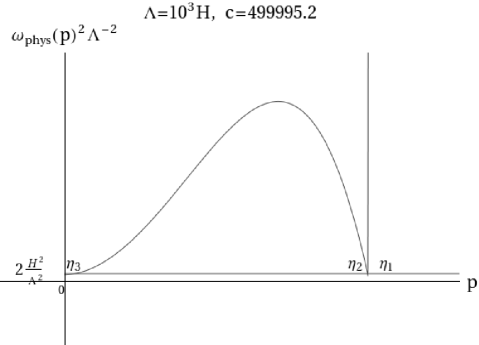
Figure 2: Modified dispersion relation used for the example in section A.2.

We now solve the equation (9) as done in section 3.1 and compute the main contribution to the bispectrum for the cubic coupling in (43), coming from the integration over the interval $[\eta_{\mbox{\text{{\tiny{\rm I}}}\text{{\tiny{\rm I}}}}},\eta_{\mbox{\text{{\tiny{\rm I}}}\text{{\tiny{\rm I}}}\text{{\tiny{\rm I}}}}}]$, as discussed in section 4.1.1. We neglect the other subdominant contributions. As expected, it is found that $\eta_{\mbox{\text{{\tiny{\rm I}}}\text{{\tiny{\rm I}}}}(\mbox{\text{{\tiny{\rm I}}}\text{{\tiny{\rm I}}}\text{{\tiny{\rm I}}}})}\simeq\eta_{{}_{2(3)}}$.

We compute the contribution to the bispectrum from the cubic interaction (43) using the formulas (57), (59) and (63) adapted to our case. We do not report their final expressions after being adapted, since the formulas are quite long and complicated but straightforward to be obtained. We find that in our example, the only enhanced configurations are close to the enfolded ones, where we have nearly critical points (see footnote 10). We plot the bispectrum rescaled by the standard slow-roll result and the modulus of $\beta_{\vec{k}}$ in figure 3 taking $\Lambda=10^{3}H$. The dispersion relation itself is plotted in figure 2.

For comparison, we also plot the correction to the bispectrum for cubic coupling obtained in [3] using the modified vacuum approach to transplanckian physics (from equation (3.17) in [3]). We observe that the shape of the modulations and the magnitude of enhancement are different between that case and the one of the modified dispersion relation given by equation (115).

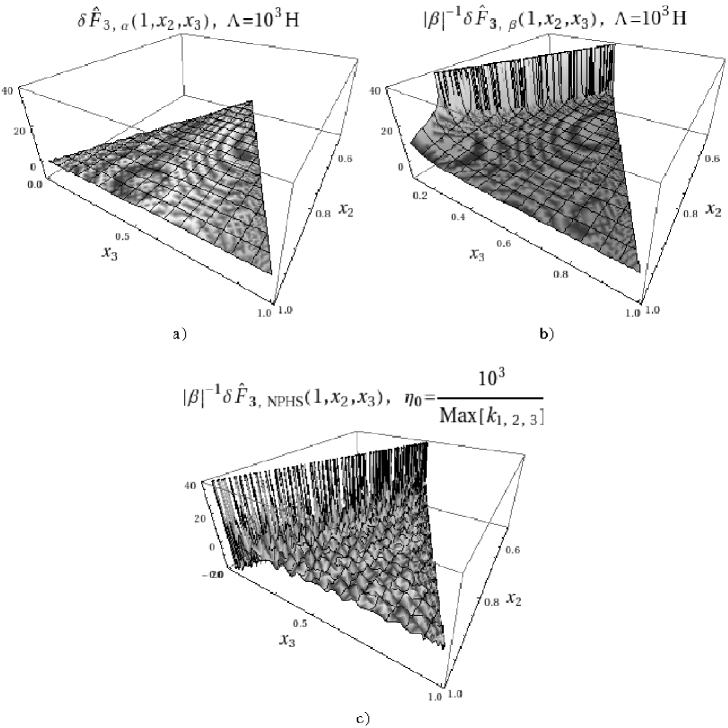
Figure 3: Cubic interactions $\sim\zeta^{{}^{\prime}3}$: a) Plot of the rescaled contribution to the bispectrum when all Green function are in the positive-frequency branch: negligible differences with the standard result (tiny superimposed oscillations). b) Plot of the rescaled contribution to the bispectrum when one of the Green functions is in the negative frequency branch: enhanced configurations for nearly critical points (see footnote 10). c) Plot of the rescaled contribution to the bispectrum when one of the Green function is in the negative frequency branch in the case of the modified vacuum modelling of transplanckian physics [3].

References

- [1] E. Komatsu et al., arXiv:0902.4759 [astro-ph.CO] J. M. Maldacena and G. L. Pimentel, arXiv:1104.2846 [hep-th]. I. Antoniadis, P. O. Mazur and E. Mottola, arXiv:1103.4164 [gr-qc].
- [2] J. M. Maldacena, JHEP 0305, 013 (2003) [arXiv:astro-ph/0210603].
- [3] R. Holman and A. J. Tolley, JCAP 0805, 001 (2008) [arXiv:0710.1302 [hep-th]].
- [4] P. D. Meerburg, J. P. van der Schaar and M. G. Jackson, JCAP 1002, 001 (2010) [arXiv:0910.4986 [hep-th]].
- [5] A. Kempf, Phys. Rev. D 63, 083514 (2001) [arXiv:astro-ph/0009209]. A. Kempf and J. C. Niemeyer, Phys. Rev. D 64, 103501 (2001) [arXiv:astro-ph/0103225]. S. F. Hassan and M. S. Sloth, Nucl. Phys. B 674 (2003) 434 [arXiv:hep-th/0204110]. R. Easther, B. R. Greene, W. H. Kinney and G. Shiu, Phys. Rev. D 66, 023518 (2002) [arXiv:hep-th/0204129]. R. Easther, B. R. Greene, W. H. Kinney and G. Shiu, Phys. Rev. D 64, 103502 (2001) [arXiv:hep-th/0104102].
- [6] K. Schalm, G. Shiu and J. P. van der Schaar, JHEP 0404 (2004) 076 [arXiv:hep-th/0401164]. K. Schalm, G. Shiu and J. P. van der Schaar, AIP Conf. Proc. 743 (2005) 362 [arXiv:hep-th/0412288].
- [7] U. H. Danielsson, Phys. Rev. D 66, 023511 (2002) [arXiv:hep-th/0203198]. U. H. Danielsson, JHEP 0207 (2002) 040 [arXiv:hep-th/0205227].
- [8] D. Seery and J. E. Lidsey, JCAP 0506 (2005) 003 [arXiv:astro-ph/0503692].
- [9] X. Chen, M. x. Huang, S. Kachru and G. Shiu, JCAP 0701 (2007) 002 [arXiv:hep-th/0605045].
- [10] J. Martin and R. H. Brandenberger, Phys. Rev. D 63, 123501 (2001) [arXiv:hep-th/0005209].
- [11] J. Martin and R. H. Brandenberger, Phys. Rev. D 65, 103514 (2002) [arXiv:hep-th/0201189]. J. Martin and R. Brandenberger, Phys. Rev. D 68 (2003) 063513 [arXiv:hep-th/0305161].
- [12] M. Lemoine, M. Lubo, J. Martin and J. P. Uzan, Phys. Rev. D 65 (2002) 023510 [arXiv:hep-th/0109128].
- [13] D. Mattingly, Living Rev. Rel. 8 (2005) 5 [arXiv:gr-qc/0502097]. T. Jacobson, S. Liberati and D. Mattingly, Annals Phys. 321 (2006) 150 [arXiv:astro-ph/0505267].
- [14] T. Jacobson and D. Mattingly, Phys. Rev. D 64 (2001) 024028 [arXiv:gr-qc/0007031].
- [15] D. Mattingly and T. Jacobson, arXiv:gr-qc/0112012.
- [16] M. V. Libanov and V. A. Rubakov, JCAP 0509 (2005) 005 [arXiv:astro-ph/0504249].
- [17] T. Jacobson, S. Liberati and D. Mattingly, Annals Phys. 321, 150 (2006) [arXiv:astro-ph/0505267].
- [18] P. Horava, Phys. Rev. D79, 084008 (2009). [arXiv:0901.3775 [hep-th]].
- [19] D. J. H. Chung and K. Freese, Phys. Rev. D 61 (2000) 023511 [arXiv:hep-ph/9906542]. D. J. H. Chung and K. Freese, Phys. Rev. D 62, 063513 (2000) [arXiv:hep-ph/9910235]. D. J. H. Chung, E. W. Kolb and A. Riotto, Phys. Rev. D 65, 083516 (2002) [arXiv:hep-ph/0008126]. C. Csaki, J. Erlich and C. Grojean, Nucl. Phys. B 604, 312 (2001) [arXiv:hep-th/0012143]. S. L. Dubovsky, JHEP 0201, 012 (2002) [arXiv:hep-th/0103205].
- [20] D. Baumann and D. Green, arXiv:1102.5343 [hep-th]. A. J. Tolley and M. Wyman, Phys. Rev. D 81 (2010) 043502 [arXiv:0910.1853 [hep-th]].
- [21] A. Ashoorioon, D. Chialva and U. Danielsson, arXiv:1104.2338 [hep-th]. To appear in JCAP.
- [22] S. Corley and T. Jacobson, Phys. Rev. D 54, 1568 (1996) [arXiv:hep-th/9601073]. S. Corley, Phys. Rev. D 57, 6280 (1998) [arXiv:hep-th/9710075].
- [23] C. M. Bender, S. A. Orszag, “Asymptotic Methods for Scientists and Engeneers”, McGraw Hill, 1978, (Springer 1999).
- [24] J. Martin and D. J. Schwarz, Phys. Rev. D 67 (2003) 083512 [arXiv:astro-ph/0210090].
- [25] D. Babich, P. Creminelli and M. Zaldarriaga, JCAP 0408, 009 (2004) [arXiv:astro-ph/0405356].
- [26] A. Erdélyi, “Asymptotic Expansions”, Dover (New York) 1956.
- [27] P. Creminelli, JCAP 0310 (2003) 003 [arXiv:astro-ph/0306122].
- [28] R. H. Brandenberger and J. Martin, Phys. Rev. D 71 (2005) 023504 [arXiv:hep-th/0410223].
- [29] B. R. Greene, K. Schalm, G. Shiu and J. P. van der Schaar, JCAP 0502 (2005) 001 [arXiv:hep-th/0411217].
- [30] U. H. Danielsson, Phys. Rev. D 71 (2005) 023516 [arXiv:hep-th/0411172].