Helicity-dependent photocurrents in graphene layers
excited by mid-infrared radiation of a CO₂-laser

Abstract

We report the study of the helicity driven photocurrents in graphene excited by mid-infrared light of a CO₂-laser. Illuminating an unbiased monolayer sheet of graphene with circularly polarized radiation generates – under oblique incidence – an electric current perpendicular to the plane of incidence, whose sign is reversed by switching the radiation helicity. We show that the current is caused by the interplay of the circular $ac$ Hall effect and the circular photogalvanic effect. Studying the frequency dependence of the current in graphene layers grown on the SiC substrate we observe that the current exhibits a resonance at frequencies matching the longitudinal optical phonon in SiC.

I Introduction

Recently graphene has attracted enormous attention because its unusual electronic properties make possible relativistic experiments in a solid state environment and may lead to a large variety of novel electronic devices p1 ; p2 ; p2bis ; p2bis2 . One of the most interesting physical aspects of graphene is that its low-energy excitations are massless, chiral Dirac fermions. The chirality of electrons in graphene leads to a peculiar modification of the quantum Hall effect p3 ; p4 , and plays a role in phase-coherent phenomena such as weak localization p5 ; p6 . Most of current research in this novel material are focused on the transport and optical phenomena. In our recent work, we reported on the observation of the circular $ac$ Hall effect (CacHE) prl2010 which brings the transport and optical properties of graphene together: In CacHE an electric current, whose sign is reversed by switching the radiation helicity, is caused by the crossed electric and magnetic fields of terahertz (THz) radiation. The photocurrent is proportional to the light wavevector and may, therefore, also be classified as photon drag effect prl2010 ; Ch7Barlow54 ; Ch7Danishevskii70p544 ; Ch7Gibson70p75 ; grinberg:class ; Ganichevbook ; condmat2010 . Classical theory of CacHE, well describing the experiment at THz frequencies, predicts that for $\omega\tau\gg 1$, with $\omega$ being the radiation angular frequency and $\tau$ momentum relaxation time of electrons, the $ac$ Hall effect is suppressed.

Here we demonstrate, however, that helicity driven photocurrents can be detected applying a mid-infrared CO₂ laser operating at much higher light frequencies where the condition $\omega\tau\gg 1$ is satisfied. Our results show that in this case, due to the fact that the classical CacHE is substantially diminished, much finer effects, such as circular photogalvanic effect (CPGE), well known for noncentrosymmetric bulk and low dimensional semiconductors Ganichevbook ; Ch7Asnin78p74 ; APL2000 ; PRB2003 ; IvchenkoGanichev , become measurable. We present a phenomenological and microscopic theory of photocurrents in graphene and show that the experimental proof of the interplay of CacHE and circular PGE of comparable strength comes from the spectral behavior of the photocurrent.

Our experiments demonstrate that variation of the radiation frequency may result in an inversion of the photocurrent sign. We show that the light frequency, at which the inversion takes place, changes from sample to sample. Tuning the radiation frequency in the operation range of a mid-infrared CO₂ laser we also observed a resonant-like behaviour of the photocurrent in graphene grown on the Si-terminated face of a 4H-SiC(0001) substrate: its amplitude drastically increases at frequency $f=29.2$ THz ($\lambda=$ 10.26 $\mu$m). The microscopic origin of the resonant photocurrent is unclear, but we show that its position is correlated with the high frequency edge of the reststrahlen band and, correspondingly, to the energy of the LO phonon in 4H-SiC. Besides the helicity driven electric currents we also present a detailed study of a photocurrents excited by unpolarized and linearly polarized light, also observed in our experiments, and discuss their origin.

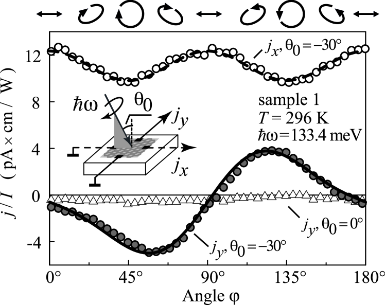
Figure 1: Photocurrent $j$ normalized by the light intensity $I$ as a function of the angle $\varphi$ defining radiation helicity. Here $j(\varphi)$ is measured at room temperature applying radiation with $\hbar\omega=133.4$ meV ($\lambda=9.27$ $\mu m$). Open and full circles show the longitudinal, $j_{x}$, and transverse, $j_{y}$, photocurrents measured at oblique incidence ($\theta_{0}=-30^{\circ}$) along and perpendicular to the light propagation, respectively. Triangles demonstrate that the photoresponce vanishes at normal incidence ($\theta_{0}=0^{\circ}$). Lines show fits according to Eqs. (1), (2) obtained using only photocurrent magnitudes as fitting parameters [see also Eqs. (3), (4) and (5), (6)]. The inset shows the experimental geometry, the plane of incidence of the radiation and the arrangement of contacts (black dots) at the edges of graphene. The ellipses on top illustrate the polarization states for various $\varphi$ for light incident on the sample as seen along the propagation direction.

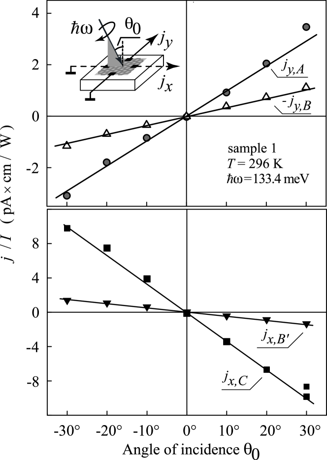
Figure 2: Angle of incidence dependence of the various photocurrent contributions detected in the transverse (upper panel) and longitudinal (lower panel) geometries. Here $j_{y,A}(\theta_{0})$, $j_{y,B}(\theta_{0})$, $j_{x,B^{\prime}}(\theta_{0})$, and $j_{x,C}(\theta_{0})$ are obtained by measuring the helicity dependence of the photocurrent and fitting it by the Eqs. (1) and (2) [see also Eqs. (3), (4) and (5), (6)]. The solid lines are fits after $j\propto\theta_{0}$. The inset shows the experiment geometry.

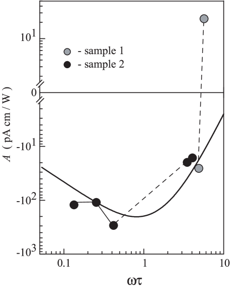
Figure 3: Helicity driven photocurrents given by the coefficient $A=j_{y,A}/(I\theta_{0})$ as function of $\omega\tau$. Solid curves show calculations of the $ac$ Hall effect. The results of calculations and the low frequency data ($\omega\tau<0.4$) are given after prl2010 , see also Eqs. (7).

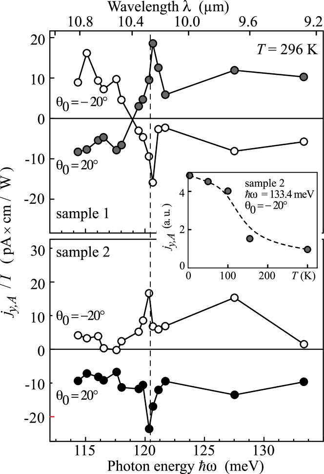
Figure 4: Spectral dependence of $j_{y,A}$ obtained for circularly polarized light ($\varphi=45^{\circ}$) and two angles of incidence $\theta_{0}=\pm 30^{\circ}$. Upper and lower panels show the data for samples 1 and 2, respectively. The inset shows the temperature dependence of $j_{y,A}$ measured in sample 2.

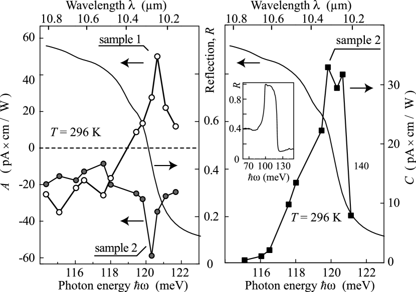
Figure 5: Spectral behaviour of $A=j_{y,A}/(I\theta_{0})$ (left panel) and $C=j_{x,C}/(I\theta_{0})$ (right panel) in the vicinity of resonance. Solid curves show the reflection of the sample. We note that measurements of the reflection from the graphene and the back side of the sample yield the almost the same result. The inset shows the reflection spectrum in a larger frequency range.

II Experiment

The experiments were carried out on large area graphene monolayers prepared by high temperature Si sublimation of semi-insulating silicon carbide (SiC) substrates LaraAvival09 . The samples have been grown on the Si-terminated face of a 4H-SiC(0001) substrate. The reaction kinetics on the Si-face is slower than on the C-face because of the higher surface energy, which helps homogeneous and well controlled graphene formation Emtsev09 . Graphene was grown at 2000^∘C and 1 atm Ar gas pressure resulting in monolayers of graphene atomically uniform over more than 1000 $\mu$m², as shown by low-energy electron microscopy Virojanadara08 . Four contacts have been centered along opposite edges of $5\times 5$ mm² square shaped samples by deposition of 3 nm of Ti and 100 nm of Au (see inset in Fig. 1). The measured resistance was about 2 k$\Omega$. From low-field Hall measurements, the manufactured material is $n$-doped due to the charge transfer from SiC Emtsev09 ; Bostwick09 . We used two layers of non-conductive polymers la11 to protect graphene samples from the undesired doping in the ambient atmosphere and to control carrier concentration in the range ($3$ to $7$)$\times$10¹² cm^-2, mobility is of the order of 1000 cm²/Vs and the Fermi energies $E_{F}\sim 300$ meV. All parameters are given for room temperature.

To generate photocurrents we applied mid-infrared radiation of tunable CO₂-lasers with operating spectral range from 9.2 to 10.8 $\mu$m (32.6 THz$\leq f\leq 27.8$ THz) corresponding to photon energies ranging from 114 to 135 meV Ganichevbook . For these wavelengths the conditions $\hbar\omega<E_{F}$ and $\omega\tau\gg 1$ hold. Two laser systems were used; a medium power $Q$-switched laser with the pulse duration of 250 ns (repetition frequency of 160 Hz) and low power continuous-wave ($cw$) laser modulated at $120$ Hz. The samples were illuminated at oblique incidence with peak power, $P$, of about 500 W and about 0.1 W for Q-switched and $cw$ laser, respectively. The radiation power was controlled by photon drag detector Ganichev84p20 and/or MCT detector. The radiation was focused in a spot of 1 mm diameter being much smaller than the sample size even at oblique incidence exfoliated . The initial laser radiation polarization vector was oriented along the $x$-axis. Applying Fresnel $\lambda/4$ rhomb we modified the laser light polarization from linear to elliptical. The helicity $P_{circ}$ of the light at the Fresnel rhomb output was varied from -1 (left handed circular, $\sigma_{-}$) to +1 (right handed circular, $\sigma_{+}$) according to $P_{circ}=\sin 2\varphi$, where $\varphi$ is the azimuth of Fresnel s romb. Angle $\varphi=0$ corresponds to the position of the Fresnel rhomb when its symmetry plane is oriented perpendicular to the $y$-axis. The polarization ellipses for some angles $\varphi$ are shown on top of Fig. 1.

The geometry of the experiment is sketched in the inset in Fig. 1. The incidence angle $\theta_{0}$ was varied between $-30^{\circ}$ and +30^∘. In our experiments we used both transverse and longitudinal arrangements in which photoresponse was probed in directions perpendicular and parallel to the light incidence plane, respectively (see insets in Fig. 1 and 2). The photosignal is measured and recorded with lock-in technique or with storage oscilloscope. The experiments were carried in the temperature range from 4.2 K to 300 K.

The signal in unbiased samples is observed under oblique incidence for both transversal and longitudinal geometries, where the current is measured in the direction perpendicular and parallel to the plane of incidence, respectively. Figure 1 shows the photocurrent as a function of the angle $\varphi$ for these geometries. The current behaviour upon variation of radiation ellipticity is different when measured normal and along to the light incidence plane.

The photocurrent for the transversal geometry, $j_{y}$, (see full circles in Fig. 1) is dominated by the contribution proportional to the photon helicity $P_{circ}=\sin 2\varphi$; it reverses when the light polarization switches from the left-handed ($\varphi=45^{\circ}$) to the right-handed ($\varphi=135^{\circ}$) light. The overall dependence of $j_{y}$ on $\varphi$ is more complex and well described by

$$j_{y}=j_{y,A}\sin 2\varphi+j_{y,B}\sin 4\varphi+\xi\>,$$ (1)

where $j_{y,A}=AI\theta_{0}$ and $j_{y,B}=BI\theta_{0}$ are the magnitudes of the circular and linear contributions, respectively. Here $I$ is the light intensity. It is noteworthy that the offset $\xi$ is detected only in some measurements; It is almost zero and is neglected in the analysis below. The fit to the above equation is shown in Fig. 1 by solid line. We emphasize, that exactly the same functional behaviour is obtained from a phenomenological picture and microscopic models outlined below. Note that for circularly polarized light, the current is solely determined by the first term in Eq. (1), because the degree of linear polarization is zero and, in this case, the second term vanishes. Our experiments show that $j_{y,A}$ and $j_{y,B}$ are odd functions of the incidence angle $\theta_{0}$; a variation of $\theta_{0}$ in the plane of incidence changes the sign of the currents, which vanish for normal incidence, $\theta_{0}$=0 (see triangles in Fig. 1). This behaviour is illustrated by Fig. 2 showing the angle of incidence dependence of the photocurrents $j_{A}$, $j_{B}$ and $j_{C}$ determining the magnitudes of the circular photocurrent and that depending on the degree of linear polarization, respectively.

In the longitudinal geometry (open circles in Fig. 1), the current sign and magnitude are the same for left-handed to right-handed circular polarized light and its overall dependence on $\varphi$ can be well fitted by

$$j_{x}=j_{x,B^{\prime}}\cos 4\varphi+j_{x,C},$$ (2)

where $j_{x,B^{\prime}}=B^{\prime}I\theta_{0}$ and $j_{x,C}=CI\theta_{0}$ are the magnitudes of the linear and polarization-independent contributions, respectively. The fit after this equation is shown in Fig. 1 by dashed line. Like in transversal geometry the photocurrent angular dependence is in agreement with the theory discussed below.

Figure 3 shows spectral behaviour of the circular photocurrent given by the coefficient $A=j_{y,A}/I\theta_{0}$. In this figure $A$ is plotted as a function of $\omega\tau$ for both graphene samples. Besides the data obtained for light with the photon energy exceeding 110 meV we included here the results obtained in the same samples but at much lower THz frequencies $f\lesssim 4$ THz with $\hbar\omega\lesssim 16$ meV. The latter data as well as the calculated dependences of the $ac$ Hall effect are taken from our previous work prl2010 . It is seen that in the second sample the theory of the $ac$ Hall effect describes well the experiment in the whole frequency range, including the high frequency data. While the sign and the magnitude of the current in the first sample measured at low frequency edge of the CO₂-laser operation also fits well to the smooth curve of the $ac$ Hall effect (see open circles in Fig. 3) at high frequencies we observed that the signal abruptly changes its sign with rising frequency. The observed spectral inversion of the photocurrent’s sign reveals that only $ac$ Hall effect can not describe the experiment.

Figure 4 shows the results of the more detailed study of the circular photocurrent’s frequency dependence. The data were obtained by using the whole accessible, but very narrow, operating range of the CO₂-laser (114 meV $<\hbar\omega<135$ meV). Full and open circles in this figure correspond to the data obtained for two opposite angles of incidence $\theta_{0}=\pm 20^{\circ}$. It is seen that the detected in sample 1 reversal of the current direction takes place at $\hbar\omega_{inv}\simeq 119$ meV. Here, $\omega_{inv}$ indicates the frequency of the sign inversion. The drastic difference in the photocurrent’s spectral behaviour detected for samples with almost the same mobility and carrier density but prepared not in the same growth circle we attribute to the change of coupling between graphene layer and the substrate. In fact, this parameter is crucial for the mechanisms of the photocurrent generation. It may be different from sample to sample and it is difficult to control.

Besides the spectral inversion, we observe another remarkable feature of the photocurrent: in both samples we detected a resonance increase of the current magnitude at $\hbar\omega\simeq 121$ meV (see Fig. 4 and left panel in Fig. 5). Similar resonance-like behaviour is detected for the polarization-independent longitudinal photocurrent (see right panel in Fig. 5). The position of the resonance corresponds to the longitudinal optical (LO) phonon energy in 4H-SiC. In order to prove this we measured the sample reflection for the graphene and the substrate sides. The results for both sides almost coincide with each other: the reflection shows the reststrahlen band behaviour (see the inset in Fig. 5). Solid curves in the left and right panels in Fig. 5 show that the high frequency edge of the reststrahlen band, which corresponds to the LO phonon energy in 4H-SiC, coincide with the resonance position. The detailed study of the resonance photocurrent and its power dependence is beyond the scope of the present work.

To summarize the experimental part we demonstrate that illumination of graphene monolayers by mid-infrared radiation at oblique incidence results in the generation of photocurrents. Their directions and magnitudes are determined by the polarization of the radiation. At the frequencies about $f=29.2$ THz ($\hbar\omega=121$ meV) we observed resonance feature and sign inversion of the photocurrent. The latter property is sample dependent.

III Theory

Below we present phenomenological analysis of the photocurrents in graphene as well as their microscopic models. We demonstrate that the experimentally observed incidence angle, linear polarization and helicity dependences of the photocurrents correspond to phenomenological models. The magnitudes of the photocurrents and their polarization dependencies are also in good agreement with theoretical predictions.

III.1 Phenomenological analysis

The ideal honeycomb lattice of graphene is described by the point group $D_{6\rm h}$ containing the spatial inversion. As a result, photocurrent generation is possible provided that the joint action of electric, $\bm{E}$, and magnetic, $\bm{B}$, fields of the radiation is taken into account or provided that the allowance for the radiation wave vector, $\bm{q}$, transfer to electron ensemble is made. In the former case the Cartesian components of the current are proportional to the bi-linear combinations $E_{\alpha}B_{\beta}^{*}$, while in the latter case to the combinations $q_{\alpha}E_{\beta}E_{\gamma}^{*}$. Here Greek subscripts enumerate Cartesian components. For the plane wave its wave vector, electric and magnetic fields are interrelated, therefore, for the purposes of the phenomenological analysis it is enough to express the photocurrent density via the combinations $q_{\alpha}E_{\beta}E_{\gamma}^{*}$ as condmat2010

$$j_{x}/I=T_{1}q_{x}\frac{|e_{x}|^{2}+|e_{y}|^{2}}{2}+T_{2}q_{x}\frac{|e_{x}|^{2}-|e_{y}|^{2}}{2},$$ (3a)

$$j_{y}/I=T_{2}q_{x}\frac{e_{x}e_{y}^{*}+e_{x}^{*}e_{y}}{2}-\tilde{T}_{1}q_{x}P_{\rm circ}\hat{e}_{z}.$$ (3b)

where $x$ and $y$ are the axes in the graphene plane, and $z$ is the structure normal, the radiation is assumed to be incident in $(xz)$ plane, $\hat{\bm{e}}$ is the unit vector in light propagation direction and $\bm{e}$ is the (complex) polarization vector of radiation, $P_{\rm circ}$ is the circular polarization degree and $\bm{q}$ is the radiation wave vector. Additional contributions to the photocurrents, involving $z$ component of electric field are analyzed in Ref. condmat2010 . These effects are expected to be strongly suppressed in ideal samples and for moderate radiation frequencies. Expressions (3) can be rewritten via incidence angle, $\theta_{0}$, and angle $\varphi$ determining the radiation helicity as Eqs. (1), (2). It allows one to establish a link between phenomenological constants $T_{1}$, $T_{2}$ and $\tilde{T}_{1}$ and fitting parameters $A$, $B$ and $C$ used to describe the experimental data, see Figs. 1 and 2. Namely, at small incidence angles

$$A\propto\tilde{T}_{1},\quad B\propto T_{2},\quad\mbox{and}\quad C\propto T_{1}.$$ (4)

It follows from Eqs. (3) that photocurrent contains, in general, three contributions illustrated in Fig. 6, panels (a)–(c). First one, schematically illustrated in Fig. 6(a) results in the polarization-independent photocurrent flowing along the light incidence plane.

In accordance with the general line of the paper we pay special attention to the photocurrent contribution presented in Fig. 6(b) where the generation of the transversal to the light incidence plane current is shown. This current component is dependent on the radiation helicity: by changing photon from right- to left- circularly polarized, current changes its direction. This is nothing but the CacHE uncovered recently in graphene Ref. prl2010 . In addition, transversal photoresponse contains a component, being sensitive to the linear polarization of radiation, see Fig. 6(c).

The photocurrent components described by Eqs. (3) can also be qualified as photon drag effects Ganichevbook ; ivchenkobook since in their phenomenological description the photon wave vector is involved. The direction of the photocurrent changes its sign upon reversal of the incidence angle. The contributions given by Eq. (3a) and the first term in the Eq. (3b) can be easily understood as transfer of linear momenta of photons to the electron system JETP1982 and is recently discussed for graphene condmat2010 ; Entin:gr . The circular photon drag current described by the second term on the right hand side of Eq. (3b) is due to transfer of both linear and angular momenta of photons to free carriers. The circular photon drag effect was discussed phenomenologically Ivchenko1980 ; Belinicher1981 and observed in GaAs quantum wells in the mid-infrared range Shalygin2006 and in metallic photonic crystal slabs Hatano09 . We note, that while the microscopic description of the circular photocurrent in graphene in terms of $ac$ Hall effect is relevant to the relatively low radiation frequencies range at high frequencies all photocurrent contributions can be conveniently treated in terms of photon drag effect.

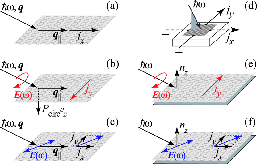
Figure 6: Schematic illustration of the possible contributions to the photon drag and photogalvanic effects. Panels (a)-(c): polarization independent, circular and linear photon drag effects, Eqs. (3). Panel (d) shows the experimental geometry. Panels (e)-(f): photogalvanic effects allowed by symmetry in graphene samples deposited on substrates.

The real structures, however, are deposited on a substrate, which removes the equivalence of the $z$ and $-z$ directions and reduces the symmetry to the $C_{6\rm v}$ point group. Such symmetry reduction makes photogalvanic effects possible. The photogalvanic effects give rise to the linear and circular photocurrents condmat2010 :

$$j_{x}/I=\chi_{l}\frac{e_{x}e_{z}^{*}+e_{x}^{*}e_{z}}{2}\>,$$ (5a)

$$j_{y}/I=\chi_{l}\frac{e_{y}e_{z}^{*}+e_{y}^{*}e_{z}}{2}+\chi_{c}P_{\rm circ}\hat{e}_{x}\>,$$ (5b)

described by two independent parameters $\chi_{l}$ and $\chi_{c}$. Schematically, these contributions to the photocurrent are shown in Fig. 6(e), (f). It follows from Eqs. (5) that the linear photocurrent flows along the projection of the electric field onto the sample plane and it has both $x$ and $y$ components, in general. By contrast, circular photocurrent flows transverse to the radiation incidence plane, i.e. along $y$ axis in the chosen geometry. Despite the fact that the photogalvanic effects described by Eqs. (5) require the out-of-plane component of the incident radiation, they may be important for real graphene samples as it follows from the microscopic model, see Sec. III.2.

Equations (5) reveal that transverse and longitudinal photogalvanic currents vary upon change of the radiation polarization similarly to the $ac$ Hall (photon-drag) photocurrents given by Eqs. (3).

Thus, photogalvanic effects described by Eqs. (5) make only additional contributions to the constants $A$, $B$ and $C$ in phenomenological expressions (1), (2). In the case that the photocurrent is driven solely by photogalvanic effects these constants are given by,

$$A\propto\chi_{c},\quad\mbox{and}\quad-2B=C\propto\chi_{l}.$$ (6)

It follows from Eqs. (3) and (5) that the phenomenological theory, which is based solely on symmetry arguments and does not require knowledge of the microscopic processes of light-matter coupling in graphene, describes well the polarization dependences of the photocurrents presented in Fig. 1 and fitted by Eqs. (1) and (2). The incidence angle dependences presented in Fig. (2) are also in line with phenomenological description.

Hence, the phenomenological analysis is presented, which yields a good agreement with the experiment. Schematical illustration Fig. 6 as well as Eqs. (3) and (5) show that both the $ac$ Hall effect and photogalvanic effect have almost the same polarization and incidence angle dependences. Therefore, the analysis of polarization and incidence angle dependencies of the photocurrents is not enough to establish their microscopic origins. Therefore, extra arguments based on microscopic model are needed.

III.2 Microscopic mechanisms

Before turning to the presentation of the microscopic models, let us introduce the different regimes of radiation interaction with electron ensemble in graphene depending on the photon frequency, $\omega$, electron characteristic energy (Fermi energy), $E_{F}$, and its momentum relaxation rate $1/\tau$. We assume that the condition $E_{F}\tau/\hbar\gg 1$ is fulfilled (which is the case for the samples under study) making possible to treat electrons in graphene as free.

If photon energy is much smaller compared with electron Fermi energy, $\hbar\omega\ll E_{F}$, the classical regime is realized. In this case the electron motion can be described within the kinetic equation for the time $t$, momentum $\bm{p}$ and position $\bm{r}$ dependent distribution function $f(\bm{p},\bm{r},t)$.

An increase of the photon energy makes classical approach invalid. If $\hbar\omega\leqslant 2E_{F}$ the direct interband transitions are not possible and the radiation absorption as well as the photocurrent generation are possible via indirect (Drude-like) transitions. It is worth to mention that if $\hbar/\tau\ll\hbar\omega\leqslant E_{F}$ the transitions are intraband, while for $E_{F}<\hbar\omega\leqslant 2E_{F}$ the initial state for the optical transition may be in the valence band.

In what follows we restrict ourselves to the indirect intraband transitions, assuming that $\hbar/\tau\ll\hbar\omega\leqslant E_{F}$ which corresponds to our experiments with CO₂ laser excitation. The results for the classical frequency range, $\hbar\omega\ll E_{F}$, relevant for THz excitation, will be also briefly discussed.

III.2.1 High frequency (ac) Hall effect

The microscopic calculation of the ac Hall effect in the classical frequency range, where $\hbar\omega\ll E_{F}$ was carried out in Refs. prl2010 ; condmat2010 . Thus, we give here only the final result of this work obtained within the framework of the Boltzmann equation with allowance for both $\bm{E}\bm{B}$ (ac Hall effect) and $qE^{2}$ (spatial dispersion effect) contributions. The circular photocurrent is given for degenerate electrons by

$$j_{A}=A\theta_{0}\sin{2\varphi}=\\ =q\theta_{0}\frac{e^{3}{\tau_{1}(v\tau_{1}E)^{2}}}{{2\pi\hbar^{2}(1+\omega^{2}\tau_{1}^{2})}}P_{\rm circ}\left(1+\frac{\tau_{2}}{\tau_{1}}\right)\frac{1-r}{1+\omega^{2}\tau_{2}^{2}},$$ (7)

Here $q=\omega/c$, we have replaced for the small incidence angles $q\sin{\theta_{0}}\approx q\theta_{0}$, $v$ is the electron velocity in graphene, $\tau_{1}$ and $\tau_{2}$ are the relaxation times of first and second angular harmonics of the distribution function describing the decay of the electron momentum and momentum alignment prl2010 ; condmat2010 ; perel73 , and $r=d{\rm ln}\tau_{1}/d{\rm ln}\varepsilon$ ($\varepsilon$ is the electron energy). The frequency dependence is presented by a solid curve in Fig. 3. At low frequencies $\omega\tau\ll 1$ the parameter $A$ and, correspondingly, the circular photocurrent raises with the frequency increase as $\omega\tau$. In the high frequency regime $\omega\tau\gg 1$, by contrast, the circular photocurrent related with CacHE drops as

$$j_{A}\propto\frac{1}{\omega^{3}\tau},\quad\frac{\hbar}{\tau}\ll\hbar\omega\ll E_{F}.$$ (8)

Calculations show that for our $n$-type structures the constant $A$ describing CacHE photocurrent is negative in the wholef frequency range, achieves its maximum absolute value for $\omega\tau\sim 1$ and describes well the experiment at least at low frequencies (see Figure 3).

The solution of the Boltzmann equation also yields linear photocurrents in longitudinal ($j_{B^{\prime}}$ and $j_{C}$) and transverse ($j_{B}$) geometries prl2010 ; condmat2010 . These photocurrents are proportional to the constants $T_{1}$ and $T_{2}$ in Eqs. (3). They describe well polarization dependences presented in Fig. 1 providing the polarization independent longitudinal photocurrent as well as photocurrent contributions varying with the change of degree of linear polarization as $\sin 4\varphi$ and $\cos 4\varphi$. These constants $T_{1}$ and $T_{2}$ as functions of frequency diverge as $1/\omega$ at $\omega\tau\to 0$ and decay as $1/\omega^{3}$ for $\omega\tau\gg 1$. As a result,

$$j_{B},j_{C}\propto\frac{1}{\omega^{2}},\quad\frac{\hbar}{\tau}\ll\hbar\omega\ll E_{F}.$$ (9)

It should be noted that the longitudinal linear photocurrent can change its direction as function of the radiation frequency depending on the dominant scattering mechanism condmat2010 .

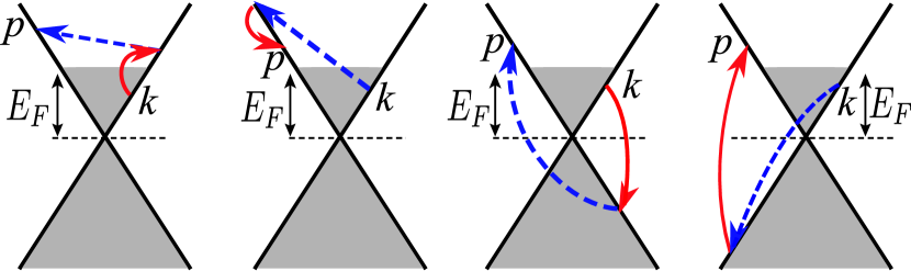
Figure 7: Schematic illustration of the processes responsible for the drag effect in the quantum frequency range under intraband transitions ($\hbar\omega\leqslant E_{F}$). Solid/red arrows denote electron-photon interaction, dashed/blue arrows denote electron scattering caused by impurities or phonons. Filled/gray area shows the part of energy spectrum filled with electrons.

To present a complete picture of the photocurrent formation due to Drude absorption we turn to the quantum frequency range and assume that $\hbar\omega\leqslant E_{F}$, while $\omega\tau\gg 1$. The absorption of the electromagnetic wave in the case of intraband transitions should be accompanied with the electron scattering, otherwise energy and momentum conservation laws can not be satisfied. The matrix elements describing electron transition from $\bm{k}$ to $\bm{p}$ state with the absorption ($M_{\bm{p},\bm{k}}^{{\rm abs},\bm{q}}$) and emission ($M_{\bm{p},\bm{k}}^{{\rm emit},\bm{q}}$) of a photon with the wave vector $\bm{q}$ are calculated in the second order of perturbation theory as

$$M_{\bm{p},\bm{k}}^{{\rm abs},\bm{q}}=\sum_{\nu=\pm}\left\{\frac{V^{+\nu}_{\bm{p},\bm{k}+\bm{q}}R^{\nu+}_{\bm{k}+\bm{q},\bm{k}}}{\varepsilon_{\bm{k}}^{+}-\varepsilon_{\bm{k}+\bm{q}}^{\nu}+\hbar\omega}+\frac{R^{+\nu}_{\bm{p},\bm{p}-\bm{q}}V^{\nu+}_{\bm{p}-\bm{q},\bm{k}}}{\varepsilon_{\bm{k}}^{+}-\varepsilon_{\bm{p}-\bm{q}}^{\nu}}\right\},\\$$ (10a)

$$M_{\bm{p},\bm{k}}^{{\rm emit},\bm{q}}=\sum_{\nu=\pm}\left\{\frac{V^{+\nu}_{\bm{p},\bm{k}-\bm{q}}R^{\nu+}_{\bm{k}-\bm{q},\bm{k}}}{\varepsilon_{\bm{k}}^{+}-\varepsilon_{\bm{k}-\bm{q}}^{\nu}-\hbar\omega}+\frac{R^{+\nu}_{\bm{p},\bm{p}+\bm{q}}V^{\nu+}_{\bm{p}+\bm{q},\bm{k}}}{\varepsilon_{\bm{k}}^{+}-\varepsilon_{\bm{p}+\bm{q}}^{\nu}}\right\}.$$ (10b)

Here superscript $\nu$ enumerates conduction band ($\nu=+$) and valence band ($\nu=-$), respectively, $R_{\bm{k}\pm\bm{q},\bm{k}}^{\nu\nu^{\prime}}$ is the electron-photon interaction matrix element, $V_{\bm{p},\bm{k}}^{\nu\nu^{\prime}}$ is the matrix element describing electron scattering by an impurity or a phonon. We note that the incident electromagnetic wave is assumed to be classical, hence the electron-photon interaction matrix elements are the same for the emission and absorption processes, $M_{\bm{p},\bm{k}}^{{\rm emit},\bm{q}}=M_{\bm{k},\bm{p}}^{{\rm abs},\bm{q}}\equiv M_{\bm{p},\bm{k}}^{\bm{q}}$ because the number of photons in this wave is large. It was assumed also that the graphene is $n$ doped so the initial and final states lie in the conduction band. The intermediate state, however, can be in conduction or in valence bands, see Fig. 7.

The dc current density can be calculated as grinberg:quant

$$\bm{j}=e\frac{8\pi}{\hbar}\sum_{\bm{k},\bm{p}}[\bm{v}_{\bm{p}}\tau_{1}(\varepsilon_{p})-\bm{v}_{\bm{k}}\tau_{1}(\varepsilon_{k})]|M_{\bm{p},\bm{k}}^{\bm{q}}|^{2}\\ [f(\varepsilon_{k})-f(\varepsilon_{p})]\delta(\varepsilon_{p}-\varepsilon_{k}-\hbar\omega),$$ (11)

where $\bm{v}_{\bm{k}}$ is the electron velocity in the state with the wave vector $\bm{k}$, $\tau_{1}(\varepsilon_{k})$ is the momentum relaxation time, $f(\varepsilon_{k})$ is the Fermi-Dirac distribution function, $\varepsilon_{k}=\hbar vk$ is the electron dispersion in graphene.

Let us assume that the electron scattering is provided by the short-range impurities acting within given valley, intervalley scattering processes are disregarded. The matrix elements for the impurity scattering are given by

$$V^{++}_{\bm{p}\bm{k}}=\frac{V_{0}}{2}\left[1+e^{\mathrm{i}(\varphi_{\bm{k}}-\varphi_{\bm{p}})}\right],\quad V^{-+}_{\bm{p}\bm{k}}=\frac{V_{0}}{2}\left[1-e^{\mathrm{i}(\varphi_{\bm{k}}-\varphi_{\bm{p}})}\right],$$

$$V^{+-}_{\bm{p}\bm{k}}=\frac{V_{0}}{2}\left[1-e^{\mathrm{i}(\varphi_{\bm{k}}-\varphi_{\bm{p}})}\right],$$ (12)

where $V_{0}$ is real constant. As a result, one can express the coefficients $T_{1}$ and $T_{2}$ describing linear photocurrent in the following form ($\omega\tau\gg 1$)

$$T_{1}=-e^{3}v^{4}\frac{64\pi}{c\hbar\omega^{4}}\sum_{\bm{k}}[f(\varepsilon_{k})-f(\varepsilon_{p})]\frac{\varepsilon_{p}}{(\varepsilon_{k}+\varepsilon_{p})^{2}},$$ (13a)

$$T_{2}=-e^{3}v^{4}\frac{16\pi}{c\hbar\omega^{4}}\sum_{\bm{k}}[f(\varepsilon_{k})-f(\varepsilon_{p})]\frac{\varepsilon_{p}^{2}+\varepsilon_{k}^{2}+(\hbar\omega)^{2}}{\varepsilon_{k}(\varepsilon_{k}+\varepsilon_{p})^{2}}.$$ (13b)

Here $\varepsilon_{p}=\varepsilon_{k}+\hbar\omega$. It is noteworthy that Eqs. (13) are valid provided $\hbar\omega<E_{F}$. We note that although the scattering rates are not explicitly present in Eqs. (13), the scattering processes are crucial for the photocurrent formation.

If the photon frequency becomes much smaller as compared with the electron energies, $\hbar\omega\ll\varepsilon_{k},\varepsilon_{p}$, but $\omega\tau_{1},\omega\tau_{2}\gg 1$ the photon drag effect can be described classically. One can check that, in agreement with Eqs. (9), Eqs. (13) yield

$$T_{1}=2T_{2}=\frac{16\pi e^{3}v^{4}}{c\omega^{3}}\sum_{\bm{k}}\frac{f^{\prime}}{\varepsilon_{k}},$$ (14)

where $f^{\prime}=df/d\varepsilon$. In this frequency range values of $T_{1}$ and $T_{2}$ are identical to those presented in condmat2010 . Hence, linear photocurrents $j_{B},j_{C}\propto 1/\omega^{2}$ in this frequency range, see Eq. (9). Moreover, it can be shown that the circular high frequency Hall effect requires an allowance for the extra scattering and $\tilde{T}_{1}\propto 1/\omega^{4}$ making $j_{A}\propto 1/\omega^{3}$ in agreement with Eq. (8). Therefore, the frequency dependence of the circular photocurrent, $j_{A}$, is non-monotonous with the maximum at $\omega\tau\sim 1$. This is exactly the behavior observed experimentally, see Fig. 3, where the coefficient $A$ is plotted. Its absolute value first increases with the frequency and afterwards rapidly decreases. Overall agreement of the experimental data in sample 2 (shown by the points) and theoretical calculation (solid line) shown in Fig. 3 is good. The theory, however, does not describe the abrupt frequency dependence and change of the photocurrent’s sign observed in sample 1 (see gray circles in Fig. 3). In order to understand this behaviour we analyze the possible contributions of photogalvanic effects.

III.2.2 Microscopic mechanisms of photogalvanic effects

Real graphene samples are deposited on substrates. As we already noted above, it results in a lack of an inversion center and, correspondingly, allows for the photogalvanic effects. Phenomenological analysis demonstrated that the polarization and incidence angle dependences of the photogalvanic current are almost the same as for the ac Hall effect. It follows from the general arguments and phenomenological considerations summarized in Eqs. (5), that the photocurrent can be generated only with allowance for $z$-component of the incident electric field. However, for strictly two-dimensional model where only $\pi$-orbitals of carbon atoms are taken into account, no response at $E_{z}$ is possible. Therefore, microscopic mechanisms of the photogalvanic effects in graphene involve other bands in electron energy spectrum formed from the $\sigma$-orbitals of carbon atoms.

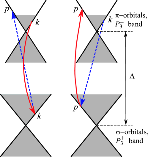
Figure 8: Schematic illustration of indirect intraband transitions with intermediate states in $P_{3}^{+}$ band which interfere with Drude transitions (shown in Fig. 7) and give rise to the photogalvanic effect. Solid red arrows are electron-photon interaction, dashed blue arrows are the electron scattering.

There are 6 irreducible representations $P_{1}^{+}$, $P_{1}^{-}$, $P_{2}^{+}$, $P_{2}^{-}$, $P_{3}^{+}$, and $P_{3}^{-}$ at $K$ (or $K^{\prime}$) point of the graphene’s Brillouin zone. The conduction and valence band states transform according to the $P_{3}^{-}$ representation: there are two basis functions $p_{z}^{(1)}$, $p_{z}^{(2)}$ being odd at the reflection in the graphene plane $z=0$. Symmetry analysis Bassani_old ; Bassani shows that the transitions in $z$ polarization are possible between these states (transforming according to $P_{3}^{-}$) and the states transforming according to $P_{3}^{+}$. The latter representation is described by two functions $s^{(1)}$ and $s^{(2)}$ which do not change their signs at the mirror reflection $z\to-z$. Under the symmetry operations which do not involve $z\to-z$ these wave functions transform like $p_{z}^{(1)}$, $p_{z}^{(2)}$. Representation $P_{3}^{+}$ corresponds to $\sigma$ orbitals of carbon atoms which form remote valence and conduction bands of graphene. Microscopic calculations performed within the basis of $2s$ and $2p$ atomic orbitals Bassani_old ; Bassani ; Zunger show that the distance from the $P_{3}^{-}$ states forming conduction and valence bands and closest deep valence bands $P_{3}^{+}$, $\Delta$, is about $10$ eV. It is remarkable, that the electron dispersion in these bands has the form, similar to that of conduction and valence bands: i.e. energy spectrum near $K$ (or $K^{\prime}$) point is linear, however, with different velocity, as it is schematically illustrated in Fig. 8.

Microscopically, circular photogalvanic effect arises due to the quantum interference of the Drude transitions represented in Fig. 7 (for $\bm{q}=0$) and the indirect intraband transitions with intermediate states in $P_{3}^{+}$ bands depicted in Fig. 8, similarly to the orbital mechanisms of the photogalvanic effects in conventional semiconductor nanostructures Tarasenko2007 ; PhysRevB.79.121302 ; tarasenko11 . Indeed, matrix elements of Drude transitions are proportional to the in-plane components of electric field $\bm{E}_{\parallel}$ and electron in-plane wave vectors in the initial $\bm{k}$, and final $\bm{p}$ states. The matrix elements of the indirect transitions via $P_{3}^{+}$ band are proportional to $E_{z}$ and do not contain linear in $\bm{k}$, $\bm{p}$ contributions. As a result, the interference contribution to the transition rate is proportional to both $\bm{E}_{\parallel}$ and $E_{z}$ and to the in-plane wave vector components giving rise to dc current. The presence of the substrate allows electron scattering between the states transforming according to $P_{3}^{+}$ and $P_{3}^{-}$ representations: for instance, the impurities located near the substrate surface or the phonons, propagating in the substrate, or the impurities adsorbed from the air to the graphene create an effective potential which is not symmetric with respect to $z\to-z$ mirror reflection. Hence, the interference contribution to the transition rate is non-vanishing.

Let us denote $\sigma$ orbital states transforming according to $P_{3}^{+}$ orbitals as $+^{\prime}$ and $-^{\prime}$ (we recall that the superscripts $+$ and $-$ denote the conduction and valence band states in Eq. (10), respectively). We assume that the relevant interband optical matrix element has a form note1

$$R^{+^{\prime}+}_{\bm{k}\bm{k}}=-R^{++^{\prime}}_{\bm{k}\bm{k}}=-\frac{e}{m_{0}c}A_{z}\mathrm{i}p_{0},$$ (15)

where $\mathrm{i}p_{0}$ is the momentum matrix element between $\sigma$ and $\pi$ orbitals, $p_{0}$ is assumed to be real (and the momentum matrix element is imaginary).

We also need to define the form of the interband scattering matrix elements. We have already noted that the phonons in the substrate or the impurities positioned either above or below the graphene sheet can provide the scattering between the bands transforming by $P_{3}^{+}$ and $P_{3}^{-}$ representations. In addition, the impurities or phonons should also provide the scattering within the $\pi$-orbital band. Such a scattering should be short-range in order to allow the electron transition between $\sigma$ and $\pi$ orbitals. We assume that the interband scattering also takes place between the similar combinations of the Bloch functions. We take the scattering matrix elements in the following form for the interband scattering for the relevant processes note1 :

$$V^{+^{\prime}+}_{\bm{p}\bm{k}}=V^{++^{\prime}}_{\bm{p}\bm{k}}=\frac{V_{1}}{2}\left[1+e^{\mathrm{i}(\varphi_{\bm{k}}-\varphi_{\bm{p}})}\right],$$ (16)

with $V_{1}$ being the real constant.

The second-order matrix element for the scattering-assisted optical transition via $\sigma$ orbital can be written as

$$M^{\sigma}_{\bm{p}\bm{k}}=\frac{V^{++^{\prime}}_{\bm{p}\bm{k}}R^{+^{\prime}+}_{\bm{k}\bm{k}}}{\varepsilon_{k,+}-\varepsilon_{k,+^{\prime}}+\hbar\omega}+\frac{R^{++^{\prime}}_{\bm{p}\bm{p}}V^{+^{\prime}+}_{\bm{p}\bm{k}}}{\varepsilon_{k,+}-\varepsilon_{p,+^{\prime}}}.$$ (17)

Here $\varepsilon_{k,\nu}$ with $\nu=+$ or $+^{\prime}$ describes electron dispersion in a given band. Corresponding processes are depicted in Fig. 8. To simplify the calculations we assume that the dispersions of electron in $\sigma$ and $\pi$ bands are the same. The allowance for difference of effective velocities will result in the modification of the results by the factor $\sim 2$. Equation (17) under assumption that $\Delta\gg\hbar\omega,E_{F}$ transforms to

$$M^{\sigma}_{\bm{p}\bm{k}}\approx\mathrm{i}\frac{eA_{z}p_{0}V_{1}}{2m_{0}c}\left[1+e^{\mathrm{i}(\varphi_{\bm{k}}-\varphi_{\bm{p}})}\right]\frac{2\hbar\omega}{\Delta^{2}}.$$ (18)

It is the quantum interference of the transitions via $\sigma$ orbitals described by Eq. (18) and Drude transitions described by Eq. (10) (where one has to put $\bm{q}=0$) Tarasenko2007 ; PhysRevB.79.121302 that gives rise to the photocurrent. The photocurrent density under the steady-state illumination can be written as [cf. Equation (11) and Ref. Tarasenko2007 ]

$$\bm{j}=e\frac{8\pi}{\hbar}\sum_{\bm{k},\bm{p}}2\Re{\left\{M^{\bm{q}=0}_{\bm{p}\bm{k}}M^{\sigma,*}_{\bm{p}\bm{k}}\right\}}[\bm{v}_{\bm{p}}\tau_{1}(\varepsilon_{p})-\bm{v}_{\bm{k}}\tau_{1}(\varepsilon_{k})]\times\\ [f(\varepsilon_{k})-f(\varepsilon_{p})]\delta(\varepsilon_{p}-\varepsilon_{k}-\hbar\omega).$$ (19)

Making necessary transformations we arrive at the following expression for the constant $\chi_{c}$ describing circular photogalvanic effect:

$$\chi_{c}=-ev\frac{4\pi w}{\hbar}\sum_{\bm{k}\bm{p}}\frac{\tau_{1}(\varepsilon_{p})\varepsilon_{k}+\tau_{1}(\varepsilon_{k})\varepsilon_{p}}{\varepsilon_{k}+\varepsilon_{p}}\times\\ [f(\varepsilon_{k})-f(\varepsilon_{p})]\delta(\varepsilon_{p}-\varepsilon_{k}-\hbar\omega),$$ (20)

where

$$w=\frac{2{\pi}e^{2}vp_{0}}{m_{0}c\omega^{2}}\frac{\langle V_{0}V_{1}\rangle}{\Delta^{2}},$$

and $\langle\ldots\rangle$ denote the averaging over disorder realizations. Equation (20) is valid provided $\omega\tau\gg 1$ and $\hbar\omega<E_{F}$. The treatment of the general case is given in Appendix to the paper.

The direction of the current is determined by the sign of the product $\langle V_{0}V_{1}\rangle$ and the radiation helicity. The averaged product $\langle V_{0}V_{1}\rangle$ has different signs for the same impurities, but positioned on top or bottom of graphene sheet. It is clearly seen that the photogalvanic current vanishes in symmetric graphene-based structures where $\langle V_{0}V_{1}\rangle=0$.

In the case of the degenerate electron gas with the Fermi energy $E_{F}$ and in the limit of $\hbar\omega\ll E_{F}$ Eq. (20) can be recast as

$$\chi_{c}=-8\frac{\alpha ed_{0}}{\Delta}\frac{\langle V_{0}V_{1}\rangle}{\langle V_{0}^{2}\rangle}\frac{E_{F}}{\hbar\omega},$$ (21)

we introduced effective dipole of interband transition

$$ed_{0}=\frac{ep_{0}\hbar}{m_{0}\Delta}.$$

In Eq. (21) $\alpha$ is the fine structure constant. It follows from Eq. (21) that the circular photocurrent caused by the photogalvanic effect behaves as $1/\omega$ at $\omega\tau\gg 1$, $\hbar\omega\ll E_{F}$, i.e. it is parametrically larger than the circular ac Hall effect which behaves as $1/\omega^{3}$, see Eq. (8). This important properly is related with the time reversal symmetry: the coefficient $\chi_{c}$ describing photogalvanic effect is even at time reversal while $\tilde{T}_{1}$ describing caHE is odd. Therefore, circular photocurrent formation due to photogalvanic effect is possible at the moment of photogeneration of carriers, making extra relaxation processes unnecessary.

As discussed above experimental proof for the CPGE comes from spectral sign inversion of the total photocurrent observed in sample 1 [see Figs. 3, 4 and 5(a)]. Let us estimate the circular photocurrent and compare it to experiment assuming that the photocurrent in sample 1 is dominated by the CPGE. Taking $d_{0}=1$ Å, $\Delta=10$ eV we obtain

$$\chi_{c}=A\sim\frac{\langle V_{0}V_{1}\rangle}{\langle V_{0}^{2}\rangle}\frac{E_{F}}{\hbar\omega}\times 1.4\times 10^{-11}\frac{\mbox{A cm}}{\mbox{W}},\quad\frac{\hbar}{\tau}\ll\hbar\omega\ll E_{F}.$$ (22)

In the studied frequency range of CO₂ laser operation $E_{F}/(\hbar\omega)\approx 3$. Considering the strongly asymmetric scattering, where $\langle V_{0}V_{1}\rangle/{\langle V_{0}^{2}\rangle}\approx 0.5$, our estimation yields $A\approx 2\times 10^{-11}$ (A cm)$/$W which is in a good agreement with experiment [see Figs. 3]. The values of the circular photocurrent driven by the PGE and by CaCHE are similar for $\hbar\omega\sim 100$ meV. It means, that for lower frequencies, the CaCHE dominates, since it has stronger frequency dependence, while for higher frequencies, the circular photogalvanic effect may take over. While the sign of the circular ac Hall effect is determined solely by the conductivity type in the sample and the radiation helicity, the circular photogalvanic current sign depends on the type of the sample asymmetry. In general, these two effects may have opposite signs which may result in the sign inversion observed in experiment, Fig. 3.

The strongly asymmetric scattering might be exactly the case for the short range impurities positioned on the substrate surface or adsorbed from the air on the open surface of the sample and which provide the same efficiency of both inter- and intra-band scattering. Obviously, the degree of asymmetry and even its sign, which reflects the coupling of the graphene layer with the substate, depend on the growth conditions and may vary from sample to sample. This explains the fact that the sign inversion is detected only in some studied samples.

IV Discussion and conclusions

To summarize, we have carried out the detailed experimental investigation of the photocurrents in graphene in the long wavelength infrared range. The photocurrents were excited by pulsed CO₂ laser at oblique incidence in large area epitaxial graphene samples. The magnitudes and directions of the photocurrents depend on the radiation polarization state and, in particular, the major contribution to the photocurrent changes its sign upon the reversal of the radiation helicity.

Phenomenological and microscopic theory developed in this work show that there are two classes of effects being responsible for the dc current generation driven by polarization of the radiation. Firstly, the photocurrent may arise due to the joint action of the electric and magnetic fields of the electromagnetic wave (or transfer of the radiation wave vector to the electron ensemble). Secondly, the current may be generated due to the photogalvanic effects which become possible when the inversion symmetry is broken by the presence of the substrate. In this case, the magnetic field of the radiation or its wave vector are not important, but the asymmetry of the structure is needed. Arguments based on the symmetry to the time reversal show that even in the case of small asymmetry of the sample, the circular photogalvanic effect can become parametrically dominant at high frequency due to weaker decrease with an increase of the frequency ($1/\omega$ as compared with $1/\omega^{3}$ for CacHE). While both types of photocurrents are indistinguishible on the phenomenological level, investigation of their frequency dependence allowed to distinguish them and provided direct experimental proof for the existence of CPGE in graphene. Microscopic theory of $ac$ Hall effect and CPGE give a good qualitative as well as quantitative agreement of the experiment.

Our experiments also demonstrated that photocurrent exhibits resonance behaviour at frequency close to edge of the reststrahlen band of the SiC substrate at about $\hbar\omega\approx 121$ meV. The resonance is observed for all photocurrent contributions and may indicate an importance of the graphene coupling to the substrate and role of the phonons in the substrate. The origin of the resonance remains unclear and determination is a task of future work.

Appendix A Photogalvanic effects in classical frequency range

In the case of $\hbar\omega\ll E_{F}$ photogalvanic effects allow a simple and physically transparent interpretation tarasenko11 : in asymmetric structures $z$ component of the incident electric field gives rise to the temporal oscillations of the electron momentum scattering time $\tau_{1}(t)$. As a result, $dc$ current is formed

$$\bm{j}\propto\overline{\tau_{1}(t)\bm{E}_{\parallel}(t)},$$

where overline denotes temporal averaging.

The method developed in Ref. tarasenko11 can be generalized for graphene. Indeed, the processes depicted in Fig. 8 and described by the matrix element (18) can be interpreted as the $E_{z}$ induced correction to the electron scattering. Equation (18) can be recast as:

$$M^{\sigma}_{\bm{p}\bm{k}}=\frac{eE_{z}(t)p_{0}V_{1}}{2m_{0}}\left[1+e^{\mathrm{i}(\varphi_{\bm{k}}-\varphi_{\bm{p}})}\right]\frac{2\hbar}{\Delta^{2}}.$$ (23)

As a result, the correction to the electron momentum scattering rate is given by

$$\delta\left(\frac{1}{\tau}\right)=\\ \frac{2\pi}{\hbar}\sum_{\bm{p}}2\Re{\left[M^{\sigma}_{\bm{p}\bm{k}}(V^{++}_{\bm{p}\bm{k}})^{*}\right]}\delta(\varepsilon_{\bm{p}}-\varepsilon_{\bm{k}})[1-\cos{(\varphi_{p}-\varphi_{k})}]=\\ \zeta eE_{z}(t),$$ (24)

where

$$\zeta=S\frac{\langle V_{0}V_{1}\rangle}{v^{2}}\frac{d_{0}}{\hbar}\frac{\varepsilon_{k}}{\Delta},$$ (25)

where $S$ is the sample area.

Following Ref. tarasenko11, we obtain the photocurrent density in the following form:

$$\bm{j}=-\frac{8\alpha ed_{0}\varepsilon_{F}}{\hbar\Delta}\tau\frac{\langle V_{0}V_{1}\rangle}{\langle V_{0}^{2}\rangle}I\times\\ \left[\frac{\bm{e}_{\parallel}e_{z}^{*}+\bm{e}_{\parallel}^{*}e_{z}}{1+(\omega\tau)^{2}}+\mathrm{i}(\bm{e}_{\parallel}e_{z}-\bm{e}^{*}_{\parallel}e_{z})\frac{\omega\tau}{1+(\omega\tau)^{2}}\right].$$ (26)

In agreement with symmetry considerations, Eq. (5), both linear and circular photocurrents are allowed. For $\omega\tau\gg 1$ Eq. (26) agrees with Eq. (21).

References

- (1) * On leave from Beijing Institute of Semiconductors of the Chinese Academy of Sciences.
- (2) K. S. Novoselov, A. K. Geim, S. V. Morozov, D. Jiang, Y. Zhang, S. V. Dubonos, I. V. Grigorieva, A. A. Firsov, Science 306, 666 (2004).
- (3) A. K. Geim, K. S. Novoselov, Nature Materials 6, 183 (2007)
- (4) A. H. Castro Neto, F. Guinea, N. M. R. Peres, K. S. Novoselov, and A. K. Geim, Rev. Mod. Phys. 81, 109 (2009).
- (5) K. S. Kim, Y. Zhao, H. Jang, S. Y. Lee, J. M. Kim, K. S. Kim, J. H. Ahn, P. Kim, J. Choi, and B. H. Hong, Nature 457, 706 (2009).
- (6) K. S. Novoselov, A. K. Geim, S. V. Morozov, D. Jiang, M. I. Katsnelson, I. V. Grigorieva, S. V. Dubonos, and A. A. Firsov, Nature 438, 197 (2005).
- (7) Y. Zhang, Y.-W. Tan, H. L. Stormer, and P. Kim, Nature 438, 201 (2005).
- (8) E. McCann, K. Kechedzhi, V. I. Fal’ko, H. Suzuura, T. Ando, B. L. Altshuler, Phys. Rev. Lett. 97, 146805 (2006).
- (9) F. V. Tikhonenko, D. W. Horsell, R. V. Gorbachev, and A. K. Savchenko, Phys. Rev. Lett. 100, 056802 (2008).
- (10) J. Karch, P. Olbrich, M. Schmalzbauer, C. Zoth, C. Brinsteiner, M. Fehrenbacher, U. Wurstbauer, M. M. Glazov, S. A. Tarasenko, E. L. Ivchenko, D. Weiss, J. Eroms, R. Yakimova, S. Lara-Avila, S. Kubatkin, and S. D. Ganichev, Phys. Rev. Lett. 105, 227402 (2010).
- (11) H. M. Barlow, Nature 173, 41 (1954).
- (12) A. M. Danishevskii, A. A. Kastal’skii, S. M. Ryvkin, and I. D. Yaroshetskii, Zh. Èksp. Teor. Fiz. 58, 544 (1970) [Sov. Phys. JETP 31, 292 (1970)].
- (13) A. F. Gibson, M. F. Kimmit, and A. C. Walker, Appl. Phys. Lett. 17, 75 (1970).
- (14) N. A. Brynskikh, A. A. Grinberg, and E. Z. Imamov. Sov. Phys. - Semicond. 5, 1516 (1972).
- (15) S. D. Ganichev and W. Prettl, Intense Terahertz Excitation of Semiconductors (Oxford Univ. Press, 2006).
- (16) J. Karch, P. Olbrich, M. Schmalzbauer, C. Brinsteiner, U. Wurstbauer, M. M. Glazov, S. A. Tarasenko, E. L. Ivchenko, D. Weiss, J. Eroms, and S. D. Ganichev, arXiv:1002.1047v1 (2010).
- (17) V.M. Asnin, A.A. Bakun, A.M. Danishevskii, E.L. Ivchenko, G.E. Pikus, and A.A. Rogachev, Pis’ma Zh. Èksp. Teor. Fiz. 28, 80 (1978) [JETP Lett. 28, 74 (1978)].
- (18) S. D. Ganichev, E. L. Ivchenko, H. Ketterl, W. Prettl, and L. E. Vorobjev, Appl. Phys. Lett. 77, 3146 (2000).
- (19) S.D. Ganichev, V. V. Bel’kov, P. Schneider, E. L. Ivchenko, S.A. Tarasenko, W. Wegscheider, D. Weiss, D. Schuh, E.V. Beregulin and W. Prettl, Phys. Rev. B 68, 035319 (2003).
- (20) E. L. Ivchenko and S. D. Ganichev, in Spin Physics in Semiconductors, ed. M. I. Dyakonov (Springer, 2008).
- (21) A. Tzalenchuk, S. Lara-Avila, A. Kalaboukhov, S. Paolillo, M. Syväjärvi, R. Yakimova, O. Kazakova, T. J. B. M. Janssen, V. Fal’ko, and S. Kubatkin, Nature Nanotech. 5, 186 (2010).
- (22) K. V. Emtsev, A. Bostwick, K. Horn, J. Jobst, G. L. Kellogg, L. Ley, J. L. McChesney, T. Ohta, S. A. Reshanov, J. Röhrl, E. Rotenberg, A. K. Schmid, D. Waldmann, H. B. Weber, and T. Seyller, Nature Mat. 8, 203 (2009).
- (23) C. Virojanadara, M. Syväjarvi, R. Yakimova, L. I. Johansson, A. A. Zakharov, and T. Balasubramanian, Phys. Rev. B 78, 245403 (2008).
- (24) A. Bostwick, T. Ohta, T. Seyller, K. Horn, and E. Rotenberg, Nature Phys. 3, 36 (2007).
- (25) S. Lara-Avila, K. Moth-Poulsen, R. Yakimova, T. Bjørnholm, V. Fal ko, A. Tzalenchuk, S. Kubatkin, Advanced Materials 23(7), 878, (2011)
- (26) S. D. Ganichev, Ya. V. Terent’ev, and I. D. Yaroshetskii, Pis’ma Zh. Tekh. Fiz 11, 46 (1985) [Sov. Tech. Phys. Lett. 11, 20 (1985)].
- (27) We have also observed similar effects in micron-size exfoliated graphene p1 deposited on oxidized silicon wafers. However, in this case it is superimposed with the edge photogalvanic effect (discussed in Ref. condmat2010 ) because the laser spot is larger than the graphene flakes. Thus, in this paper we focus on the data obtained on large size samples, in which edges are not illuminated and no additional currents are excited.
- (28) E. L. Ivchenko, Optical Spectroscopy of Semiconductor Nanostructures (Alpha Science International, Harrow, UK, 2005).
- (29) S. D. Ganichev, S. A. Emel’yanov, and I. D. Yaroshetskii, Pis’ma Zh. Èksp. Teor. Fiz. 35, 297 (1982) [JETP Lett. 35, 368 (1982)].
- (30) M. V. Entin et al., Phys. Rev. B 81, 165441 (2010).
- (31) E. L. Ivchenko and G. E. Pikus, in Problems of Modern Physics, eds. V. M. Tuchkevich and V. Ya. Frenkel (Nauka, 1980) [Semiconductor Physics, eds. V. M. Tuchkevich and V. Ya. Frenkel (Cons. Bureau, 1986).
- (32) V. I. Belinicher, Sov. Phys. Solid State 23, 2012 (1981).
- (33) V. A. Shalygin, H. Diehl, Ch. Hoffmann, S. N. Danilov, T. Herrle, S. A. Tarasenko, D. Schuh, Ch. Gerl, W. Wegscheider, W. Prettl, and S. D. Ganichev, Pis’ma Zh. Exp. Teor. Fiz. 84, 666 (2006) [JETP Lett. 84, 570 (2006)].
- (34) T. Hatano, T. Ishihara, S. G. Tikhodeev, and N. A. Gippius, Phys. Rev. Lett. 103, 103906 (2009).
- (35) V. I. Perel’ and Ya. M. Pinskii, Sov. Phys. Solid State 15, 688 (1973).
- (36) A.A. Grinberg, N.A. Brynskikh, and E.Z. Imamov. Sov. Phys. - Semicond. 5 124 (1971).
- (37) F. Bassani and G. Parravicini, Il Nuovo Cimento B 50, 95-128 (1967).
- (38) F. Bassani and G. Pastori Parravicini, Electronic states and optical transitions in solids (Pergamon Press, 1975).
- (39) A. Zunger, Phys. Rev. B 17, 626 (1978).
- (40) S.A. Tarasenko, JETP Letters 85, 182-186 (2007).
- (41) P. Olbrich, S. A. Tarasenko, C. Reitmaier, J. Karch, D. Plohmann, Z. D. Kvon, and S. D. Ganichev, Phys. Rev. B 79, 121302 (2009).
- (42) S. A. Tarasenko, Phys. Rev. B, 83, 035313 (2011).
- (43) It is assumed that the photon energy therefore both initial and final states in the Drude transition take place in the same band, say, in conduction band for -type system. Hence, we need only this matrix element