Dynamics of slow light and light storage in a Doppler-broadened electromagnetically induced transparency medium: A numerical approach

Abstract

We present a numerical scheme to study the dynamics of slow light and light storage in an eletromagnetically induced transparency (EIT) medium at finite temperatures. Allowing for the moitonal coupling, we derive a set of coupled Schrödinger equations describing a boosted closed 3-level EIT system according to the principle of Galilean relativity. The dynamics of a uniformly moving EIT medium can thus be determined by numerically integrating the coupled Schrödinger equations for atoms plus one ancillary Maxwell-Schrödinger equation for the probe pulse. The central idea of this work rests on the assumption that the loss of ground-state coherence at finite temperatures can be ascribed to the incoherent superposition of density matrices representing the EIT systems with various velocities. Close agreements are demonstrated in comparing the numerical results with the experimental data for both slow light and light storage. In particular, the distinct characters featuring the decay of ground-state coherence can be well verified for slow light and light storage. This warrants that the current scheme can be applied to determine the decaying profile of the ground-state coherence as well as the temperature of the EIT medium.

I Introduction

The effect of electromagnetically induced transparency (EIT) is a nonlinear optical phenomenon which renders an opaque medium transparent at a certain frequency by exciting it with an electromagnetic field Marangos . This effect can occur generally in a 3-level atomic system, where the atomic states are coherently prepared by external laser fields. For example, in a $\Lambda$-type system (see Fig.1), there are two dipole-allowed transitions $\left|1\right\rangle\leftrightarrow\left|3\right\rangle$ and $\left|2\right\rangle\leftrightarrow\left|3\right\rangle$ which are excited by a weak probing field, and a strong coupling field, respectively. When EIT occurs, destructive interference among different transition pathways suppresses the transition probability between $\left|1\right\rangle\leftrightarrow\left|3\right\rangle$, leading to a spectrally sharp dip in the absorption spectrum. The corresponding steep dispersion within the transparency window results in a large reduction in the group velocity of light. As the steepness depends on the intensity of coupling field, EIT thus provides an effective and convenient mechanism for slowing down the light in a controllable fashion. The slow light (SL) arising from the EIT effect greatly enhances the nonlinear susceptibility and makes the low-light level nonlinear optics possible Harris2 . The first experimental demonstration of SL produced by EIT was made with high-power pulsed lasers interacting with a Sr vapor Boller ; Field . In 1999, a dramatic reduction of the group velocity down to 17m/s was demonstrated by Hau et al . by using a Bose-Einstein condensate of Na atoms Hau . An ultraslow group velocity of 8m/s were later observed in a buffer-gas cell of hot Rb atoms by Budke et al . Bukder .

In a lossless, passive sample, the reduction of the propagation velocity implies a temporary transfer of electromagnetic excitations into the medium. With EIT, the light pulse can even be completely stopped and stored in the medium by adiabatically switching off the coupling field and subsequently retrieved from the medium by the reverse process while the probe pulse is entirely within the sample making its way through Marangos ; Bukder ; Fleischhauer ; Phillips . Such storage and retrieval of photonic information are essentially reversible as they are resulted by the coherent transfer of the quantum state of light into the quantum coherence of the two ground states $\left|1\right\rangle\$and $\left|2\right\rangle$. The light storage (LS) was experimentally demonstrated by several groups with various schemes Liu ; Phillips ; Kocharovskaya ; Turukhin , which promises to be applied in the processing of quantum information, especially in the implementation of quantum storage devices, logical gates and generation of photonic qubits Duan ; Chaneliere ; Vewinger .

So far, except only a few experiments were demonstrated in atomic Bose-Einstein condensates at nearly zero temperature Hau ; Liu , most experimental studies for EIT were carried out at finite temperatures, using either hot atoms at room temperatures Bukder ; Kash or laser-cooled atoms at temperatures about a few hundreds of microKelvin Marangos . It is well-known that at finite temperatures, the Doppler-broadened medium inevitably imposes a serious limit since the Doppler shifts caused by the atomic motion introduce a randomization in the effective laser detunings over the ensemble of atoms in the sample Javan . Experimental evidences indicate that even in the laser-cooled atoms, the decoherence due to the atomic motion still can not be ignored readily, especially when the applied external fields are in a counter-propagating geometry Lin ; Peters . Phenomenologically, the effect of Doppler broadening can be addressed by including a relaxation term in the motion equation of $\rho_{12}$. Here $\rho_{12}$ denotes the off-diagonal element of the density operator which describes the quantum coherence of the two ground states $\left|1\right\rangle\$and $\left|2\right\rangle$. Accordingly, a decay constant $\gamma$ is thus introduced to account for the relaxation of ground-state coherence. It should be noted that $\gamma$ is by no means a universal constant which depends on the temperature as well as on the experimental parameters such as the amplitudes of the driving fields and the particle density of the medium. Normally, $\gamma$ can only be determined by numerically fitting upon the experimental data. Thus one has to recompute the numerical value of $\gamma$ once the experimental parameters are altered in the new runs of experiment. In order to determine the dynamical properties of the system without introducing $\gamma$, it is desirable to develop a numerical scheme which is tractable and accessible to both theorists and experimentalists, and in this paper we address such an issue.

In general, the atomic dynamics of the EIT medium can be approached by employing the formalism of master equation in the Linblad form,

$$\frac{d\hat{\rho}\left(t\right)}{dt}=\frac{1}{i\hbar}[H,\hat{\rho}\left(t\right)]+\mathcal{D}\left(\hat{\rho}\left(t\right)\right)$$ (1)

where $\hat{\rho}\left(t\right)$ is the density matrix of the 3-level atom, $H$ is the total Hamiltonian, and $\mathcal{D}\left(\hat{\rho}\left(t\right)\right)$ is the dissipator of the master equation through which the relevant decaying processes such as the spontaneous emission and absorption can be specified. Essentially, the medium is envisaged as a single, huge and stationary, 3-level “atom”, so that only the internal atomic degrees of freedom are considered in the last equation. To include the effects of nonrelativistic thermal random motion of atoms, a plausible way is to add a Doppler energy term $\hbar\mathbf{k}\cdot\mathbf{v}$ directly to the Hamiltonian in eq.(1), where $\mathbf{k}$ is the wave vector of the applied laser field, and $\mathbf{v}$ is the relative velocity between the atom and the light source. On account of the thermal motion of atoms, $\mathbf{v}$ is randomized, and therefore the final solution of eq.(1) has to be determined statistically. Denoting $\hat{\rho}^{\left(\mathbf{v}\right)}$ as the solution of eq.(1) with a given $\mathbf{v}$, then the desired density matrix can be obtained by taking average over all possible velocities which are typically described by Maxwell-Boltzmann distribution when the gas is at thermal equilibrium. It is expected that such an averaging process smears the atomic coherence and thus contributes to the overall effect of decoherence Javan .

We note that, for taking the effect of Doppler shift into account the above formula is valid only when the “atom” is stationary or, equivalently, when the frame of reference is fixed on the “atom”. As we aim to obtain the statistically averaged density matrix over an ensemble of identical EIT systems moving with different velocities, a particular frame of reference must be specified in which each $\hat{\rho}^{\left(\mathbf{v}\right)}$ can be solved and properly weighted on the common ground. This would involve the transformation of motion equations under the principle of Galilean relativity. However, in the presence of driving fields, the atoms are by no means in constant motion as they do exchange momenta with the light fields by absorbing or emitting photons from time to time. Furthermore, the atoms are liable to couple to vacuum via spontaneous emission of photons to all directions, giving rise to the random recoil of the atoms. These circumstances suggests that the moving atoms do not serve as an ideal frame of reference in our scheme. Alternatively, we may seek to solve the matrix elements of all $\hat{\rho}^{\left(\mathbf{v}\right)}\left(t\right)$ and carry out the ensemble average in the laboratory frame Bo Zhao . In doing so, we might have to consider the sample gas as a lump of medium rather than a single “atom”. Accordingly, it is more convenient to work in the framework of Schrödinger equation instead of the master equation. There are two reasons: the gauge invariance of Schrödinger equation under the Galilean transformation are well understood. Second, the kinetic energy can be naturally included in the Schrödinger equation, so that the motional coupling, namely, the coupling between the external degrees of freedom and the internal degrees of freedom, can be restored and properly dealt with, although they are normally overwhelmed by the light-atom interaction. The details of the derivation of the motion equations will be described later.

The organization of this paper is as follows. In Sec. II, we derive the general forms of the motion equations of the atomic medium under arbitrary Galilean transformation boosted along the $z$-direction. The numerical results are presented in Sec. III. Comparison with experimental data are made. Finally, some concluding remarks are given in Sec. IV.

II Formalism

We consider a medium consisting of $\Lambda$-type 3-level atoms with two metastable ground states as shown in Fig. 1. The atoms in this medium are all noninteracting and excited by two laser fields. The probe pulse, which drives the $\left|1\right\rangle\leftrightarrow$ $\left|3\right\rangle$ transition is characterized by a central frequency $\omega_{p}$ and a wave vector $\mathbf{k}_{p}$. On the other hand, the $\left|2\right\rangle\leftrightarrow$ $\left|3\right\rangle$ transition is driven by another laser field with frequency $\omega_{c}$ and wave vector $\mathbf{k}_{c}$. For all practical purposes, the probe and couple fields can be applied with different relative orientation, depending on the experimental applications. For simplicity, we shall assume in the following derivations that the probe field propagates along the $z$ direction and the coupling field propagates with an angle $\theta$ with respect to the $z$-axis and the 3-level atoms are in a cigar-shaped trap which can be considered as an one dimensional system. Now the Hamiltonian of the system can be given by

Figure 1: (Color online) The energy levels of a 3-level atom of $\Lambda$-type. The transitions $\left|1\right\rangle\leftrightarrow$ $\left|3\right\rangle$ and $\left|2\right\rangle\leftrightarrow$ $\left|3\right\rangle$ are driven by laser fields with Rabi frequencies $\Omega_{p}$ and $\Omega_{c}$ correspondingly.

$$H=H_{0}+H_{I},$$ (2)

where

$$H_{0}=\left[\begin{array}[]{ccc}\frac{{p}^{2}}{2m}+E_{1}&0&0\\ 0&\frac{{p}^{2}}{2m}+E_{2}&0\\ 0&0&\frac{{p}^{2}}{2m}+E_{3}\end{array}\right],$$ (3)

is the unperturbed part and

$$H_{I}$$ (4)

$$= \frac{\hbar}{2}\left[\begin{array}[]{ccc}0&0&\Omega_{p}^{\ast}e^{-i\left(k_{p}z-\omega_{p}t\right)}\\ 0&0&\Omega_{c}^{\ast}e^{-i\left(\tilde{k}_{c}z-\omega_{c}t\right)}\\ \Omega_{p}e^{i\left(k_{p}z-\omega_{p}t\right)}&\Omega_{c}e^{i\left(\tilde{k}_{c}z-\omega_{c}t\right)}&0\end{array}\right],$$ (8)

describe the interaction between EM field and the atom in the dipole approximation and rotating-wave approximation. Here, $E_{j}$ is the energy of the electronic level $\left|j\right\rangle$, $\tilde{k}_{c}=k_{c}\cos\theta$ and $\Omega_{c}$ and $\Omega_{p}$ denote the Rabi frequencies for the transitions $\left|2\right\rangle\leftrightarrow$ $\left|3\right\rangle$ and $\left|1\right\rangle\leftrightarrow$ $\left|3\right\rangle$ respectively. In the current problem, we assume that $\Omega_{p}=\Omega_{p}\left(z,t\right)$ and $\Omega_{c}=\Omega_{c}\left(t\right)$.

In the continuum limit, a 3-level atomic medium can be described by a 3-component spinor field,

$$\mathbf{\Psi}\left(\mathbf{r},t\right)=\left(\begin{array}[]{c}\psi_{1}\left(\mathbf{r},t\right)\\ \psi_{2}\left(\mathbf{r},t\right)\\ \psi_{3}\left(\mathbf{r},t\right)\end{array}\right),$$ (9)

where $\psi_{j}(\mathbf{r},t)$ is the atomic field operator which annihilates an atom in the internal state $\left|j\right\rangle$ that is positioned at $z$. In terms of the atomic field operators, the energy functional of the above EIT system is given by

$$\mathcal{E}\left[\mathbf{\Psi}^{\mathbf{{\dagger}}},\mathbf{\Psi}\right]=\int d^{3}r\mathbf{\Psi}^{\mathbf{{\dagger}}}\left(\mathbf{r},t\right)H\mathbf{\Psi}\left(\mathbf{r},t\right)$$ (10)

The motion equations for all $\psi_{j}(\mathbf{r},t)$ can be derived from the Hartree variational principle, namely,

$$i\hbar\frac{\partial\psi_{j}}{\partial t}=\frac{\delta\mathcal{E}\left[\mathbf{\Psi}^{\mathbf{{\dagger}}},\mathbf{\Psi}\right]}{\delta\psi_{j}^{\ast}},\qquad\left(j=1,2,3\right)$$ (11)

and consequently, we obtain

$$i\hbar\frac{\partial\psi_{1}}{\partial t}=\left[-\frac{\hbar^{2}}{2m}\frac{\partial^{2}}{\partial z^{2}}+E_{1}\right]\psi_{1}+\frac{\hbar}{2}\Omega_{p}^{\ast}e^{-i\left(k_{p}z-\omega_{p}t\right)}\psi_{3},$$ (12)

$$i\hbar\frac{\partial\psi_{2}}{\partial t}=\left[-\frac{\hbar^{2}}{2m}\frac{\partial^{2}}{\partial z^{2}}+E_{2}\right]\psi_{2}+\frac{\hbar}{2}\Omega_{c}^{\ast}e^{-i\left(\tilde{k}_{c}z-\omega_{c}t\right)}\psi_{3},$$ (13)

$$i\hbar\frac{\partial\psi_{3}}{\partial t}=\left[-\frac{\hbar^{2}}{2m}\frac{\partial^{2}}{\partial z^{2}}+E_{3}\right]\psi_{3}+\frac{\hbar}{2}\Omega_{p}e^{i\left(k_{p}z-\omega_{p}t\right)}\psi_{1}$$

$$+\frac{\hbar}{2}\Omega_{c}e^{i\left(\tilde{k}_{c}z-\omega_{c}t\right)}\psi_{2},$$ (14)

Here we have ignored the transverse motion of the atoms in the $xy$-plane since the Gaussian probe pulse propagates along the $z$-direction only.

It is convenient to describe the atomic properties by means of the local density operator $\hat{\rho}$ whose matrix elements are defined as bilinear products of atomic fields, i.e., $\rho_{ij}=\psi_{i}\psi_{j}^{\ast}$. Accordingly, the $i$-th diagonal matrix element corresponds to the density of atoms in the state $\left|j\right\rangle$. In the absence of any decaying process, the total density may be normalized to $\int dz\sum_{j}\left|\psi_{j}\right|^{2}=NL$, where $N$ is total particle number and $L$ is the length of the system. The quantum coherence between the states $\left|i\right\rangle$ and $\left|j\right\rangle$ is represented by the off-diagonal matrix element $\rho_{ij}$. In particular, the matrix element, $\rho_{12}$, is of central importance in the current problem, which dominates the dynamics of the storage and retrieval of the probe light pulse. Additionally, the coherence between $\left|1\right\rangle$ and $\left|3\right\rangle$ determines the propagation of the probe field inside the medium. In the slowly varying envelope approximation M. Scully , the dynamics of the probe field is governed by the Maxwell-Schrödinger equation

$$\left(\frac{\partial}{\partial z}+\frac{1}{c}\frac{\partial}{\partial t}\right)\Omega_{p}=-i\eta\rho_{31},$$ (15)

where $\eta=3\lambda_{L}^{2}\mathcal{N}a\Gamma/4\pi$ with $\mathcal{N}$ being the number per unit length of the medium), $\Gamma$ the spontaneous decay rate of $\left|3\right\rangle$, $a$ the branch ratio of the decay from $\left|3\right\rangle$ to $\left|1\right\rangle$, and $\lambda_{L}$ being the wavelength of the laser field.

Note that eqs.(12)-(14) can be interpreted as the governing equations of a moving continuous medium seen by a co-moving observer, although they take the form of coupled Schrödinger equations. In the nonrelativistic quantum mechanics, the Galilean relativity ensures that the Schrödinger equation is form-invariant under the Galilean transformation, $\mathbf{r}\rightarrow\mathbf{r}-\mathbf{v}t$, $t\rightarrow t$, for any two frames of reference that are in relative uniform translational motion with a velocity $\mathbf{v}$ E. Merzbacher . To be specific, let us assume that the boosted system moves with a velocity $\mathbf{v}=v\mathbf{\hat{z}}$ relative to the laboratory frame. Accordingly, the Galilean principle of relativity demands the gauge dependence of two different but equivalent quantum mechanical states

$$\mathbf{\Psi}\left(z,t\right)=\mathbf{\Psi}^{\left(v\right)}\left(z^{\prime},t^{\prime}\right)e^{-i\left(mv^{2}t/2-mvz\right)/\hbar},$$ (16)

where $\left(z,t\right)$ and $\left(z^{\prime},t^{\prime}\right)$ denote the space-time coordinates in the laboratory frame and the boosted frame respectively, which are transformed by $z^{\prime}=z-vt$, $t^{\prime}=t$. Moreover, we require that the pulse profiles in different frames are related by,

$$\Omega_{p}\left(z,t\right)=\Omega_{p}^{\prime}\left(z^{\prime},t^{\prime}\right)=\Omega_{p}^{\prime}\left(z-vt,t\right),$$ (17)

and thus eqs.(12)-(14) become

$$i\hbar\frac{\partial}{\partial t}\psi_{1}^{\left(v\right)}\left(z-vt,t\right)$$

$$= \left[-\frac{\hbar^{2}}{2m}\frac{\partial^{2}}{\partial z^{2}}-iv\hbar\frac{\partial}{\partial z}+\hbar\omega_{1}\right]\psi_{1}^{\left(v\right)}\left(z-vt,t\right)$$

$$+ \frac{\hbar}{2}\Omega_{p}^{\ast}\left(z,t\right)e^{-i\left(k_{p}z-\omega_{p}t\right)}\psi_{3}^{\left(v\right)}\left(z-vt,t\right),$$

$$i\hbar\frac{\partial\psi_{2}^{\left(v\right)}\left(z-vt,t\right)}{\partial t}$$

$$= \left[-\frac{\hbar^{2}}{2m}\frac{\partial^{2}}{\partial z^{2}}-iv\hbar\frac{\partial}{\partial z}+\hbar\omega_{2}\right]\psi_{2}^{\left(v\right)}\left(z-vt,t\right)$$

$$+ \frac{\hbar}{2}\Omega_{c}^{\ast}\left(t\right)e^{-i\left(\tilde{k}_{c}z-\omega_{c}t\right)}\psi_{3}^{\left(v\right)}\left(z-vt,t\right),$$

$$i\hbar\frac{\partial\psi_{3}^{\left(v\right)}\left(z-vt,t\right)}{\partial t}$$

$$= \left[-\frac{\hbar^{2}}{2m}\frac{\partial^{2}}{\partial z^{2}}-iv\hbar\frac{\partial}{\partial z}+\hbar\omega_{3}\right]\psi_{3}^{\left(v\right)}\left(z-vt,t\right)$$

$$+ \frac{\hbar}{2}\Omega_{p}\left(z,t\right)e^{i\left(k_{p}z-\omega_{p}t\right)}\psi_{1}^{\left(v\right)}\left(z-vt,t\right)$$

$$+ \frac{\hbar}{2}\Omega_{c}\left(t\right)e^{i\left(\tilde{k}_{c}z-\omega_{c}t\right)}\psi_{2}^{\left(v\right)}\left(z-vt,t\right),$$

where $\psi_{j}^{\left(v\right)}$ ($j=1,2,3$) denote the atomic fields in the medium boosted with velocity $v$ and $\omega_{j}=E_{j}/\hbar$.

To solve eqs.(II)-(II) in a more efficient manner (less grid points and higher accuracy), we extract a fast oscillating phase (both spatially and temporarily) from each $\psi_{j}^{\left(v\right)}$ by writing

$$\left(\begin{array}[]{c}\psi_{1}^{\left(v\right)}\\ \psi_{2}^{\left(v\right)}\\ \psi_{3}^{\left(v\right)}\end{array}\right)=\left(\begin{array}[]{c}\phi_{1}^{\left(v\right)}\left(z,t\right)e^{-i\omega_{1}t}\\ \phi_{2}^{\left(v\right)}\left(z,t\right)e^{-i\left(\omega_{p}-\omega_{c}+\omega_{1}\right)t+i(k_{p}-\tilde{k}_{c})z}\\ \phi_{3}^{\left(v\right)}\left(z,t\right)e^{-i\left(\omega_{p}+\omega_{1}\right)t+ik_{p}z}\end{array}\right),$$ (21)

where $\phi_{j}^{\left(v\right)}$ represents the slowly varying part for $\psi_{j}^{\left(v\right)}$. Substituting eq.(21) into eqs.(II)-(II) and taking the spontaneous decay of the excited level $\left|3\right\rangle$ into account, we then obtain the following motion equations for $\phi_{j}^{\left(v\right)}$ in the laboratory frame,

$$i\hbar\frac{\partial\phi_{1}^{\left(v\right)}\left(z,t\right)}{\partial t}$$

$$= \left[-\frac{\hbar^{2}}{2m}\frac{\partial^{2}}{\partial z^{2}}-iv\hbar\frac{\partial}{\partial z}\right]\phi_{1}^{\left(v\right)}\left(z,t\right)+\frac{\hbar}{2}\Omega_{p}^{\ast}\phi_{3}^{\left(v\right)}\left(z,t\right)$$

$$i\hbar\frac{\partial\phi_{2}^{\left(v\right)}\left(z,t\right)}{\partial t}$$

$$= \left[-\frac{\hbar^{2}}{2m}\frac{\partial^{2}}{\partial z^{2}}-iv\hbar\frac{\partial}{\partial z}-\frac{i\left(k_{p}-\tilde{k}_{c}\right)\hbar^{2}}{m}\frac{\partial}{\partial z}\right]\phi_{2}^{\left(v\right)}\left(z,t\right)$$

$$+ \hbar\left(\triangle_{p}-\triangle_{c}+\triangle_{v}\right)\phi_{2}^{\left(v\right)}\left(z,t\right)+\frac{\hbar}{2}\Omega_{c}^{\ast}\phi_{3}^{\left(v\right)}\left(z,t\right),$$

$$i\hbar\frac{\partial\phi_{3}^{\left(v\right)}\left(z,t\right)}{\partial t}$$

$$= \left[-\frac{\hbar^{2}}{2m}\frac{\partial^{2}}{\partial z^{2}}-iv\hbar\frac{\partial}{\partial z}-\frac{ik_{p}\hbar^{2}}{m}\frac{\partial}{\partial z}\right]\phi_{3}^{\left(v\right)}\left(z,t\right)$$

$$+ \left[\hbar\left(\triangle_{p}+k_{p}v\right)-i\frac{\Gamma}{2}+\frac{\hbar^{2}k_{p}^{2}}{2m}\right]\phi_{3}^{\left(v\right)}\left(z,t\right)$$

$$+ \frac{\hbar}{2}\Omega_{p}\phi_{1}^{\left(v\right)}\left(z,t\right)+\frac{\hbar}{2}\Omega_{c}\phi_{2}^{\left(v\right)}\left(z,t\right),$$

where $\triangle_{p}=\omega_{3}-\omega_{1}-\omega_{p},$ $\triangle_{c}=$ $\omega_{3}-\omega_{2}-\omega_{c}$ are the detunings of probe and coupling lasers respectively, and $\triangle_{v}=\left(k_{p}-\tilde{k}_{c}\right)v+\hbar(k_{p}-\tilde{k}_{c})^{2}/2m$ denotes the motion-induced frequency shift. In eq.(II), the spontaneous decay of the excited level $\left|3\right\rangle$ occurring with a rate $\Gamma$ is included phenomenologically. Note that the term, $k_{p}v$ and $\tilde{k}_{c}v$ entering the right-hand-side of eq.(II) and eq.(II), are the nonrelativistic Doppler shift which turn out to be the detunings for the probe and coupling laser respectively in the laboratory frame. In addition, it is noteworthy to point out that $\hbar(k_{p}-\tilde{k}_{c})^{2}/2m$  represents the frequency shift caused by the recoil of atom.

The dephasing owing to the thermal motion of atoms is incorporated in the system dynamics by replacing $\rho_{31}$ with $\left\langle\rho_{31}\right\rangle_{T}$ in the right-hand-side of eq.(15), namely,

$$\left(\frac{\partial}{\partial z}+\frac{1}{c}\frac{\partial}{\partial t}\right)\Omega_{p}=-i\eta\left\langle\rho_{31}\left(z,t\right)\right\rangle_{T},$$ (25)

where

$$\left\langle\rho_{31}\left(z,t\right)\right\rangle_{T}$$

$$= \sqrt{\frac{m}{2k_{B}T\pi}}\int dv\phi_{3}^{\left(v\right)}\left(z,t\right)\phi_{1}^{\left(v\right)\ast}\left(z,t\right)e^{-mv^{2}/2k_{B}T},$$

the thermally averaged atomic coherence between $\left|1\right\rangle$ and $\left|3\right\rangle$, which is taken over the Maxwell-Boltzmann distribution of velocity at a given temperature $T$.

Finally, we give a brief account for the numerical method which we have employed to integrate eqs.(II)-(25). Since we have used very high resolution to resolve the fine structures of the wave functions and the light pulse during their time evolutions, the commonly used second-order Crank-Nicolson method turns out to be inefficient in the current problem despite that it is unconditionally stable. Owing to its implicitness in time, the Crank-Nicolson method would require an exceedingly large resultant matrix for the four coupled equations, eqs.(II)-(25), when a high spatial resolution is demanded. With this regard, explicit methods are more efficient for the current problem. Here we use the method of lines with spatial discretization by highly accurate Fourier pseudospectral method and time integration by adaptive Runge-Kutta method of orders 2 and 3 (RK23), such that the accuracy in time is at least of second order, and the accuracy in space is of exponential order. In the following numerical computations, we will first determine $\phi_{j}^{\left(v\right)}\left(z,t\right)$ by numerical integration. Having obtained all $\phi_{j}^{\left(v\right)}\left(z,t\right)$, we then calculate $\left\langle\rho_{31}\left(z,t\right)\right\rangle_{T}$ to determine the profile of $\Omega_{p}$ at the instant $t$.

III Results and discussions

In this section, we apply the aforementioned scheme to simulate the effect of Doppler broadening for both SL and LS, and compare the numerical results with the experimental data. Before we present the results, some remarks are given. To begin with, let us consider the limiting case with $k_{p}=k_{c}$ and $\theta=0$, where the shift $\triangle_{v}$ in the right-hand-side of eq.(II) can be exactly cancelled out, indicating that the EIT dynamics can be robust against the effect of Doppler broadening when probe and couple are co-propagating. However, we note that in most experiments, $k_{p}$ differs from $k_{c}$ in the transition scheme, or a small $\theta$ is required to separate the weak probe and strong coupling fields in the detection scheme. This suggests that the effects of Doppler broadening is inevitable in practical applications, despite that they are essentially small in the co-propagating situation. On the contrary, setting $k_{p}=k_{c}$ and $\theta=\pi$, $\triangle_{v}$ is maximized for all $v$ and can not be eliminated in any case and thus a substantial loss of ground-state coherence is expected in the counter-propagating geometry. Regarding the fact that the decoherence is much pronounced in the latter case, plus that the counter-propagating EIT is the central mechanism for generating stationary light pulses Lin , here we restrict our attention on the counter-propagating EIT. As a matter of fact, in our co-propagating EIT experiment in which the effect of the thermal motion of the cold atoms is minimized, the decoherence rate is found to be less than $10^{-3}\Gamma$ ($\Gamma=2\pi\times 5.9$ MHz), indicating that the relaxations caused by some intrinsic effects, such as the stray magnetic field, collisions, and linewidth and frequency fluctuation of the laser fields, etc., are very small which add up to give a decoherence rate less than $10^{-3}\Gamma$. Such a small decoherence rate suggests that the decay of the output probe fields in our counter-propagating experiment are mainly from the thermal motion. In fact, adding such small decoherence rate in our calculation changes the numerical outcome very little and therefore we shall not consider the intrinsic decoherence in the numerical simulations.

The comparisons between experimental data and numerical results of SL are made in Fig.2 for three different experiments. We carried out the measurements in a cigar-shaped cloud of laser-cooled Rb atoms Chou in which the probe pulse and coupling field are counter-propagating along the major axis of the cloud. The Rabi frequency $\Omega_{c}$ and the optical density $OD\left(=2L\eta/\Gamma\right)$ for the three samples are estimated to be $\Omega_{c}=0.85\Gamma$, $OD=30$, $\Omega_{c}=0.69\Gamma$, $OD=41$ and $\Omega_{c}=0.77\Gamma$, $OD=48$ respectively. Both $\Omega_{c}$ and $OD$ are estimated by the method described in Lin and have an uncertainty of about $\pm 5\%.$ The probe pulses used in the experiment are sufficiently weak such that the corresponding Rabi frequency in the calculation does not affect the prediction of the output probe pulse. In the numerical simulations with $128$ velocity groups, we set $\Omega_{c}=0.825\Gamma$, $OD=30$, $T=290$ $\mu$K, $\Omega_{c}=0.665\Gamma$, $OD=41.3$, $T=305$ $\mu$K and $\Omega_{c}=0.75\Gamma$, $OD=48$, $T=280$ $\mu$K to get the best fit for the three experiments of SL shown in Fig.2(a)-2(c), respectively. It should be mentioned that the temperature of the SL experiment in Fig.2(a) has been determined by another different numerical method to give the value of $T=296$ $\mu$K Wu , which is very close to our prediction. The experimental data and numerical results of storage and retrieval of a light pulse are shown in Fig.3. In the simulations of Fig.3, we only adjust the temperature to $T=240$ $\mu$K while keep the values of $\Omega_{c}$ and $OD$ in Fig.2(a) unchanged to get the best fit. The discrepancies in the temperatures obtained from the numerical simulations in Fig.2(a) and Fig.3 are very reasonable as compared with the expected temperature and fluctuations of the laser-cooled Rb atoms, yet $\Omega_{c}$ and $OD$ so obtained are in good agreement with the experimental parameters. Therefore, we have quantitatively demonstrated the validity and accuracy of the numerical method presented in this work. In addition, we find this method can be used to determine the temperature along the major axis of the cigar-shaped atom cloud which we were not able to measure previously.

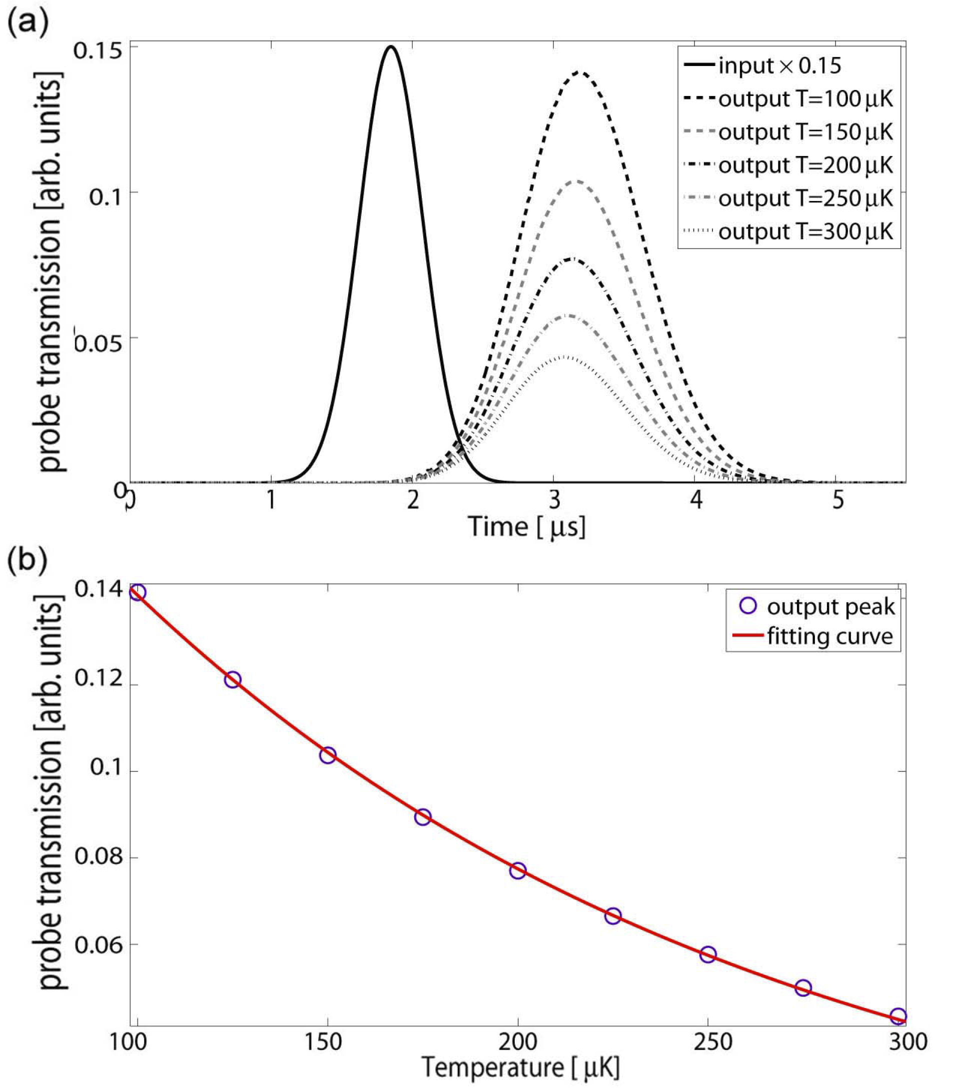
Figure 4: (Color online) The best fitting of the numerical simulation with $\Omega_{c}=$ $0.825\Gamma$, $OD=30$, $T=240$ $\mu$K for LS. The squares and circles are the experimentally measured intensities of the input probe pulse and output probe pulse, respectively. The dashed line and solid line represent the the nurmerical simulations for the intensities of the input probe pulse and output probe pulse, respectively. The input probe pulse is scaled down by a factor of $0.05$.

The influence of the thermal effect is readily revealed by the considerably diminished intensity of the output probe beam. In Fig.4(a), the intensity profiles of the output probe pulse at various temperatures are shown for SL. As expected, the output intensity decreases when the temperature increases. A simple explanation for this is that the higher the temperature, the broader the velocity distribution is. Thus the effective two-photon detuning (the averaged Doppler shift) becomes larger and the output probe pulse is significantly suppressed. Fig.4(b) shows that the peak of the output probe decays exponentially as a function of temperature.

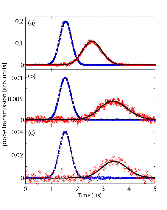
Figure 2: (Color online) The best fitting of the numerical simulation with (a) $\Omega_{c}=0.825\Gamma$, $OD=30$, $T=290$ $\mu$K; (b) $\Omega_{c}=0.665\Gamma$, $OD=41.3$, $T=305$ $\mu$K; (c) $\Omega_{c}=0.75\Gamma$, $OD=48$, $T=280$ $\mu$K for SL. The squares and circles represent the intensities of the experimentally measured input probe pulse and output probe pulse, respectively. The input probe pulse is scaled down by a factor of $0.2$ in (a), $0.01$ in (b) and $0.04$ in (c), respectively. The dashed and solid lines represent the nurmerical simulations for the intensities of the input probe pulse and the output probe pulse, respectively.

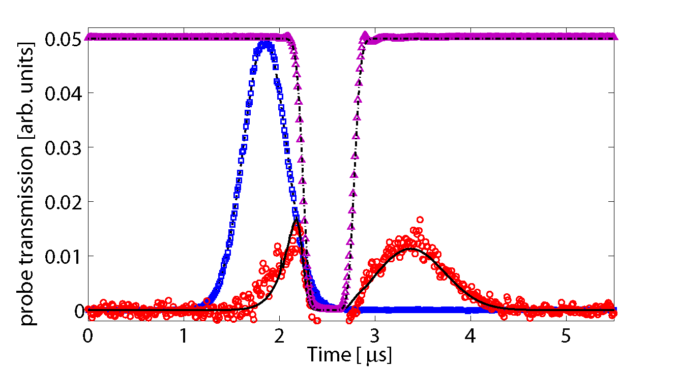
Figure 3: (Color online) The best fitting of the numerical simulation with $\Omega_{c}=$ $0.825\Gamma$, $OD=30$, $T=240$ $\mu$K for LS. The squares and circles are the experimentally measured intensities of the input probe pulse and output probe pulse, respectively. The dashed line and solid line represent the the nurmerical simulations for the intensities of the input probe pulse and output probe pulse, respectively. The input probe pulse is scaled down by a factor of $0.05$.

For all practical purposes, it is more instructive to examine the ground-state coherence, $\left\langle\rho_{21}\right\rangle_{T}$ , rather than the output intensity of the probe beam, since there are no light fields during the process of storage, and once the stored pulse is retrieved, it restores SL again. Although $\left\langle\rho_{21}\right\rangle_{T}$ can not be measured directly, its magnitude determines the intensity of the retrieved probe pulse when the coupling field is turned off. Very recently, in analyzing the feasibility of measuring the ground-state coherence in an EIT, Zhao et al. Bo Zhao suggested that $\left\langle\rho_{21}\right\rangle_{T}$ decays like a Gaussian function during LS. On this basis, it can be further shown that

$$\left\langle\rho_{21}\left(z,t\right)\right\rangle_{T}=\left\langle\rho_{21}(z,t=0)\right\rangle_{T}e^{-(kv_{s})^{2}t^{2}}e^{2ikz},$$ (26)

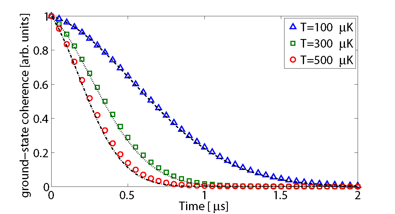
Figure 5: (Color online) The triangles, squares and circles are the numerical results of the normalized $R_{21}(t,T)$ during the storage at $T=100$, $300$ and $500$ $\mu$K, respectively; the dashed-dotted, dotted and dashed lines are the predictions by eq.(26).

where $v_{s}=\sqrt{2k_{B}T/m}$ is the one-dimensional root-mean-square velocity and $k=c^{-1}(\omega_{3}-\omega_{1})$. Now let us consider the case of the storage time of $1.4$ $\mu$s for various temperatures $T=100,300,500$ $\mu$K. In the calculation, the probe pulse enters the medium under $\Omega_{c}=0.75\Gamma$ and $OD=32$ both of which do not affect the decay behavior during the storage; the input probe pulse and the timing of switching off the coupling field are the same as those shown in Fig.3. For such a storage time and atom temperatures the atomic thermal motion is expected to well smear the quantum memory of the probe pulse which is stored as the ground-state coherence. Because eq.(26) is a function of $z$ and $t$ and the time-dependence only comes from the Gaussian function, to eliminate the $z$ dependence of the ground-state coherence, we plot the function $R_{21}\left(t,T\right)=\left|\int\left\langle\rho_{21}\left(z,t\right)\right\rangle_{T}dz\right|$ in Fig.5. We see that the $R_{21}\left(t,T\right)$ indeed decays Gaussian-like with time as predicted in Bo Zhao . Now let us denote $\tau$ as the $1/e$ width of the Gaussian function. Accordingly, $\tau$ of the fitted Gaussian function of the ground-state coherence in the simulation is found to be close to the value predicted by eq.(26). Furthermore, we have verified that $\tau\propto T^{-1/2}$, and the close agreement with the theoretical predictions of eq.(26) are also shown in Fig.5. Since the thermal motion would randomize the spatial profile of the ground-state coherence during the storage, the intensity of the retrieved probe pulse is thus much smaller than the stored one as shown in Fig.3.

The ground-state coherence for SL can be studied in a similar manner. It is expected that the ground-state coherence decays more slowly in SL than in LS, since the continuous optical excitations from the coupling field can retard the loss of atomic coherence led by the randomization of atoms’ thermal motion. We simulate the process of SL with $\Omega_{c}=$ $0.75\Gamma$, and $OD=400$ at various temperatures. Here we have chosen a very large optical density $OD=400$ to ensure that the probe pulse can stay in the medium for a sufficiently long period. We plot $R_{21}\left(t,T\right)$ as a function of time for various temperatures after the probe pulse has entirely merged into the medium, and the numerical results suggest that $R_{21}\left(t,T\right)$ decays exponentially with a rate $\kappa$. In the following, we apply some previous theoretical results based on the steady-state solution of the optical-Bloch equation to derive an analytic estimate of $\kappa$. For simplicity, we shall assume that the EIT transparency bandwidth is much larger than the frequency bandwidth of the probe pulse, such that the decay of the probe pulse or the ground-state coherence is mainly determined by the absorption in the center of the transparency window of the EIT spectrum. Because all decoherence mechanisms other than the atomic thermal motion are neglected, the steady-state solution of $\rho_{31}$ of a rest EIT medium is given by Chen

$$\frac{\rho_{31}}{\Omega_{p}}=\frac{\triangle_{c}-\triangle_{p}}{\Omega_{c}^{2}/2+2[\triangle_{p}-i\Gamma/2][\triangle_{c}-\triangle_{p}]}.$$ (27)

Given that the probe and coupling fields are both resonant with the atomic transition frequencies in the laboratory frame, thus for an atom moving with a velocity $v$, we have $\triangle_{p}=kv$ and $\triangle_{c}=-kv$ in the above equation. In the presence of a strong coupling field, $\Omega_{c}\gg kv_{s}$, the imaginary part of eq.(27) can be approximated by

$$\textit{Im}\left[\frac{\rho_{31}(v)}{\Omega_{p}}\right]\approx\frac{4k^{2}v^{2}\Gamma}{\Omega_{c}^{4}},$$ (28)

which is related to the absorption coefficient $\alpha$ of a Doppler-broadened medium by

$$\alpha=\eta\left\langle\textit{Im}\left[\frac{\rho_{31}(v)}{\Omega_{p}}\right]\right\rangle_{T}=\frac{4\eta k^{2}v_{s}^{2}\Gamma}{\Omega_{c}^{4}}.$$ (29)

The absorption gives rise to the attenuation of the propagating light pulse, that is described by the Beer’s law, namely,

$$\frac{R_{21}\left(t,T\right)}{R_{21}\left(0,T\right)}=e^{-2\alpha l}=e^{-2\alpha v_{g}t},$$ (30)

where $l$ is the propagation distance and $v_{g}=\Omega_{c}^{2}/2\eta$ is the group velocity. It is straightforward to obtain $\kappa=4\left(kv_{s}/\Omega_{c}\right)^{2}\Gamma$ with eq.(30). In contrast to the Gaussian decay in eq.(26), which depends on temperature only, the decay of ground-state coherence in SL depends on the temperature, coupling field and the spontaneous decay rate of level $\left|3\right\rangle$. The numerical simulations of $R_{21}\left(t,T\right)$ and the analytic predictions are plotted for various temperatures in Fig.6, where good agreements are demonstrated. It is not unexpected that our numerical simulations closely agree with those obtained by averaging the solutions of optical-Bloch equations subjected to the Maxwell-Boltzmann distribution at a particular temperature, since in our numerical calculations so far, the effect of recoil is negligible, i.e., $\left(k_{p}-\tilde{k}_{c}\right)v_{s}\gg\hbar(k_{p}-\tilde{k}_{c})^{2}/2m$ [see the definition of $\triangle_{v}$ below eq.(II)]. However, we note that the above criterion is no longer valid if the mass of atom is made small and the coupling and probe beams are counter-propagating. The resultant dephasing can significantly reduce the output level of the probe pulse and our scheme appears applicable to this kind of problems.

Finally, it should be noted that, simply by adjusting the temperature (or equivalently, the velocity distribution), we can simulate the decaying behavior of the ground-state coherence, provided that the explicit time-dependence of the coupling field is given. This can not be achieved via solving the optical-Bloch equation by imposing a phenomenological decay rate $\gamma$ on the metastable ground state $\left|2\right\rangle$ (which is accurate only at $\Omega_{c}\gg kv_{s}$ in SL and not valid at all in LS), and thus features the major decoherence between our formalism and the optical-Bloch equation. For this reason, it is expected that the current scheme can be applied to investigate the dynamics of stationary light pulse (SLP) which is basically consisted of four SL processes — two co-propagating and two counter-propagating. Owing to the inherent complexity, specifying the high-order $\gamma$’s in the SLP turns out to be tricky when solving the usual optical Bloch equations Pan . Under the circumstances, without doubt, our scheme appears to be an easier and more natural way to approach the problem.

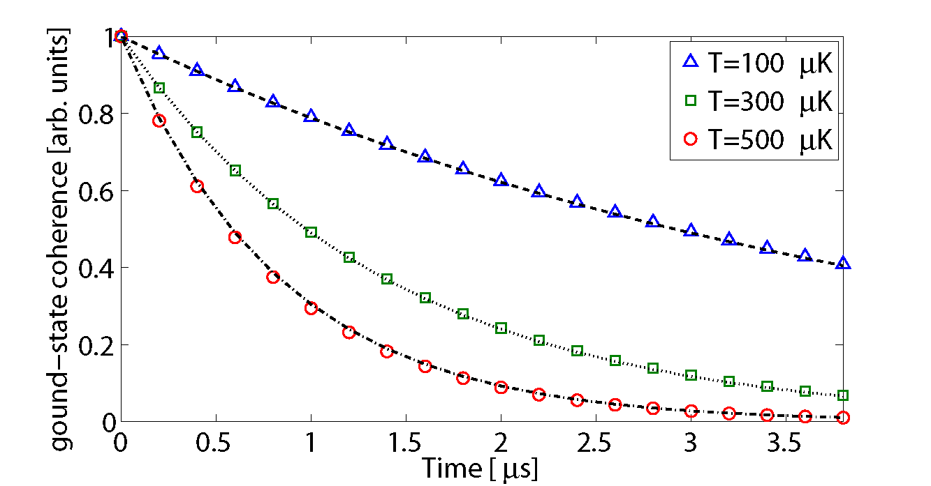
Figure 6: (Color online) The normalized $R_{21}\left(t,T\right)$ with $\Omega_{c}=$ $0.75\Gamma$, $OD=400$; the triangles, squares and circles are the numerical results at $T=100$, $300$ and $500\mu$K, respectively; the dashed-dotted, dotted and dashed lines are the predictions of eq.(30).

IV Concluding remarks

We have presented a numerical scheme to study the dynamics of SL and LS in an EIT medium at finite temperatures. Based on the gauge invariance of Schrödinger equation under Galilean transformation, we derive a set of coupled equations for a boosted closed 3-level EIT systems. The loss of ground-state coherence at finite temperatures is then treated as a consequence of superposition of density matrices representing the EIT systems moving at different velocities. Unlike other theoretical treatments in which atoms are assumed immobile, our scheme takes both atom’s external and internal degrees of freedom into full account. The feasibility of this scheme is shown by comparing the numerical results to the experimental data for both SL and LS. Last but not least, this scheme also enables us to study the dynamical properties of a Doppler-broadened EIT medium in the non-perburbative regime of probe and coupling pulses with comparable intensities, in which new effects are expected to arise.

ACKNOWLEDGEMENTS

This work is supported in part by National Science Council, Taiwan under Grant No. 98-2112-M-018-001-MY2 and 98-2628-M-007-001. TLH and SCG acknowledge the supports from Taida Institute for Mathematical Science (TIMS) and the National Center for Theoretical Sciences (NCTS).

References

- (1) M. Fleischhauer, A. Imamoğlu, and J. P. Marangos, Rev. Mod. Phys. 77, 633 (2005), and references therein.
- (2) S. E. Harris and L. V. Hau, Phys. Rev. Lett. 82, 4611 (1999).
- (3) K.-J. Boller, A. Imamoğlu, and S. E. Harris, Phys. Rev. Lett. 66, 2593 (1991).
- (4) J. E. Field, K. H. Hahn, and S. E. Harris, Phys. Rev. Lett. 67, 3062 (1991).
- (5) L. V. Hau, S. E. Harris, Z. Dutton, and C. H. Behroozi, Nature (London) 397, 594 (1999).
- (6) D. D. Budker, D. F. Kimball, S. M. Rochester, and V. V. Yashchuk, Phys. Rev. Lett. 83, 1767 (1999).
- (7) M. Fleishhauer and M. D. Lukin, Phys. Rev. Lett. 84, 5094 (2000).
- (8) C. Liu, Z. Dutton, C. H. Behroozi, and L. V. Hau, Nature (London) 409, 490 (2001).
- (9) M. M. Kash, V. A. Sautenkov, A. S. Zibrov, L. Hollberg, G. R. Weich, M. D. Lukin, Y. Rostovtsev, E. S. Fry, and M. O. Scully, Phys. Rev. Lett. 82, 5229 (1999).
- (10) A. Javan, O. Kocharovskaya, H. Lee, and M. O. Scully, Phys. Rev. A 66, 013805 (2002).
- (11) D. F. Phillips, A. Fleischhauer, A. Mair, R. L.Walsworth, and M. D. Lukin, Phys. Rev. Lett. 86, 783 (2001).
- (12) O. Kocharovskaya, U. Rostovtsev, and M. O. Scully, Phys. Rev. Lett. 86, 628 (2001).
- (13) A. V. Turukhin, V. S. Sudarhanam, M. S. Shariar, J. A. Musser, B. S. Ham, and P. R. Hemmer, Phys. Rev. Lett. 88, 02362 (2001).
- (14) L.-M. Duan, J. I. Cirac, and P. Zoller, Science 292, 1695 (2001).
- (15) T. Chaneliere, D. N. Matsukevich, S. D. Jenkins, S.-Y. Lan, T. A. B. Kennedy, and A. Kuzmich, Nature (London) 438, 833 (2005).
- (16) F. Vewinger, J. Appel, E. Figuera, and A. Lvovsky, Opt. Lett. 32, 2771 (2007).
- (17) Y. W. Lin, W. T. Liao, T. Peters, H. C. Chou, J. S. Wang, H. W. Cho, P. C. Kuan and I. A. Yu, Phys. Rev. Lett. 102, 213601 (2009).
- (18) T. Peters, Y. H. Chen, J. S. Wang, Y. W. Lin, and I. A. Yu, Opt. Lett. 35, 151 (2010).
- (19) B. Zhao, Y.-A. Chen, X.-H. Bao, T. Strassel, C.-S. Chuu, X.-M. Jin, J. Schmiedmayer, Z.-S. Yuan, S. Chen and J.-W. Pan, Nature Phys. 5, 95 (2008).
- (20) M. O. Scully and M. S. Zubairy, Quantum Optics (Cambridge University Press, Cambridge, U.K., 1997).
- (21) E. Merzbacher, Quantum Mechanics (John Wiley & Sons, 1998).
- (22) Y. W. Lin, H. C. Chou, P. P. Dwivedi, Y.-C. Chen, and I. A. Yu, Opt. Express 16, 3753 (2008).
- (23) J. H. Wu, M. Artoni, and G. C. LaRocca, Phys. Rev. A 82, 013807 (2010).
- (24) Y.-F. Chen, Y.-M. Kao, W.-H. Lin and I. A. Yu, Phys. Rev. A 74, 063801 (2006).
- (25) R. Wei, B. Zhao, Y. Deng, S. Chen, Z.-B. Chen and J.-W. Pan, Phys. Rev. A 81, 043403 (2010).