Second-order nonadiabatic couplings from time-dependent density functional theory: Evaluation in the immediate vicinity of Jahn-Teller/Renner-Teller intersections

Abstract

For a rigorous quantum simulation of nonadiabatic dynamics of electrons and nuclei, knowledge of not only first-order but also second-order nonadiabatic couplings (NAC), is required. Here we propose a method to efficiently calculate second-order NAC from time-dependent density functional theory (TDDFT), on the basis of the Casida ansatz adapted for the computation of first-order NAC, which has been justified in our previous work and can be shown to be valid for calculating second-order NAC between ground state and singly excited states within the Tamm-Dancoff approximation. Test calculations of second-order NAC in the immediate vicinity of Jahn-Teller and Renner-Teller intersections show that calculation results from TDDFT, combined with modified linear response theory, agree well with the prediction from the Jahn-Teller / Renner-Teller models. Contrary to the diverging behavior of first-order NAC near all types of intersection points, the Cartesian components of second-order NAC are shown to be negligibly small near Renner-Teller glancing intersections, while they are significantly large near the Jahn-Teller conical intersections. Nevertheless, the components of second-order NAC can cancel each other to a large extent in Jahn-Teller systems, indicating the background of neglecting second-order NAC in practical dynamics simulations. On the other hand, it is shown that such a cancellation becomes less effective in an elliptic Jahn-Teller system and thus the role of second-order NAC needs to be evaluated in the rigorous framework. Our study shows that TDDFT is promising to provide accurate data of NAC for full quantum mechanical simulation of nonadiabatic processes.

I Introduction

Nonadiabatic transitions, i.e., transitions between adiabatic states, are ubiquitous in physical, chemical and biological systems. Yarkony (1996); Nakamura (2002); Baer (2006) In recent years there has been growing interest in quantum mechanical study of nonadiabatic transitions,Doltsinis and Marx (2002); Li et al. (2005); Isborn et al. (2007); Martínez (1997); Yonehara and Takatsuka (2008a, b) which has been regarded as a challenging field for theorists: Although most ab initio theories are built upon the Born-Oppenheimer approximation to separate the nuclear and electronic degrees of freedom, this approximation will break down in the region where nonadiabatic transitions occur. In order to describe nonadiabatic processes, it is necessary to go beyond the Born-Oppenheimer approximation and take account of nonadiabatic couplings (NAC), which is the driving force for nonadiabatic transition to different potential energy surfaces (PES). Baer (2006) Since NAC (preferentially called as first and second derivative couplings in quantum chemistry) are defined as matrix elements of the first and second derivatives with respect to nuclear coordinates between adiabatic states (many-body wavefunctions), nonadiabatic dynamics simulation has long been relying on wavefunction-based methods to provide the NAC data. For more efficient calculation of NAC, density functional methods, Billeter and Curioni (2005) especially those based on time-dependent density functional theory (TDDFT), have been developed in the last decade. The study was initiated by Chernyak and Mukamel Chernyak and Mukamel (2000) who proposed to perturb the ground state using the nuclear derivative of Hamiltonian and to compute NAC from the density response. This scheme was first implemented by Baer Baer (2002) to study H₃ using a real-time approach and by Hu et al. Hu et al. (2007, 2008) to systematically study small molecules using the frequency-space formalism of Casida. cas ; Jamorski et al. (1996) To avoid the pseudopotential problem in the calculation of NAC, all-electron TDDFT schemes have been independently developed by Hu et al. Hu et al. (2009) and Send et al. Send and Furche (2010) Alternatively, formulations of NAC from TDDFT has also been achieved by Tavernelli et al. Tapavicza et al. (2007); Tavernelli et al. (2009a, 2010a) using the Casida ansatz, which is promising to correctly give NACs between excited states within the Tamm-Dancoff approximation (TDA). A recent study by Hu et al. Hu et al. (2010) further clarified relationships between different DFT/TDDFT formulations of NAC. Billeter and Curioni (2005); Tapavicza et al. (2007); Tavernelli et al. (2009b, 2010b) These NAC schemes have been applied to nonadiabatic dynamics simulations and have shown that TDDFT is promising for balanced cost and performance on the computation of polyatomic systems. Tapavicza et al. (2007, 2008); Werner et al. (2008); Hirai and Sugino (2009)

So far most studies on the computation and application of NAC are focused on the first-order, without much discussion on the second-order. Although second-order NAC can be in principle expressed by the first-order, the numerical evaluation can not be easily carried out. This is because not only the differentiation of first-order NAC is needed, but also a complete expansion in eigenstates makes the product of first-order NAC involving these states rather complicated. In the wavefunction-based framework, although several methods for evaluating second-order NAC have been presented, Redmon (1982); Lengsfield III et al. (1986); Ågren et al. (1986) there are very few literatures on the direct evaluation of second-order NAC in molecular systems. Correspondingly, the practical study by nonadiabatic simulation seldom takes second-order NAC into consideration. A simplified procedure is to replace the full quantum description as the quantum-classical simulation, since the time evolution of the nuclear degrees of freedom is described by a Poisson bracket that introduces only first order derivatives. Santer et al. (2001) On the other hand, even the full nonadiabatic operators, both first- and second-order NAC, are taken into consideration in the formulation, such as ab initio multiple spawning, the second-order NAC are just ignored in the practice. Martínez (1997); Martínez et al. (1997); Ben-Nun and Martínez (1998) It is noted that second-order NAC are often found to be small by experience, Martínez (1997) however, they are not the second-order item in the Taylor expansion but originated from the presence of the scalar Laplacian. Therefore, in contrast to the vector form of first-order NAC, the second order are scalars. In order to verify the validity of neglecting second-order NAC in nonadiabatic simulations, it is crucial to examine the behavior of second-order NAC when the intersection points are approached. If the similar diverging behavior as first-order NAC is observed, the neglect of second-order NAC needs to be critically reconsidered.

The aim of the present study is to develop an efficient TDDFT method for the calculation of second-order NAC, which is desired to have the same-level computational cost as the first-order, and then to examine the behavior of second-order NAC near intersection points. For the efficiency, the explicit expansion into first-order NAC should be avoided. We will show that this can be achieved by using the Casida ansatz adapted for the first-order NAC, Hu et al. (2010) while there is no need to explicitly construct auxiliary excited-state wavefunctions. Tavernelli et al. (2009b) Justification of our procedure can be shown within the TDA. To check if the second-order NAC diverge at intersection points, we carry out TDDFT calculations within modified linear response theory Hu et al. (2006); Hu and Sugino (2007) in the immediate vicinity of Jahn-Teller,Bersuker (2001, 2006) Renner-Teller Jungen and Merer (1980); Mikhailov et al. (2006) and elliptic Jahn-Teller intersections, Vibók et al. (2003) and compare results with model analysis. It is verified that our TDDFT results are in good agreement with the predictions from the models. In the vicinity of different types of intersections different behaviors of second-order NAC are revealed, either in the Cartesian components ($x$, $y$ and $z$) or as a whole scalar: The components are shown to be negligibly small near Renner-Teller glancing intersections, while they are significantly large near the Jahn-Teller conical intersections. Nevertheless, the components of second-order NAC can cancel each other to a large extent in Jahn-Teller systems, indicating the background of neglecting second-order NAC in practical dynamics simulations. On the other hand, it is also shown that such a cancellation becomes less effective in an elliptic Jahn-Teller system and thus the role of second-order NAC needs to be evaluated in the rigorous framework.

The present paper is organized as follows. In Sec. II, we present the formulation of second-order NAC from TDDFT and its extension within modified linear response theory. In Sec. III, implementation in the planewave pseudopotential framework and computational details are given. In Sec. IV, practical calculations on various molecular systems possessing Jahn-Teller, Renner-Teller or elliptic Jahn-Teller intersections are performed, and compared with ideal values predicted by Jahn-Teller / Renner-Teller models. In Sec. V, we conclude our work.

II Formulation

II.1 Second-order NAC from the adapted Casida ansartz

In the previous work of Hu et al. rigorous TDDFT formulations of first-order NAC have been achieved, using the Kohn-Sham matrix elements of either $h$-operator Hu et al. (2007, 2008, 2009) or $d$-operator, Hu et al. (2010) i.e.,

$$\hat{h}_{\mu}\equiv\frac{\partial\hat{H}}{\partial R_{\mu}},\quad\quad\hat{d}_{\mu}\equiv\frac{\partial}{\partial R_{\mu}},$$ (1)

where $H$ is the many-body Hamiltonian and $R_{\mu}$ is the nuclear coordinate with $\mu$ representing $x$, $y$, and $z$ components and atom index.

The $h$-matrix formulation gives first-order NAC as

$$\left\langle\Psi_{0}\right|\frac{\partial}{\partial R_{\mu}}\left|\Psi_{I}\right\rangle=\omega_{I}^{-1}\left\langle\Psi_{0}\right|\frac{\partial\hat{H}}{\partial R_{\mu}}\left|\Psi_{I}\right\rangle=\omega_{I}^{-3/2}\mathbf{h}_{\mu}^{\dagger}\mathbf{S}^{-1/2}\mathbf{F}_{I}.$$ (2)

where $\Psi_{0}$ ($\Psi_{I}$) is the many-body electronic wavefunction of the ground ($I$-th excited) state, and $\omega_{I}$ is the excitation energy. Matrix elements of $\mathbf{S}$ and $\mathbf{h}_{\mu}$ are given by

$$S_{ij\sigma,kl\tau}=\frac{\delta_{\sigma,\tau}\delta_{i,k}\delta_{j,l}}{\left(f_{k\tau}-f_{l\tau}\right)\left(\varepsilon_{l\tau}-\varepsilon_{k\tau}\right)}$$ (3)

and

$$h_{ij\sigma,\mu}=\left\langle\psi_{i\sigma}\right|\frac{\partial\hat{H}}{\partial R_{\mu}}\left|\psi_{j\sigma}\right\rangle,$$ (4)

where $\psi_{i\sigma}$, $\varepsilon_{i\sigma}$, $f_{i\sigma}$ are, respectively, the orbital, eigenvalue, and occupation number for the $i$-th KS state with spin $\sigma$. $\mathbf{F}_{I}$ is the eigenvector of the Casida equation cas

$$\mathbf{\Omega F}_{I}=\omega_{I}^{2}\mathbf{F}_{I},$$ (5)

where

$$\Omega_{ij\sigma,kl\tau}=\delta_{\sigma,\tau}\delta_{i,k}\delta_{j,l}\left(\varepsilon_{l\tau}-\varepsilon_{k\tau}\right)^{2}+2\sqrt{\left(f_{i\sigma}-f_{j\sigma}\right)\left(\varepsilon_{j\sigma}-\varepsilon_{i\sigma}\right)}K_{ij\sigma,kl\tau}\sqrt{\left(f_{k\tau}-f_{l\tau}\right)\left(\varepsilon_{l\tau}-\varepsilon_{k\tau}\right)}$$ (6)

with $\mathbf{K}$ being the KS matrix of the Hartree and exchange-correlation (xc) kernel ($\Lambda^{\text{hxc}}$),

$$K_{ij\sigma,kl\tau}=\int\int d\mathbf{r}d\mathbf{r}^{\prime}\psi_{i\sigma}\left(\mathbf{r}\right)\psi_{j\sigma}\left(\mathbf{r}\right)\Lambda^{\text{hxc}}\left(\mathbf{r},\mathbf{r}^{\prime}\right)\psi_{k\tau}\left(\mathbf{r}^{\prime}\right)\psi_{l\tau}\left(\mathbf{r}^{\prime}\right).$$ (7)

The KS orbitals have been assumed to be real for simplicity.

On the other hand, the $d$-matrix formulation gives first-order NAC as

$$\left\langle\Psi_{0}\right|\frac{\partial}{\partial R_{\mu}}\left|\Psi_{I}\right\rangle=\omega_{I}^{1/2}\mathbf{d}_{\mu}^{\dagger}\mathbf{S}^{1/2}\mathbf{F}_{I},$$ (8)

where

$$d_{ij\sigma,\mu}=\left\langle\psi_{i\sigma}\right|\hat{d}_{\mu}\left|\psi_{j\sigma}\right\rangle=\left\langle\psi_{i\sigma}\right|\frac{\partial}{\partial R_{\mu}}\left|\psi_{j\sigma}\right\rangle.$$ (9)

The $d$-matrix formulation is derived from the original $h$-matrix formulation, using the relationship between the nuclear derivatives of many-body Hamiltonian and Kohn-Sham Hamiltonian. It can avoid the problem of the pseudopotential approximation in reproducing the inelastic terms corresponding to the off-diagonal $h$-matrix elements.

It is interesting to note that the two TDDFT formulations of first-order NAC, Eqs. (2) and (8), give similar but subtly different expressions for the connection between TDDFT quantities and many-body theory, i.e.,

$$\mathbf{h}_{\mu}^{\dagger}\mathbf{S}^{-1/2}\mathbf{F}_{I}=\omega_{I}^{1/2}\left\langle{\Psi}_{0}\right|\hat{h}_{\mu}\left|{\Psi}_{I}\right\rangle$$ (10)

and

$$\mathbf{d}_{\mu}^{\dagger}\mathbf{S}^{1/2}\mathbf{F}_{I}=\omega_{I}^{-1/2}\left\langle{\Psi}_{0}\right|\hat{d}_{\mu}\left|{\Psi}_{I}\right\rangle,$$ (11)

which can be further compared with the one for the dipole operator $\hat{r}_{\mu}$,

$$\mathbf{r}_{\mu}^{\dagger}\mathbf{S}^{-1/2}\mathbf{F}_{I}=\omega_{I}^{1/2}\left\langle{\Psi}_{0}\right|\hat{r}_{\mu}\left|{\Psi}_{I}\right\rangle,$$ (12)

as derived by Casida for the calculation of oscillator strength. cas The expression of the $\hat{d}_{\mu}$ operator, Eq. (11), shows a distinct feature as it gives different powers in $\mathbf{S}$ and $\omega_{I}$. It is reminded that Eq. (12) is the basis of the Casida ansatz, in which the auxiliary many-body excited-state wavefunction is constructed as

$$\bar{\Psi}_{I}=\sum_{ij\sigma}^{f_{i\sigma}>f_{j\sigma}}\sqrt{\frac{\varepsilon_{j\sigma}-\varepsilon_{i\sigma}}{\omega_{I}}}F_{ij\sigma,I}\hat{a}_{j\sigma}^{\dagger}\hat{a}_{i\sigma}\bar{\Psi}_{0},$$ (13)

so that

$$\left\langle{\Psi}_{0}\right|\hat{O}_{\mu}\left|{\Psi}_{I}\right\rangle=\left\langle\bar{\Psi}_{0}\right|\hat{O}_{\mu}\left|\bar{\Psi}_{I}\right\rangle.$$ (14)

Herein $\hat{a}_{j\sigma}^{\dagger}$ and $\hat{a}_{i\sigma}$ are respectively creation and annihilation operators, and $\bar{\Psi}_{0}$ is a Slater determinant of occupied KS orbitals. Details regarding the Casida ansatz and the mapping between TDDFT quantities and many-body theory can be found in Ref. [Tavernelli et al., 2009b]. Nevertheless, in order to validate Eq. (14) also for $\hat{O}_{\mu}$ = $\hat{d}_{\mu}$, the Casida ansatz need to be adapted according to Eq. (11) in the following way,

$$\tilde{\Psi}_{I}=\sum_{ij\sigma}^{f_{i\sigma}>f_{j\sigma}}\sqrt{\frac{\omega_{I}}{\varepsilon_{j\sigma}-\varepsilon_{i\sigma}}}F_{ij\sigma,I}\hat{a}_{j\sigma}^{\dagger}\hat{a}_{i\sigma}\tilde{\Psi}_{0},$$ (15)

where $\tilde{\Psi}_{0}=\bar{\Psi}_{0}$.

With the adapted Casida ansatz in hand, we can now readily derive the second-order NAC, assuming the similarity between first- and second-derivative operators. Defining

$$\hat{b}_{\mu}\equiv\frac{\partial^{2}}{\partial R_{\mu}^{2}},$$ (16)

we can get

$$\left\langle{\Psi}_{0}\right|\hat{b}_{\mu}\left|{\Psi}_{I}\right\rangle=\left\langle\tilde{\Psi}_{0}\right|\hat{b}_{\mu}\left|\tilde{\Psi}_{I}\right\rangle.$$ (17)

from the adapted Casida ansatz. Since Eq. (15) is equivalent to

$$\tilde{\Psi}_{I}=\sum_{ij\sigma}^{f_{i\sigma}>f_{j\sigma}}\omega_{I}^{1/2}\left(\mathbf{S}^{1/2}\mathbf{F}_{I}\right)_{ij\sigma}\hat{a}_{j\sigma}^{\dagger}\hat{a}_{i\sigma}\tilde{\Psi}_{0},$$ (18)

further using the connection from the Casida ansatz to the mapping between TDDFT and many-body theory Tavernelli et al. (2009b), we can get

$$\mathbf{b}_{\mu}^{\dagger}\mathbf{S}^{1/2}\mathbf{F}_{I}=\omega_{I}^{-1/2}\left\langle{\Psi}_{0}\right|\hat{b}_{\mu}\left|{\Psi}_{I}\right\rangle,$$ (19)

i.e.,

$$\left\langle{\Psi}_{0}\right|\frac{\partial^{2}}{\partial R_{\mu}^{2}}\left|{\Psi}_{I}\right\rangle=\omega_{I}^{1/2}\mathbf{b}_{\mu}^{\dagger}\mathbf{S}^{1/2}\mathbf{F}_{I}.$$ (20)

This expression shows that we can calculate second-order NAC without explicitly constructing (auxiliary) excited wavefunctions. Moreover, it is appealing that the computational cost of second-order NAC by this expression is at the same-level as that of the first-order. On the other hand, it is noted that although the derivation of Eq. (11) is rigorous, derivation of Eq. (19) is not yet. The validity of the adapted Casida ansatz for the second-order NAC needs to be further justified. Next we show that this can be achieved within the TDA, where the adapted Casida ansatz becomes equivalent to the original one.

II.2 Second-order NAC within the TDA

The justification of the second-order NAC formulation can be attempted by using the expansion of first-order NAC to show the validity of Eq. (17). It has been shown Hu et al. (2010); Tavernelli et al. (2010a) that for those between ground state and singly excited states, it generally holds that

$$\left\langle{\Psi}_{0}\right|\hat{d}_{\mu}\left|{\Psi}_{I}\right\rangle=\left\langle\tilde{\Psi}_{0}\right|\hat{d}_{\mu}\left|\tilde{\Psi}_{I}\right\rangle,$$ (21)

and for those between singly excited states, the validity of the expression

$$\left\langle{\Psi}_{I}\right|\hat{h}_{\mu}\left|{\Psi}_{J}\right\rangle=\left\langle\bar{\Psi}_{I}\right|\hat{h}_{\mu}\left|\bar{\Psi}_{J}\right\rangle$$ (22)

can be justified using the TDA, where $\omega_{I}^{1/2}\mathbf{S}^{1/2}=1$, and the two forms of auxiliary wavefunctions become the same, i.e., $\bar{\Psi}_{I}=\tilde{\Psi}_{I}$. The second-order NAC can be expanded by the first-order as

$$\left\langle{\Psi}_{0}\right|\hat{b}_{\mu}\left|{\Psi}_{I}\right\rangle=-\langle\frac{\partial}{\partial R_{\mu}}\Psi_{0}|\frac{\partial}{\partial R_{\mu}}\Psi_{I}\rangle+\frac{\partial}{\partial R_{\mu}}\left\langle{\Psi}_{0}\right|\frac{\partial}{\partial R_{\mu}}\left|{\Psi}_{I}\right\rangle\\ =-\sum_{m}\langle\frac{\partial}{\partial R_{\mu}}\Psi_{0}|\Psi_{m}\rangle\langle\Psi_{m}|\frac{\partial}{\partial R_{\mu}}\Psi_{I}\rangle+\frac{\partial}{\partial R_{\mu}}\left\langle{\Psi}_{0}\right|\frac{\partial}{\partial R_{\mu}}\left|{\Psi}_{I}\right\rangle\\ =\sum_{m}\left\langle{\Psi}_{0}\right|\hat{d}_{\mu}\left|{\Psi}_{m}\right\rangle\frac{\left\langle{\Psi}_{m}\right|\hat{h}_{\mu}\left|{\Psi}_{I}\right\rangle}{E_{I}-E_{m}}+\frac{\partial}{\partial R_{\mu}}\left\langle{\Psi}_{0}\right|\hat{d}_{\mu}\left|{\Psi}_{I}\right\rangle,$$ (23)

which rigorously holds since $\langle\Psi_{m}|\Psi_{n}\rangle=\delta_{mn}$. Similarly, if we can show this orthonormalized condition for the auxiliary wavefunction, i.e., $\langle\tilde{\Psi}_{m}|\tilde{\Psi}_{n}\rangle=\delta_{mn}$, we can get

$$\left\langle\tilde{\Psi}_{0}\right|\hat{b}_{\mu}\left|\tilde{\Psi}_{I}\right\rangle=-\langle\frac{\partial}{\partial R_{\mu}}\tilde{\Psi}_{0}|\frac{\partial}{\partial R_{\mu}}\tilde{\Psi}_{I}\rangle+\frac{\partial}{\partial R_{\mu}}\left\langle\tilde{\Psi}_{0}\right|\frac{\partial}{\partial R_{\mu}}\left|\tilde{\Psi}_{I}\right\rangle\\ =-\sum_{m}\langle\frac{\partial}{\partial R_{\mu}}\tilde{\Psi}_{0}|\tilde{\Psi}_{m}\rangle\langle\tilde{\Psi}_{m}|\frac{\partial}{\partial R_{\mu}}\tilde{\Psi}_{I}\rangle+\frac{\partial}{\partial R_{\mu}}\left\langle\tilde{\Psi}_{0}\right|\frac{\partial}{\partial R_{\mu}}\left|\tilde{\Psi}_{I}\right\rangle\\ =\sum_{m}\left\langle\tilde{\Psi}_{0}\right|\hat{d}_{\mu}\left|\tilde{\Psi}_{m}\right\rangle\frac{\left\langle\tilde{\Psi}_{m}\right|\hat{h}_{\mu}\left|\tilde{\Psi}_{I}\right\rangle}{E_{I}-E_{m}}+\frac{\partial}{\partial R_{\mu}}\left\langle\tilde{\Psi}_{0}\right|\hat{d}_{\mu}\left|\tilde{\Psi}_{I}\right\rangle.$$ (24)

From Eq. (21) and Eq. (22), the identity of Eq. (23) and Eq. (24) can be justified provided that $\tilde{\Psi}_{I}=\bar{\Psi}_{I}$, since we have to reconstruct the auxiliary wavefunction from $\tilde{\Psi}_{m}$ to $\bar{\Psi}_{m}$ when the operator is changed from $\hat{d}_{\mu}$ to $\hat{h}_{\mu}$. This is satisfied when the TDA is valid. In the meanwhile, the orthonormalized condition that

$$\delta_{IJ}=\langle\tilde{\Psi}_{I}|\tilde{\Psi}_{j}\rangle=\sqrt{\omega_{I}\omega_{J}}\sum_{ij\sigma}\sum_{kl\tau}\left(\mathbf{S}^{1/2}\mathbf{F}_{I}\right)^{\dagger}_{ij\sigma}\left(\mathbf{S}^{1/2}\mathbf{F}_{I}\right)_{kl\tau}\left\langle\tilde{\Psi}_{0}\right|\hat{a}^{\dagger}_{i\sigma}\hat{a}_{j\sigma}\hat{a}^{\dagger}_{l\tau}\hat{a}_{k\tau}\left|\tilde{\Psi}_{0}\right\rangle\\ =\sqrt{\omega_{I}\omega_{J}}\sum_{ij\sigma}\sum_{kl\tau}\left(\mathbf{S}^{1/2}\mathbf{F}_{I}\right)^{\dagger}_{ij\sigma}\left(\mathbf{S}^{1/2}\mathbf{F}_{I}\right)_{kl\tau}\delta_{ik}\delta_{jl}\delta_{\sigma\tau}=\sqrt{\omega_{I}\omega_{J}}\mathbf{F}^{\dagger}_{I}\mathbf{S}\mathbf{F}_{J}$$ (25)

also holds within the TDA since $\mathbf{F}^{\dagger}_{I}\mathbf{F}_{J}=\delta_{IJ}$. Therefore, Eq. (23) and Eq. (24) become identical, i.e., the validity of Eq. (17) is justified within the TDA.

Further remark is on the complete expansion in Eq. (24). As long as we only consider a singly excited state, this does not pose a problem since $\tilde{\Psi}_{0}$ is a single Slater determinant and only the contributions from other singly excited states enter the expansion.

II.3 Extension within TDDFT modified linear response theory: Justification of the Slater transition state method

In the calculation of first-order NAC, a particular example is the case of the Slater transition state method for doublet systems. Billeter and Curioni Billeter and Curioni (2005) has used the following expression,

$$\langle\Psi_{0}|\frac{\partial}{\partial R_{\mu}}|\Psi_{I}\rangle=\langle\psi_{i\sigma}^{m}|\frac{\partial}{\partial R_{\mu}}|\psi_{j\sigma}^{m}\rangle,$$ (26)

where the ($i$,$j$) pair is the particle-hole orbitals responsible for the $I$-th transition, and $m$ denotes the mid-excited state (Slater transition state) in which the particle-hole orbitals are each filled with a half electron. They have found that this expression can give accurate results of first-order NAC between doublet states of molecules at equilibrium geometries, and their approach is further validated by our TDDFT modified linear response theory Hu et al. (2006); Hu and Sugino (2007) and also by our calculations near intersection points. Hu et al. (2010) Next we will show that the extension of TDDFT formulation of second-order NAC within modified linear response theory, is also equivalent to the Slater transition state method for doublet systems.

Within modified linear response, the excitation energy is calculated from the response of the mid-excited state, while other terms in the NAC formula are calculated from that of the pure-state configuration. Hu and Sugino (2007) Corresponding to the mid-excited state of a doublet system, the adapted Casida equation,

$$\mathbf{\Omega}^{m}\mathbf{F}_{I}^{m}=\omega_{I}^{m}\mathbf{F}_{I}^{m}$$ (27)

with the matrix element

$$\Omega_{ij\sigma,kl\tau}^{m}=\delta_{i,k}\delta_{j,l}\delta_{\sigma,\tau}(\epsilon_{j\sigma}^{m}-\epsilon_{i\sigma}^{m})^{2}+2(f_{i\sigma}^{m}-f_{j\sigma}^{m})(\epsilon_{j\sigma}^{m}-\epsilon_{i\sigma}^{m})K_{ij\sigma,kl\tau}^{m},$$ (28)

gives

$$\omega_{I}^{m}=\epsilon_{j\sigma}^{m}-\epsilon_{i\sigma}^{m},$$ (29)

since $f_{i\sigma}^{m}$=$f_{j\sigma}^{m}$ = 0.5 in the mid-excited state of a doublet system, which renders the corresponding off-diagonal elements of $\mathbf{\Omega}$ to be zero. On the other hand, the pure state configuration in the mid-excited state, which uses the occupation number of the ground state while keeping other quantities of the mid-excited state, gives

$$\mathbf{b}_{\mu,p}^{\dagger}\mathbf{S}_{p}^{1/2}\mathbf{F}_{I}^{p}=b_{ij\sigma}^{m}(\epsilon_{j\sigma}^{m}-\epsilon_{i\sigma}^{m})^{-1/2},$$ (30)

due to the fact that $F_{ij\sigma,I}^{p}$ is practically equivalent to 1 and other components of $\mathbf{F}_{I}$ are zero. Therefore,

$$\langle\Psi_{0}|\hat{b}_{\mu}|\Psi_{I}\rangle=(\omega_{I}^{m})^{1/2}\mathbf{b}_{\mu,p}^{\dagger}\mathbf{S}_{p}^{1/2}\mathbf{F}_{I}^{p}=b_{ij\sigma}^{m}=\langle\psi_{i\sigma}^{m}|\frac{\partial^{2}}{\partial R_{\mu}^{2}}|\psi_{j\sigma}^{m}\rangle,$$ (31)

which is just the second-derivative coupling matrix element between the particle-hole orbitals. As a result, the TDDFT formulation of second-order NAC in doublet systems is just reduced to the Slater transition state method.

III Implementation and computational details

The implementation of the present TDDFT method for second-order NAC is based on the ABINIT code, abi which is a planewave pseudopotential approach. All calculations are performed within adiabatic LSDA using the Teter Pade parametrization. Goedecker et al. (1996) The Troullier-Martins pseudopotentials Troullier and Martins (1991) with nonlinear core correction, Louie et al. (1982) generated by Khein and Allan, are used for various atomic species. Only the $\Gamma$ point ($k$=0) is taken into consideration in the $\mathbf{k}$ point sampling, which corresponds to the use of real wavefunctions. Convergence parameters, such as the supercell size, number of unoccupied orbitals, and kinetic energy cutoff, are examined to ensure reasonably accurate results. On the basis of the previous implementation of modified linear response theory in ABINIT,Hu and Sugino (2007) its extension for calculating second-order NAC requires almost no additional labor, since it is only necessary to construct the pure-state configuration from the mid-excited state, and to apply the same calculation procedures as ordinary linear response theory. To check the performance of our method, it is desired to compare TDDFT results for general atomic geometries with those from wavefunction-based methods, however, there are too few literatures on this aspect and the direct comparison is difficult. Therefore, we concentrate on evaluating second-order NAC in the immediate vicinity of Jahn-Teller, Renner-Teller and elliptic Jahn-Teller intersections, where we can directly compare our results with predictions from corresponding models.

Finite difference method of calculating $b$-matrix elements

The calculation of $b$-matrix elements is implemented in a straightforward finite-difference scheme, with the consideration of aligning the phases of KS orbitals, Billeter and Curioni (2005) as shown by

$$\langle\psi_{i\sigma}|\hat{b}_{\mu}|\psi_{j\sigma}\rangle=\frac{\langle\psi_{i\sigma}(\mathbf{R})|\psi_{j\sigma}(\mathbf{R}+\Delta R\cdot\mathbf{e}_{\mu})\mathrm{sgn}(\xi_{+})-2\psi_{j\sigma}(\mathbf{R})+\psi_{j\sigma}(\mathbf{R}-\Delta R\cdot\mathbf{e}_{\mu})\mathrm{sgn}(\xi_{-})\rangle}{\Delta R},$$ (32)

where $\mathbf{e}_{\mu}$ is the unit vector along the $\mu$ axis, $\mathrm{sgn}(\xi)$ is the sign function, i.e.,

$$\mathrm{sgn}(\xi)=\left\{\begin{array}[]{rl}-1&\textrm{if $\xi<0$}\\ 1&\textrm{if $\xi>0$}\end{array}\right.$$ (33)

and

$$\xi_{+}=\langle\psi_{j\sigma}(\mathbf{R})|\psi_{j\sigma}(\mathbf{R}+\Delta R\cdot\mathbf{e}_{\mu})\rangle,$$ (34)

$$\xi_{-}=\langle\psi_{j\sigma}(\mathbf{R})|\psi_{j\sigma}(\mathbf{R}-\Delta R\cdot\mathbf{e}_{\mu})\rangle.$$ (35)

The accuracy of the above numerical differentiation scheme is checked by using different $\Delta R$. In the practice, we choose $\Delta R$=0.002$\sim$0.004 bohr.

IV Results and Discussions

In this section, we present calculation results on various molecular systems possessing Jahn-Teller, Renner-Teller, or elliptic Jahn-Teller intersections, where the ground state and the first excited state of these molecular systems are degenerate.

IV.1 Jahn-Teller systems

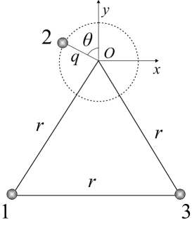
Figure 1: The geometry of the X₃ system as one X atom (numbered as 2) is moved on the contour around the intersection point (located at $O$). The nuclear configuration at the intersection point is an equilateral triangle with $C_{3v}$ symmetry, corresponding to the degeneracy of the ground state and the first excited state.

In Table 1 we list the $x$, $y$, and $z$ components of second-order NAC in two typical Jahn-Teller systems: The prototype H₃ molecule Abrol et al. (2001); Halász et al. (2002); Halaśz et al. (2003) and an alkali-metal trimer Li₃. Martins et al. (1983); Gerber and Schumacher (1978) The three atoms are located in the geometry of Fig. 1 in which one atom is moved on the contour around the intersection point. The contour radius $q$ is chosen as 0.02 bohr, which is sufficiently small so as to be comparable to the condition of the Jahn-Teller model. It is clearly seen that at such a small $q$ the $x$ and $y$ components of second-order NAC in H₃ and Li₃ are significantly large: The nonzero values are in the order of 1000 bohr^-2, which are much larger than those of first-order NAC (which are in the order of $1/q$). In the meanwhile, both the magnitude and relative signs of TDDFT results are in good agreement with the Jahn-Teller model. (The ideal values of second-order NAC from the Jahn-Teller model can be derived from the derivatives of the first-order NAC, as shown by Appendix A.) On the other hand, it is noted that the $z$ components of second-order NAC are quite small but nonzero, either in H₃ or Li₃. This is different from the zero values of $z$ components of first-order NAC in X₃ systems near intersection points. The Jahn-Teller model predicts that the $x$ and $y$ components of second-order NAC only depend on contour radius $q$ and angle $\theta$, while there is an additional dependence of $z$ component on the internuclear distance $r$. In our calculations we set $r_{\mathrm{H-H}}$ = 1.9729 bohr and $r_{\mathrm{Li-Li}}$ = 5.0 bohr respectively, therefore, TDDFT calculations are expected to give different $z$ components for H₃ and Li₃, and the results seem to give such a difference: Both the magnitude and sign agree with the ideal values corresponding to the above internuclear distances. However, since the $z$ components are quite small we need to make sure whether they are intrinsically nonzero. For this purpose we have made a detailed examination of the $z$ components of second-order NAC on the three atoms of H₃ as a function of the contour angle $\theta$, as shown by Fig. 2. As $\theta$ is varied from 0 to 180^∘, the $z$ components on all atoms, although small, show clear dependences on $\theta$ and agree well with the Jahn-Teller model. This means that the small $z$ components of second-order NAC are intrinsically nonzero and have been accurately reproduced by TDDFT.

Table 1: The calculated $x$, $y$ and $z$ components of second-order NAC (in bohr^-2) on three atoms of H₃ and Li₃, which are at the geometry of Fig. 1. The contour radius $q$ is 0.02 bohr and angle $\theta$ is 0. The ideal values from the Jahn-Teller model, as derived in Appendix A and summarized in Table 5, are also listed for comparison. It is noted that the $z$ components of second-order NAC in the Jahn-Teller model are dependent on atomic distances and have been derived within two sets of parameters: the values inside the parenthesis are derived by $r_{\text{Li-Li}}$ = 5.0 bohr, while the others outside are derived by $r_{\text{H-H}}$ = 1.9729 bohr.

		$x\quad$	$y\quad$	$z\quad$
H3	atom 1	1085.88	-1074.36	12.75
	atom 2	0.30	0.00	0.00
	atom 3	-1085.30	1073.36	-12.68
Li3	atom 1	1102.08	-1090.50	4.37
	atom 2	1.44	0.00	0.00
	atom 3	-1099.12	1086.05	-4.71
Model	atom 1	1082.53	-1082.53	12.67 (5.0)
	atom 2	0.00	0.00	0.0 (0.0)
	atom 3	-1082.53	1082.53	-12.67 (-5.0)

Another point noteworthy in Table 1 is the sum of $x$, $y$ and $z$ components. In contrary to the vector form of first-order NAC, second-order NAC are scalars due to the presence of the scalar Laplacian, therefore, only the sum of $x$, $y$ and $z$ components are meaningful in the nonadiabatic dynamics simulation. Table 1 shows the sum of components in both H₃ and Li₃ are small, as predicted by the Jahn-Teller model. This can provide the background for the the neglect of second-order NAC in practical simulations. Martínez (1997); Martínez et al. (1997); Ben-Nun and Martínez (1998)

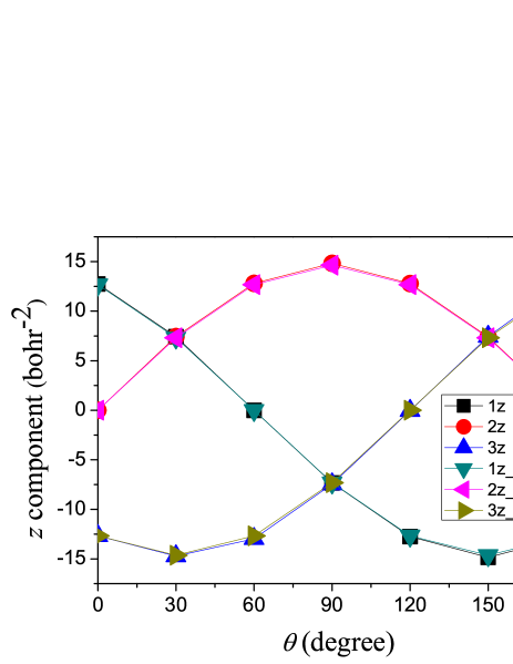
Figure 2: The $z$ components of second-order NAC on the three atoms of H₃. The labels 1z, 2z and 3z denote the $z$ components on atom 1, 2 and 3, while 1z_JT, 2z_JT and 3z_JT denote those from the Jahn-Teller model, respectively.

IV.2 Renner-Teller systems

In Table 2 we list the $x$, $y$, and $z$ components of second-order NAC in several typical Renner-Teller systems: The BH₂, CH${}_{2}^{+}$, NH₂ and H₂O⁺ molecules, Liu et al. (2010); Halász et al. (2006) which are in the geometry of Fig. 3 with the contour angle $\theta$ = 0. The contour radius $q$ is chosen as 0.1 bohr, which is known to be sufficiently small and can be comparable to the condition of the Renner-Teller model. The internuclear distances are set as $r_{\mathrm{H-B}}$ = 2.0 bohr, $r_{\mathrm{H-C}}$ = 2.0 bohr, $r_{\mathrm{H-N}}$ = 1.95 bohr, and $r_{\mathrm{H-O}}$ = 1.85 bohr. It is interesting to see that all components of second-order NAC on three atoms of all molecules are negligibly small (reminding that the first-order NAC in Renner-Teller systems are in the order of $1/q$) and agree with the Renner-Teller model. (The ideal values of second-order NAC from the Renner-Teller model can be derived from the derivatives of the first-order NAC, as shown by Appendix B.) As a matter of fact, NAC of Renner-Teller system do not dependent on the contour angle $\theta$, and thus the negligibly small values of second-order NAC in demonstrated systems are not accidental results for a specified geometry, but indicate that they are intrinsically zero. In connection with the nonadiabatic dynamics simulation, it is thus verified that the sum of $x$, $y$ and $z$ components can be regarded as zero in Renner-Teller systems. This also provides a background for the the neglect of second-order NAC in practical dynamics simulations. Martínez (1997); Martínez et al. (1997); Ben-Nun and Martínez (1998)

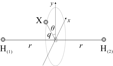
Figure 3: Geometry of the XH₂ or XH${}_{2}^{+}$ system when the X atom is moved on the contour around the Renner-Teller intersection point (indicated by the open square) on the collinear axis. The contour, with radius $q$ and angle $\theta$, is fixed in the $xy$ plane, which is perpendicular to the HH axis. The two hydrogen atoms are set to be symmetric to the plane.

Table 2: The calculated $x$, $y$ and $z$ components of second-order NAC (in bohr^-2) on three atoms of BH₂, CH${}_{2}^{+}$, NH₂ and H₂O⁺, which are at the geometry of Fig. 3. The contour radius $q$ is 0.1 bohr and the angle $\theta$ is 0. The ideal values from the Renner-Teller model, as derived in Appendix B, are also listed for comparison.

		$x\quad$	$y\quad$	$z\quad$
BH2	atom H(1)	0.015	0.0	0.0
	atom B	0.016	0.0	0.0
	atom H(2)	0.015	0.0	0.0
CH${}_{2}^{+}$	atom H(1)	-0.012	0.0	0.0
	atom C	0.013	0.0	0.0
	atom H(2)	-0.012	0.0	0.0
NH2	atom H(1)	0.018	0.0	0.0
	atom N	0.018	0.0	0.0
	atom H(2)	0.018	0.0	0.0
H2O+	atom H(1)	-0.0035	0.0	0.0
	atom O	0.021	0.0	0.0
	atom H(2)	0.0014	0.0	0.0
Model	atom 1	0.0	0.0	0.0
	atom 2	0.0	0.0	0.0
	atom 3	0.0	0.0	0.0

IV.3 Elliptic Jahn-Teller system

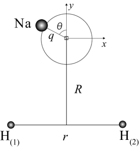
Figure 4: The geometry of the NaH₂ system as the Na atom is moved on the contour around the conical intersection point (indicated by the open square). The nuclear configuration at the conical intersection point is an isoseles triangle with C_2v symmetry.

Table 3: Calculated values of $x$, $y$ and $z$ components of second-order NAC (in bohr^-2) on the three atoms of NaH₂, which are in the geometry shown by Fig. 4 with the contour radius $q$=0.1 bohr and angle $\theta$ = 60^∘.

	$x$	$y$	$z$
atom Na	20.54	-110.13	1.23
atom H(1)	-542.53	-10.94	-2.89
atom H(2)	-618.23	51.59	-5.42

In Table 3 we list TDDFT calculation results of the $x$, $y$, and $z$ components of second-order NAC on the three atoms of NaH₂, which is known as an elliptic Jahn-Teller system.Yarkony (1986); Vibók et al. (2003) The three atoms are located in the geometry of Fig. 4 with the contour angle $\theta$ = 60^∘. Other parameters regarding the geometry are $r$ = 2.18 bohr and $R$ = 3.6127 bohr, according to the intersection point determined in our previous work.Hu et al. (2008) For an elliptic Jahn-Teller systems, the angular NAC $A_{\theta}$ is not just in a quantized value of 0.5, but shows a strong dependence on the contour angle $\theta$. Using the similar procedures in Appendix A but setting the angular NAC, $A_{\theta}$, as a variable rather than a constant of 0.5, we can easily get the conclusion that second-order NAC would depend on $\frac{\partial A_{\theta}}{\partial\theta}$, i.e., the slope of angular NAC with respect to $\theta$. Therefore, we set $\theta$ as 60^∘ at which $\frac{\partial A_{\theta}}{\partial\theta}$ is relatively large, as revealed by our previous work.Hu et al. (2008) It is clearly seen that under such a condition the magnitudes of $x$ and $y$ components become unbalanced in comparison with the Jahn-Teller systems. Meanwhile, the $z$ components are still relatively small. Therefore, the sum of $x$, $y$ and $z$ components of second-order NAC can not be negligibly small. Regarding the role of NAC in the nonadiabatic dynamics simulation, it is thus suggested to include second-order NAC in the rigorous simulation of general molecular systems, which might possess accidental conical intersections without any symmetry requirements as in Jahn-Teller systems.

V Conclusion

We have proposed an efficient TDDFT method for calculating second-order NAC between ground state and singly excited states, which is based on the Casida ansatz adapted for first-order NAC, while the calculation procedure can be done without the need of explicitly constructing auxiliary excited-state wavefunctions. Our formulation can be justified when the TDA is valid. Within the modified linear response theory, the TDDFT formulation is reduced to the Slater transition method in doublet systems. Test calculations are carried out in the immediate vicinity of various types of intersection points. The results are in good agreement with the ideal values derived from Jahn-Teller or Renner-Teller models. Contrary to the diverging behavior of first-order NAC near intersections, the Cartesian components of second-order NAC are shown to be negligibly small near Renner-Teller intersections, while they are significantly large near Jahn-Teller intersections. Nevertheless, the Cartesian components of second-order NAC can cancel each other to a large extent in Jahn-Teller systems, showing the background of neglecting second-order NAC in nonadiabatic dynamics simulations. On the other hand, it is revealed that such a cancellation becomes less effective in an elliptic Jahn-Teller system and thus the role of second-order NAC needs to be evaluated in the rigorous framework. Finally, it is noted that the performance of TDDFT on the computation of second-order NAC needs to be further validated, particularly for a general atomic geometry, which requires reference data and remains future work.

Appendix A Second-order NAC from the Jahn-Teller model

The Jahn-Teller model describes a class of systems in which a set of nuclear coordinates are coupled to a two-level system consisting of the ground state and the first excited state of appropriate symmetry Desouter-Lecomte et al. (1985). Figure 5 shows an arbitrary configuration of a Jahn-Teller trimer. When the contour radius $q$ is sufficiently small, the angular NAC has a quantized value of $\frac{1}{2}$ according to the Jahn-Teller model. Desouter-Lecomte et al. (1985) All components of first-order NAC on the three atoms can thus be uniquely determined, as shown by Table 4.

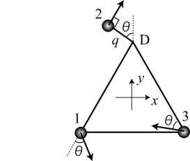
Figure 5: Configuration of a Jahn-Teller trimer in the $xy$ plane, in which atom 2 is regarded on a contour with radius $q$ and angle $\theta$ around the intersection point (vertex D of the equilateral triangle). Arrows represent NAC vectors on the three atoms.

Table 4: The $x$, $y$ and $z$ components of first-order NAC on the three atoms of a Jahn-Teller trimer, which are in the geometry shown by Fig. 5. $q$ is the contour radius and $\theta$ is the contour angle.

	$x$	$y$	$z$
atom 1	$\frac{0.5}{q}\cos(120^{\circ}-\theta)$	$-\frac{0.5}{q}\sin(120^{\circ}-\theta)$	0
atom 2	$\frac{0.5}{q}\cos\theta$	$\frac{0.5}{q}\sin\theta$	0
atom 3	$-\frac{0.5}{q}\cos(60^{\circ}-\theta)$	$\frac{0.5}{q}\sin(60^{\circ}-\theta)$	0

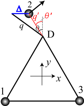
Figure 6: Schematic view of the derivation process of the $x$ component of second-order NAC on atom 2. A small displacement $\Delta$ is made in the $x$ direction for atom 2. After displacement the contour radius is changed from $q$ to $q^{\prime}$, and the contour angle is from $\theta$ to $\theta^{\prime}$. The arrow denotes the new NAC vector on atom 2.

To derive the $x$ component of second-order NAC on atom 2, we move atom 2 in the $x$ direction with a small displacement $\Delta$, as shown by Fig. 6. Since the Jahn-Teller model is a two-level system, we can get

$$\left\langle\Psi_{0}\right|\frac{\partial^{2}}{\partial x_{2}^{2}}\left|\Psi_{1}\right\rangle=\frac{\partial}{\partial x_{2}}\left\langle\Psi_{0}\right|\frac{\partial}{\partial x_{2}}\left|\Psi_{1}\right\rangle=\frac{A_{x_{2}}^{\mathrm{disp}}-A_{x_{2}}}{\Delta},$$ (36)

where $A_{x_{2}}$ is the $x$ component of first-order NAC before the displacement, as listed in Table 4. The new $x$ component of first-order NAC on atom 2 after the displacement, $A_{x_{2}}^{\text{disp}}$, can be determined from the new geometry as

$$A_{x_{2}}^{\text{disp}}=\frac{0.5}{q^{\prime}}\cos\theta^{\prime},$$ (37)

where

$$q^{\prime}=\sqrt{q^{2}\cos^{2}\theta+(q\sin\theta-\Delta)^{2}}$$ (38)

and

$$\theta^{\prime}=\arccos\left(\frac{q\cos\theta}{q^{\prime}}\right).$$ (39)

By taking $\Delta\to 0$ in Eq. (36), we can get

$$\left\langle\Psi_{0}\right|\frac{\partial^{2}}{\partial x_{2}^{2}}\left|\Psi_{1}\right\rangle=\lim_{\Delta\to 0}\frac{1}{\Delta}\left(\frac{0.5}{q^{\prime}}\cos\theta^{\prime}-\frac{0.5}{q}\cos\theta\right)=\frac{0.5}{q^{2}}\sin 2\theta$$ (40)

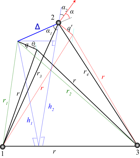
Figure 7: Schematic view of the derivation process of the $z$ component of 2nd-order NAC on atom 2. After a small displacement $\Delta$ is made in the $z$ direction for atom 2, the contour radius is changed from $q$ to $q^{\prime}$, and the NAC vector (denoted by the arrow ending on atom 2) is located in the new atomic plane.

The derivation of the $y$ component of second-order NAC on atom 2 is similar to that of the $x$ component in the above, thus the detail is not shown here. Next, to derive the $z$ component, we move atom 2 in the $z$ direction as shown by Fig. 7, and then we can get

$$\left\langle\Psi_{0}\right|\frac{\partial^{2}}{\partial z_{2}^{2}}\left|\Psi_{1}\right\rangle=\frac{\partial}{\partial z_{2}}\left\langle\Psi_{0}\right|\frac{\partial}{\partial z_{2}}\left|\Psi_{1}\right\rangle=\frac{A_{z_{2}}^{\mathrm{disp}}}{\Delta},$$ (41)

which uses the fact that the $z$ component of first-order NAC on atom 2 before the displacement is zero. The new geometry after the displacement gives

$$A_{z_{2}}^{\text{disp}}=\frac{0.5}{q^{\prime}}\cos\alpha=\frac{0.5}{q^{\prime}}\cos\alpha_{1}\cos\alpha_{2},$$ (42)

where $q^{\prime}$ is the new contour radius around the vertex of the equilateral triangle in the new atomic plane. $\alpha$ is the angle between the new NAC vector and the $z$ axis, $\alpha_{1}$ is the angle between the new atomic plane and the $z$ axis, and $\alpha_{2}$ is the angle between the new NAC vector and the projection of the $z$ axis in the new atomic plane. Using the geometric relationships shown by Fig. 7, we can get

$$q^{\prime}=\sqrt{r_{3}^{2}+r^{2}-2r_{3}r\cos\left[\arccos\left(\frac{r_{3}^{2}+r^{2}-r_{4}^{2}}{2r_{3}r}\right)-60^{\circ}\right]},$$ (43)

$$\alpha_{1}=\arcsin\left(\frac{h_{1}}{h_{2}}\right),$$ (44)

and

$$\alpha_{2}=90^{\circ}-\arccos\left(\frac{q^{\prime 2}+r_{4}^{2}-r^{2}}{2q^{\prime}r_{4}}\right)-\arccos\left(\frac{h_{2}}{r_{4}}\right).$$ (45)

The auxiliary quantities in the above equations are calculated as

$$r_{3}=\sqrt{r_{1}^{2}+\Delta^{2}},r_{4}=\sqrt{r_{2}^{2}+\Delta^{2}},$$

$$h_{1}=\frac{\sqrt{3}}{2}+q\cos\theta,h_{2}=\sqrt{h_{1}^{2}+\Delta^{2}},$$

$$r_{1}=\sqrt{r^{2}+q^{2}-2qr\cos(150^{\circ}-\theta)},$$

$$r_{2}=\sqrt{r^{2}+q^{2}-2qr\cos(210^{\circ}-\theta)}.$$

By taking $\Delta\to 0$, we can get $r_{3}\to r_{1}$, $r_{4}\to r_{2}$, $h_{2}\to h_{1}$, $q^{\prime}\to q$, and $\alpha_{2}\to 90^{\circ}-\theta$. Then Eq. (41) is reduced to

$$\left\langle\Psi_{0}\right|\frac{\partial^{2}}{\partial z_{2}^{2}}\left|\Psi_{1}\right\rangle=\lim_{\Delta\to 0}\frac{1}{\Delta}\frac{0.5}{q}\cos\left[\arcsin\left(\frac{h_{1}}{h_{2}}\right)\right]\cos(90^{\circ}-\theta)=\frac{0.5}{q}\frac{1}{\sqrt{3}r/2}\sin\theta,$$ (46)

where we have used the fact that $r\gg q$.

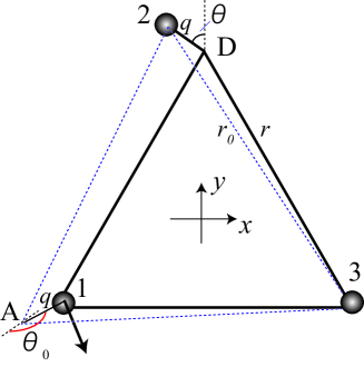
Figure 8: Schematic view of the derivation process of 2nd-order NAC components on atom 1, which is regarded as rotating around vertex A of a new equilateral triangle with side length $r_{0}$. The corresponding contour radius and angle is $q$ and $\theta_{0}$, respectively.

To derive components of second-order NAC on atom 1 and atom 3, we need not make displacements but can merely use the fact that the three atoms are equivalent, i.e., not only atom 2 can be regarded as rotating in a contour around the intersection point, other two atoms can also be taken into such a view. In Fig. 8, where atomic geometry is the same as in Fig. 5, atom 1 is regarded as rotating around the intersection point A with contour radius $q$ and angle $\theta_{0}$. Here A is the vertex of a new equilateral triangle with side length $r_{0}$. The geometric analysis gives

$$r_{0}=\sqrt{q^{2}+r^{2}-2qr\cos(210^{\circ}-\theta)},$$ (47)

and

$$\theta_{0}=150^{\circ}+\arccos\left(\frac{q^{2}+r_{0}^{2}-r^{2}}{2qr_{0}}\right)=150^{\circ}+\arccos\left[\frac{q-r\cos(210^{\circ}-\theta)}{r}\right].$$ (48)

Using the fact that $r\gg q$ we can easily get $r_{0}=r$ and $\theta_{0}=120^{\circ}+\theta$. Replacing $r$ and $\theta$ in the expression of second-order NAC components on atom 2 with $r_{0}$ and $\theta_{0}$, we can immediately get the results for atom 1.

The results for atom 3 can be derived in a way similar to that for atom 1. The final results of second-order NAC components on all atoms are listed in Table 5.

Table 5: The $x$, $y$ and $z$ components of second-order NAC on the three atoms of a Jahn-Teller trimer, which are in the geometry shown by Fig. 5. $q$ is the contour radius and $\theta$ is the contour angle.

	$x$	$y$	$z$
atom 1	$\frac{0.5}{q^{2}}\cos(30^{\circ}+2\theta)$	$-\frac{0.5}{q^{2}}\cos(30^{\circ}+2\theta)$	$\frac{0.5}{q}\frac{1}{\sqrt{3}r/2}\sin(\theta+120^{\circ})$
atom 2	$\frac{0.5}{q^{2}}\sin 2\theta$	$-\frac{0.5}{q^{2}}\sin 2\theta$	$\frac{0.5}{q}\frac{1}{\sqrt{3}r/2}\sin\theta$
atom 3	$-\frac{0.5}{q^{2}}\sin(120^{\circ}-2\theta)$	$\frac{0.5}{q^{2}}\sin(120^{\circ}-2\theta)$	$\frac{0.5}{q}\frac{1}{\sqrt{3}r/2}\sin(\theta-120^{\circ})$

Appendix B Second-order NAC from the Renner-Teller model

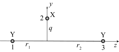
Figure 9: Configuration of an XY₂ Renner-Teller system in the $yz$ plane. The three atoms are located in a geometry slightly distorted from the linear geometry, and atom 2 is regarded on a contour around the $z$ axis with contour radius $q$.

Table 6: The $x$, $y$ and $z$ components of first-order NAC on the three atoms of an XY₂ Renner-Teller system, which is in the geometry shown by Fig. 9. $q$ is the contour radius, while $r_{1}$ ($r_{2}$) is the distance of atom 1 (atom 3) from the intersection point.

	$x$	$y$	$z$
atom 1	$-\frac{1}{q}\frac{r_{2}}{r_{1}+r_{2}}$	0	0
atom 2	$\frac{1}{q}$	0	0
atom 3	$-\frac{1}{q}\frac{r_{1}}{r_{1}+r_{2}}$	0	0

Figure 9 shows an arbitrary configuration of an XY₂ Reller-Teller systems, where the X atom is moved with a sufficiently small displacement $q$ from the $z$ axis, which is the seam of Renner-Teller intersections. According to the Renner-Teller model Desouter-Lecomte et al. (1985), the angular NAC has a quantized value of 1.0 and all components of first-order NAC on three atoms can be determined, as shown by Table 6. Note that all $y$ and $z$ components are equal to zero, meaning that the NAC vectors are parallel to the $x$ axis.

Because the first-order NAC vectors are perpendicular to the $yz$ plane, small movement of atoms in the $yz$ plane will not alter the direction of NAC vectors and the $y$ and $z$ components of first-order NAC are kept to be zero after the displacement. Therefore, we can immediately conclude that $y$ and $z$ components of second-order NAC on all atoms are zero.

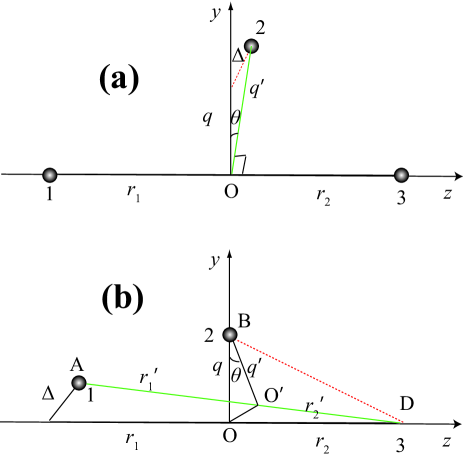
Figure 10: Schematic view of the derivation process of the $x$ component of second-order NAC on (a) atom 2 and (b) atom 1. A small displacement $\Delta$ is made in the $x$ direction for atom 2 in (a) and atom 1 in (b). After displacement the contour radius is changed from $q$ to $q^{\prime}$. Note that in (b) the intersection point is changed from O to $\text{O}^{\prime}$.

To derive the $x$ component of second-order NAC on atom 2, we move atom 2 in the $x$ direction, as shown by Fig. 10(a). Since the Renner-Teller model is a two-level system, we can get

$$\left\langle\Psi_{0}\right|\frac{\partial^{2}}{\partial x_{2}^{2}}\left|\Psi_{1}\right\rangle=\frac{\partial}{\partial x_{2}}\left\langle\Psi_{0}\right|\frac{\partial}{\partial x_{2}}\left|\Psi_{1}\right\rangle=\frac{A_{x_{2}}^{\mathrm{disp}}-A_{x_{2}}}{\Delta},$$ (49)

where

$$A_{x_{2}}=\frac{1}{q}.$$ (50)

The new geometry after the displacement gives

$$A_{x_{2}}^{\text{disp}}=\frac{1}{q^{\prime}}\cos\theta,$$ (51)

where $q^{\prime}=\sqrt{q^{2}+\Delta^{2}}$ and $\theta=\arccos(q/q^{\prime})$. By taking $\Delta\to 0$ in Eq. (49), we can get

$$\left\langle\Psi_{0}\right|\frac{\partial^{2}}{\partial x_{2}^{2}}\left|\Psi_{1}\right\rangle=\lim_{\Delta\to 0}\frac{1}{\Delta}\left[\frac{-\Delta^{2}}{(q^{2}+\Delta^{2})q}\right]=0.$$ (52)

In a similar way the $x$ component of second-order NAC on atom 1 can be derived by displacing atom $1$ in the $x$ direction, shown by Fig. 10(b), as

$$\left\langle\Psi_{0}\right|\frac{\partial^{2}}{\partial x_{1}^{2}}\left|\Psi_{1}\right\rangle=\frac{\partial}{\partial x_{1}}\left\langle\Psi_{0}\right|\frac{\partial}{\partial x_{1}}\left|\Psi_{1}\right\rangle=\frac{A_{x_{1}}^{\mathrm{disp}}-A_{x_{1}}}{\Delta},$$ (53)

where

$$A_{x_{1}}=-\frac{1}{q}\frac{r_{2}}{r_{1}+r_{2}},$$ (54)

$$A_{x_{1}}^{\text{disp}}=-\frac{1}{q^{\prime}}\frac{r_{2}^{\prime}}{r_{1}^{\prime}+r_{2}^{\prime}}\cos\theta,$$ (55)

$$q^{\prime}=\sqrt{q^{2}+(r_{2}-r_{2}^{\prime})^{2}},$$ (56)

$$\theta=\arccos(q/q^{\prime}),$$ (57)

$$r_{2}^{\prime}=r_{2}\cdot\frac{r_{1}+r_{2}}{r_{1}^{\prime}+r_{2}^{\prime}}=r_{2}\cdot\frac{r_{1}+r_{2}}{\sqrt{(r_{1}+r_{2})^{2}+\Delta^{2}}}.$$ (58)

Taking $\Delta\to 0$ in Eq. (53), we can get

$$\left\langle\Psi_{0}\right|\frac{\partial^{2}}{\partial x_{1}^{2}}\left|\Psi_{1}\right\rangle=\lim_{\Delta\to 0}\frac{1}{\Delta}\frac{q^{2}r_{2}\Delta^{2}+r_{2}^{3}\Delta^{2}}{\left[q^{2}\Delta^{2}+q^{2}(r_{1}+r_{2})^{2}+r_{2}^{2}\Delta^{2})\right]q(r_{1}+r_{2})}=0.$$ (59)

Finally, since the derivation of $x$ component of second-order NAC on atom 3 is essentially equivalent to that of atom 1, the result for atom 3 is also 0.

In one word, all components of second-order NAC on the three atoms of the Renner-Teller system are equal to zero.

References

- Yarkony (1996) D. R. Yarkony, Rev. Mod. Phys. 68, 985 (1996).
- Nakamura (2002) H. Nakamura, Nonadiabatic Transitions: Concepts, Basic Theories,and Applications (World Scientific, Singapore, 2002).
- Baer (2006) M. Baer, Beyond Born-Oppenheimer: Electronic Nonadiabatic Coupling Terms and Conical Intersections (Wiley, Hoboken, New Jersey, 2006).
- Doltsinis and Marx (2002) N. L. Doltsinis and D. Marx, Phys. Rev. Lett. 88, 166402 (2002).
- Li et al. (2005) X. Li, J. C. Tully, H. B. Schlegel, and M. J. Frisch, J. Chem. Phys. 123, 084106 (2005).
- Isborn et al. (2007) C. M. Isborn, X. Li, and J. C. Tully, J. Chem. Phys. 126, 134307 (2007).
- Martínez (1997) T. D. Martínez, Chem. Phys. Lett. 272, 139 (1997).
- Yonehara and Takatsuka (2008a) T. Yonehara and K. Takatsuka, J. Chem. Phys. 128, 154104 (2008a).
- Yonehara and Takatsuka (2008b) T. Yonehara and K. Takatsuka, J. Chem. Phys. 129, 134109 (2008b).
- Billeter and Curioni (2005) S. R. Billeter and A. Curioni, J. Chem. Phys. 122, 034105 (2005).
- Chernyak and Mukamel (2000) V. Chernyak and S. Mukamel, J. Chem. Phys. 112, 3572 (2000).
- Baer (2002) R. Baer, Chem. Phys. Lett. 364, 75 (2002).
- Hu et al. (2007) C. Hu, H. Hirai, and O. Sugino, J. Chem. Phys. 127, 064103 (2007).
- Hu et al. (2008) C. Hu, H. Hirai, and O. Sugino, J. Chem. Phys. 128, 154111 (2008).
- (15) M. E. Casida, in Recent Advances in Density Functional Methods, Part I, edited by D. P. Chong (World Scientific, Singapore, 1995), p. 155.
- Jamorski et al. (1996) C. Jamorski, M. E. Casida, and D. R. Salahub, J. Chem. Phys. 104, 5134 (1996).
- Hu et al. (2009) C. Hu, O. Sugino, and Y. Tateyama, J. Chem. Phys. 131, 114101 (2009).
- Send and Furche (2010) R. Send and F. Furche, J. Chem. Phys. 132, 044107 (2010).
- Tapavicza et al. (2007) E. Tapavicza, I. Tavernelli, and U. Rothlisberger, Phys. Rev. Lett. 98, 023001 (2007).
- Tavernelli et al. (2009a) I. Tavernelli, E. Tapavicza, and U. Rothlisberger, J. Chem. Phys. 130, 124107 (2009a).
- Tavernelli et al. (2010a) I. Tavernelli, B. F. E. Curchod, A. Laktionov, and U. Rothlisberger, J. Chem. Phys 133, 194104 (2010a).
- Hu et al. (2010) C. Hu, O. Sugino, H. Hirai, and Y. Tateyama, Phys. Rev. A 82, 062508 (2010).
- Tavernelli et al. (2009b) I. Tavernelli, B. F. E. Curchod, and U. Rothlisberger, J. Chem. Phys. 131, 196101 (2009b).
- Tavernelli et al. (2010b) I. Tavernelli, B. F. E. Curchod, and U. Rothlisberger, Phys. Rev. A 81, 052508 (2010b).
- Tapavicza et al. (2008) E. Tapavicza, I. Tavernelli, U. Rothlisberger, C. Filippi, and M. E. Casida, J. Chem. Phys. 129, 124108 (2008).
- Werner et al. (2008) U. Werner, R. Mitrić, T. Suzuki, and V. Bonačić-Koutecký, Chem. Phys. 349, 319 (2008).
- Hirai and Sugino (2009) H. Hirai and O. Sugino, Phys. Chem. Chem. Phys. 11, 4570 (2009).
- Redmon (1982) L. T. Redmon, Phys. Rev. A 25, 2453 (1982).
- Lengsfield III et al. (1986) B. H. Lengsfield III, , and D. R. Yarkony, J. Chem. Phys. 84, 348 (1986).
- Ågren et al. (1986) H. Ågren, A. Flores-Riveros, and H. J. A. Jensen, Phys. Rev. A 34, 4606 (1986).
- Santer et al. (2001) M. Santer, U. Manthe, and G. Stock, J. Chem. Phys. 114, 2001 (2001).
- Martínez et al. (1997) T. J. Martínez, M. Ben-Nun, and R. D. Levine, J. Phys. Chem. A 101, 6389 (1997).
- Ben-Nun and Martínez (1998) M. Ben-Nun and T. J. Martínez, Chem. Phys. Lett. 298, 57 (1998).
- Hu et al. (2006) C. Hu, O. Sugino, and Y. Miyamoto, Phys. Rev. A 74, 032508 (2006).
- Hu and Sugino (2007) C. Hu and O. Sugino, J. Chem. Phys. 126, 074112 (2007).
- Bersuker (2001) I. B. Bersuker, Chem. Rev. 101, 1067 (2001).
- Bersuker (2006) I. B. Bersuker, The Jahn-Teller Effect (Cambridge Univ. Press, Cambridge, 2006).
- Jungen and Merer (1980) C. Jungen and A. J. Merer, Mol. Phys. 40, 1 (1980).
- Mikhailov et al. (2006) I. A. Mikhailov, V. Kokoouline, Å. Larson, S. Tonzani, and C. H. Greene, Phys. Rev. A 74, 032707 (2006).
- Vibók et al. (2003) Á. Vibók, G. J. Halász, T. Vèrteśi, S. Suhai, M. Baer, and J. P. Toennies, J. Chem. Phys. 119, 6588 (2003).
- (41) X. Gonze, J.-M. Beuken, R. Caracas, F. Detraux, M. Fuchs, G.-M. Rignanese, L. Sindic, M. Verstraete, G. Zerah, F. Jollet, M. Torrent, A. Roy, M. Mikami, Ph. Ghosez, J.-Y. Raty, and D. C. Allan, Comp. Mater. Sci. 25, 478 (2002). The ABINIT code is a common project of the Université Catholique de Louvain, Corning Incorporated, the Université de Liège, Mitsubishi Chemical Corp., and other contributors (URL http://www.abinit.org).
- Goedecker et al. (1996) S. Goedecker, M. Teter, and J. Hutter, Phys. Rev. B. 54, 1703 (1996).
- Troullier and Martins (1991) N. Troullier and J. L. Martins, Phys. Rev. B 43, 1993 (1991).
- Louie et al. (1982) S. G. Louie, S. Froyen, and M. L. Cohen, Phys. Rev. B 26, 1738 (1982).
- Abrol et al. (2001) R. Abrol, A. Shaw, and A. Kuppermann, J. Chem. Phys. 115, 4640 (2001).
- Halász et al. (2002) G. Halász, Á. Vibók, A. M. Mebel, and M. Baer, Chem. Phys. Lett. 358, 163 (2002).
- Halaśz et al. (2003) G. Halaśz, Á. Vibók, A. M. Mebel, and M. Baer, J. Chem. Phys. 118, 3052 (2003).
- Martins et al. (1983) J. L. Martins, R. Car, and J. Buttet, J. Chem. Phys. 78, 5646 (1983).
- Gerber and Schumacher (1978) W. H. Gerber and E. Schumacher, J. Chem. Phys. 69, 1692 (1978).
- Liu et al. (2010) Y. Liu, I. B. Bersuker, W. Zou, and J. E. Boggs, Chem. Phys. 376, 30 (2010).
- Halász et al. (2006) G. J. Halász, Á. Vibók, R. Baer, and M. Baer, J. Chem. Phys. 124, 081106 (2006).
- Yarkony (1986) D. R. Yarkony, J. Chem. Phys. 84, 3206 (1986).
- Desouter-Lecomte et al. (1985) M. Desouter-Lecomte, D. Dehareng, B. Leyh-Nihant, M. Th. Praet, A. J. Lorquet, and J. C. Lorquet, J. Phys. Chem. 89, 214 (1985).