How Many Transmit Antennas to Use in a MIMO Interference Channel

Abstract

The problem of finding the optimal number of data streams to transmit in a multi-user MIMO scenario, where both the transmitters and receivers are equipped with multiple antennas is considered. Without channel state information at any transmitter, with a zero-forcing receiver each user is shown to transmit a single data stream to maximize its own outage capacity in the presence of sufficient number of users. Transmitting a single data stream is also shown to be optimal in terms of maximizing the sum of the outage capacities in the presence of sufficient number of users.

I Introduction

Employing multiple antennas at transmitters and receivers is well known to improve the performance of wireless communication by either decreasing the bit-error rate (BER) [1], or increasing the channel capacity [2, 3]. A key assumption used in [1, 2, 3] is that the transmission is interference free, i.e. each multiple antenna equipped receiver only receives signal from its corresponding multi-antenna transmitter, and no other transmitter is transmitting at the same time. This assumption is easy to justify in practice with base-station based centralized controllers, however, it fails to work in decentralized wireless network setting such as sensor networks, ad-hoc networks etc., where there are large number of uncoordinated transmitters. In a decentralized wireless network, each node transmits independently, thereby possibly causing interference to all the other nodes.

We consider a decentralized wireless network setting, where there are $N$ non-cooperating transmitter-receiver pairs or links, and all the transmitter and receiver nodes are equipped with $M$ antennas (popularly known as the MIMO interference channel). We assume that no transmitter has any channel state information (CSI), while each receiver has CSI only for the channel from its corresponding transmitter. With its CSI, we assume that each receiver uses a zero-forcing ZF receiver to decode the different streams sent from its corresponding transmitter. The ZF receiver is considered because of its low complexity implementation. Our results can be generalized to MMSE receivers as well. With ZF, we consider outage capacity as the performance metric owing to its analytical tractability and practical significance. Outage capacity is defined as the rate of transmission multiplied with the probability that the transmission is not in outage [2], where outage is defined as the event that the mutual information of the channel is less than the target rate of transmission. In this paper we are interested in finding the optimal number of data streams to send from each transmitter that maximizes the sum outage capacity of the MIMO interference channel with ZF.

I-A Contributions

The contributions of this paper are as follows

• We show that with sufficiently large number of users $N$, to maximize the individual outage capacity it is optimal for each user to transmit a single data stream irrespective of the number of data streams transmitted by other users.

• For sufficiently large number of users $N$, we show that the sum outage capacity is maximized when each user transmits a single data stream.

I-B Comparison with prior work

When no transmitter has any CSI, under an average power constraint, Shannon capacity is equal to the expected mutual information that is obtained using the maximum likelihood (ML) decoding. ML decoding, however, is quite complicated in a multi-user MIMO scenario, and finding the optimal number of data streams to transmit that maximize the mutual information with ML decoding is quite challenging. Thus, for analytical tractability and to get insights into the problem, we consider a simple ZF decoder [4], and use outage capacity as the performance metric. Outage framework has been extensively used in past to understand the performance of multiple antenna systems [2, 5, 6]. In this paper we show that transmitting a single data stream is selfishly optimal for each user to maximize its own outage capacity in the presence of sufficient number of transmitter-receiver pairs.

Without any CSI at the transmitter, finding the optimal number of data streams that maximize the sum capacity has attracted a lot of attention [7, 8, 6]. For a large ad-hoc network, where the transmitter locations are distributed as a Poisson point process, the optimal number of data streams to transmit that maximize the transmission capacity [9] has been derived in [6, 8] for $M,N\rightarrow\infty$. When each receiver employs interference cancelation, single data stream transmission has been shown to be optimal [6], while without interference cancelation, using the number of data streams equal to a fraction of the total transmit antennas [6, 8] has been shown to maximize the transmission capacity. Single data stream transmission has also been shown to maximize the sum of the ergodic Shannon capacities [7] for the limiting case of extremely large interference power. Unlike previous works [8, 6], we consider the finite $N,M$ regime, and do not make any assumptions on the location of transmitters/receivers or the interference power at any receiver in contrast to [7]. Without any of the mentioned assumptions, for an arbitrary MIMO interference channel, in this paper we show that if the number of links $N$ is large enough (typically $\approx M$ when the SIR threshold required for correct decoding is greater than $1$, where $M$ is the number of antennas at each node), then transmitting a single data stream from each user is optimal for maximizing the sum outage capacity.

Notation: Let ${{\mathbf{A}}}$ denote a matrix, ${\bf a}$ a vector and $a_{i}$ the $i^{th}$ element of ${\bf a}$. Transpose and conjugate transpose is denoted by ^T, and ^∗, respectively. A circularly symmetric complex Gaussian random variable $x$ with zero mean and variance $\sigma^{2}$ is denoted as $x\sim{\cal CN}(0,\sigma^{2})$. A chi-square distributed random variable $y$ with $m$ degrees of freedom is denoted by $y\sim\chi^{2}(m)$. t t We use the symbol $:=$ to define a variable.

II System Model

Consider a MIMO interference channel with $N$ transmitter-receiver pairs, where each transmitter and receiver is equipped with $M$ antennas. We assume that each transmitter is only interested in transmitting to its corresponding receiver and has an average power constraint of $P$. We assume that each receiver knows CSI for its corresponding transmitter, however, no CSI is available at any transmitter. With no CSI, the $n^{th}$ transmitter sends data vector ${\mathbf{x}}_{n}\in{\mathbb{C}}^{k_{n}\times 1}$ consisting of $k_{n}$ data streams, where each data stream is independent and ${\cal CN}(0,1)$ distributed, using its $k_{n}$ antennas by distributing its power uniformly over the $k_{n}$ antennas. With this model the received signal at the $n^{th}$ receiver is

$${\mathbf{y}}_{n}=\sqrt{\frac{P}{k_{n}}}{\mathbf{H}}_{nn}{\mathbf{x}}_{n}+\sum_{m=1,m\neq n}^{N}\sqrt{\frac{P}{k_{m}}}{\mathbf{H}}_{mn}{\mathbf{x}}_{m}+{\mathbf{w}}_{n},$$ (1)

where ${\mathbf{H}}_{mn}\in{\mathbb{C}}^{N\times k_{n}}$ is the channel coefficient matrix between the $m^{th}$ transmitter and the $n^{th}$ receiver whose entries are i.i.d. ${\cal CN}(0,1)$, and ${\mathbf{w}}_{n}$ is the additive white Gaussian noise with zero mean and $\sigma^{2}$ variance. For sufficiently large $N,P,$ this system is interference limited and we drop the AWGN contribution in the sequel.

We assume that each receiver decodes the $k_{n}$ data streams independently using a ZF decoder [4]. Hence to decode the $j^{th}$ stream out of the total $k_{n}$ streams at the $n^{th}$ receiver, the received signal is projected onto the null space of the channel coefficient vectors corresponding to the $[1,2,\ldots,j-1,j+1,\ldots,k_{n}]$ data streams. Thus the $n^{th}$ receiver multiplies ${\mathbf{q}}^{n}_{j}$ to the received signal ${\mathbf{y}}_{n}$ to decode its $j^{th}$ stream, if ${\mathbf{q}}_{j}^{n}\in{\cal N}\left([{\mathbf{H}}_{nn}(1)\ldots{\mathbf{H}}_{nn}(j-1){\mathbf{H}}_{nn}(j+1)\ldots{\mathbf{H}}_{nn}(k_{n})]\right)$, where ${\cal N}\left([P]\right)$ represents the null space of columns of $P$, and ${\mathbf{H}}_{nn}(\ell)$ represents the $\ell^{th}$ column of ${\mathbf{H}}_{nn}$.

From (1), using the ZF decoder, the signal-to-interference ratio (SIR) for the $j^{th}$ stream is

$${\mathsf{SIR}}_{j}^{n}=\frac{\frac{P}{k_{n}}|{\mathbf{q}}_{j}^{n}{\mathbf{H}}_{nn}(j)|^{2}}{\sum_{m=1,m\neq n}^{N}\frac{P}{k_{m}}\sum_{\ell=1}^{k_{m}}|{\mathbf{q}}_{j}^{n}{\mathbf{H}}_{mn}(\ell)|^{2}}.$$ (2)

Note that ${\mathsf{SIR}}_{j}^{n}$ is identically distributed for $j=1,2,\dots,k_{n}$ for a fixed $n$, $n=1,2,\ldots,N$. To simplify the notation let $s_{j}^{n}:=|{\mathbf{q}}_{j}^{n}{\mathbf{H}}_{nn}(j)|^{2}$, and $I_{\ell,m}:=|{\mathbf{q}}_{j}^{n}{\mathbf{H}}_{mn}(\ell)|^{2}$. From [10], $s_{j}^{n}\sim\chi_{2(M-k+1)}^{2}$ and $I_{\ell,m}\sim\chi_{2}^{2},\ \forall\ j,n,\ell,m$. Hence ${\mathsf{SIR}}_{j}^{n}=\frac{\frac{P}{k_{n}}s_{j}^{n}}{\sum_{m=1,m\neq n}^{N}\frac{P}{k_{m}}\sum_{\ell=1}^{k_{m}}I_{\ell,m}}$.

We assume that a fixed rate of $R$ bits/sec/Hz is transmitted on each data stream, and transmission on any data stream is deemed to be successful if the SIR on that data stream is larger than a threshold $\beta$, which is a function of $R$, i.e., the transmission is not in outage. Hence the successful rate (outage capacity) obtained on any data stream is the product of $R$ and the probability that the SIR on that link is larger than $\beta$, $P({\mathsf{SIR}}_{j}^{n}\geq\beta)$. Combining all the $k_{n}$ streams the outage capacity on the $n^{th}$ link is $C_{n}:=k_{n}RP({\mathsf{SIR}}_{j}^{n}\geq\beta)$ bits/sec/Hz. Hence the sum outage capacity of the MIMO interference channel with ZF is $C_{sum}:=\sum_{n=1}^{N}C_{n}$, and we want to find the optimal $k_{1},\dots,k_{n}$ that maximize the sum outage capacity, i.e. $\arg\max_{k_{1},\dots,k_{n}}C_{sum}$.

We first solve $\arg\max_{k_{j}}C_{j},\forall\ j$, and use that to solve $\arg\max_{k_{1},\dots,k_{n}}C_{sum}$ as follows.

Theorem 1

Using ZF decoder at each receiver, for any choice of $k_{1},\dots,k_{j-1},k_{j+1},\dots,k_{n}$, $k_{j}=1$ (transmitting a single data stream from the $j^{th}$ user) maximizes the outage capacity $C_{j}$ of the $j^{th}$ user for sufficiently large $N$ (specified in the proof).

Proof: See Appendix A.  ∎

Remark 1

In Appendix A we show that for $\beta>1$, Theorem 1 holds for $N\geq\theta M$, where $\theta>1$ is a constant. Simulation results indicate that $N\approx M$ is sufficient for Theorem 1 to hold when $\beta>1$. Typically $\beta=2^{R}-1$, where $R$ is the rate of transmission in bits/sec/Hz. Thus, for $R>1$ bits/sec/Hz, $N\approx M$ is sufficient for Theorem 1 to hold. Moreover, in any practical system the number of users is much larger than the number of antennas at each node, hence Theorem 1 is applicable for most practical scenarios.

Next, we use Theorem 1 to solve the general problem $\arg\max_{k_{1},\dots,k_{n}}C_{sum}$.

Corollary 1

Using ZF decoder at each receiver, $k_{n}=1\ \forall\ n$ maximizes the sum capacity $C$, i.e. $(1,1,\ldots,1)=\arg\max_{k_{1},\ldots k_{N}}C$ for sufficiently large $N$ (specified in Theorem 1).

Proof: Recall that $C=\sum_{n=1}^{N}C_{n}=\sum_{n=1}^{N}Rk_{n}P({\mathsf{SIR}}_{j}^{n}\geq\beta)$. From Theorem 1, $k_{n}=1$ maximizes $C_{n}$ for any value of $k_{1},\ldots,k_{n-1},k_{n+1},\ldots,k_{N}$ for sufficiently large $N$. Thus,

$$C_{n} = Rk_{n}P({\mathsf{SIR}}_{j}^{n}\geq\beta),$$

$$\leq RP({\mathsf{SIR}}_{j}^{n}\geq\beta),\ \ \ \ \text{from Theorem \ref{thm:NE}},$$

$$= RP\left(\frac{s_{j}^{n}}{\sum_{m=1,m\neq n}^{N}\frac{1}{k_{m}}\sum_{\ell=1}^{k_{m}}I_{\ell,m}}\geq\beta\right),\ \ \ \text{from the optimality of}\ k_{n}=1,$$

where $s_{j}^{n}\sim\chi^{2}_{2(M)}$ and $I_{\ell,m}\sim\chi^{2}_{2},\ \forall\ \ell,m$. Thus, $C\leq R\sum_{n=1}^{N}P\left(\frac{s_{j}^{n}}{\sum_{m=1,m\neq n}^{N}\frac{1}{k_{m}}\sum_{\ell=1}^{k_{m}}I_{\ell,m}}\geq\beta\right)$. Moreover for any $n$, since $P\left(\frac{s_{j}^{n}}{\sum_{m=1,m\neq n}^{N}\frac{1}{k_{m}}\sum_{\ell=1}^{k_{m}}I_{\ell,m}}\geq\beta\right)$ is a decreasing function of $k_{1},\ldots,k_{n-1},$ $k_{n+1},\ldots,k_{N}$, $P\left(\frac{s_{j}^{n}}{\sum_{m=1,m\neq n}^{N}\frac{1}{k_{m}}\sum_{\ell=1}^{k_{m}}I_{\ell,m}}\geq\beta\right)$ is maximized at $k_{m}=1,\ \forall\ m=1,\dots,n-1,n+1,\ldots,N$ for each $n$. Hence $C\leq R\sum_{n=1}^{N}P\left(\frac{s_{j}^{n}}{\sum_{m=1,m\neq n}^{N}I_{m}}\geq\beta\right)$, $I_{m}\sim\chi^{2}_{2},\ \forall\ m$. Clearly, using $k_{n}=1,\ \forall\ n=1,2,\ldots,N$ we can achieve this upper bound, which concludes the proof.  ∎

Discussion: In this section we derived that transmitting a single data stream maximizes the outage capacity of each link in the presence of sufficient number of links. An intuitive justification of this result is that with a sufficient number of interfering links, the decrease in the outage probability with increasing the number of data streams outweighs the linear increase in the outage capacity by sending multiple links. Even though our result is valid for sufficiently high number of links, however, as pointed in Remark 1, for reasonable values of threshold $\beta$, the required number of links for our result to hold is of the order of the number of antennas which is true in most practical applications.

An important byproduct of our analysis is that it allows us to derive the optimal number of data streams to send from each transmitter that maximizes the sum of the individual outage capacities. Directly finding the optimal number of data streams to send from each transmitter that maximize the sum of the individual outage capacities is a challenging problem. Using a two step approach, first we show that transmitting a single data stream selfishly maximizes the outage capacity of each user. Then using the fact that the outage capacity of any user is a decreasing function of the number of data streams used by other users, we conclude that transmitting a single data stream is globally optimal to maximize the sum of the individual outage capacities.

III Simulations

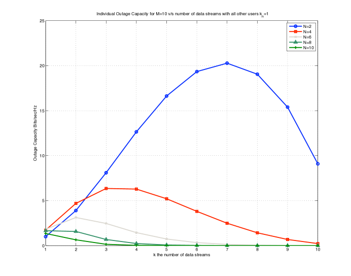
Figure 1: Outage capacity of a single user (1st user) with 10 transmit antennas (M=10) v/s number of data streams with varying N when each of the interferers uses a single data stream $k_{n}=1,\forall\ n\neq 1$.

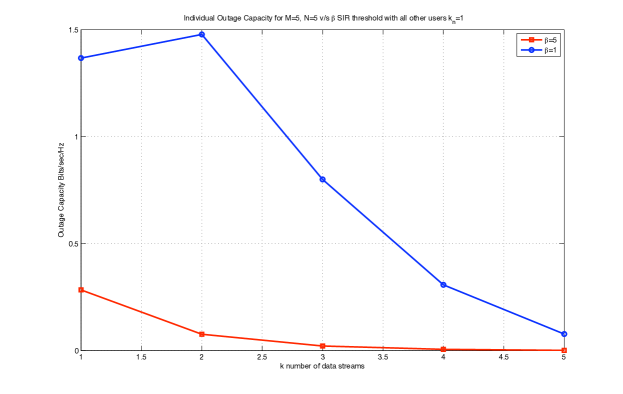
Figure 2: Outage capacity of a single user (1st user) with 5 transmit antennas (M=5) v/s number of data streams for N=5 when each of the interferers uses a single data stream $k_{n}=1,\forall\ n\neq 1$ with varying $\beta$.

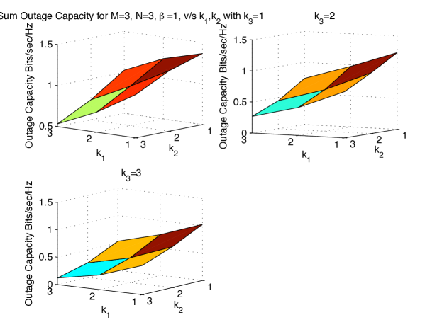
Figure 3: Sum of the outage capacities for $M=3,N=3,\beta=1$ with varying $k_{1},k_{2},k_{3}$.

In this section we provide some numerical examples to illustrate the results obtained in this paper. In Fig. 1 we plot the outage capacity of any one user (say the 1st user) versus the number of data streams $k_{1}$ it uses with $M=10,\beta=1$, when all other users (interferers for 1st user) use a single data stream $k_{n}=1,\ n\neq 1$ for several values of $N$. We see that as $N$ goes towards $M$, $k_{1}=1$ becomes optimal for maximizing the individual outage capacity. Thus, for $\beta\approx 1$, we can see that if $N\approx M$, then $k_{n}=1$ maximizes the individual outage capacity in this case. Next, in Fig. 2 we plot the outage capacity of any one user (say the 1st user) versus the number of data streams $k_{1}$ with $M=5,N=5$, when all other users (interferers for 1st user) use a single data stream $k_{n}=1,\ n\neq 1$ for several values of $\beta$. We can see from Fig. 2 that as $\beta$ increases, the value of $N$ required for having $k_{1}=1$ optimal in terms of maximizing the individual outage capacity decreases. In Fig. 3, we use $N=3,M=3$, i.e. $3$ users with $3$ antennas each, and plot the sum outage capacity as function of number of data streams sent by each user $k_{1},k_{2},k_{3}$. From Fig. 3 it follows that $k_{1}=k_{2}=k_{3}=1$ maximizes the sum outage capacity for $\beta=1$. Here again for $N\approx M$, it is optimal to use $k_{n}=1$.

Appendix A Proof of Theorem 1.

Recall that $C_{n}=Rk_{n}P({\mathsf{SIR}}_{j}^{n}\geq\beta)$, where $P\left(\frac{\frac{s_{j}^{n}}{k_{n}}}{\sum_{m=1,m\neq n}^{N}\frac{1}{k_{m}}\sum_{\ell=1}^{k_{m}}I_{\ell,m}}\geq\beta\right)$, and $s_{j}^{n}\sim\chi^{2}_{2(M-(k_{n}-1))}$, and $I_{\ell,m}\sim\chi^{2}_{2},\ \forall\ \ell,m$. Hence

$$C_{n} = Rk_{n}P\left(\frac{\frac{s_{j}^{n}}{k_{n}}}{\sum_{m=1,m\neq n}^{N}\frac{1}{k_{m}}\sum_{\ell=1}^{k_{m}}I_{\ell,m}}\geq\beta\right),$$ (3)

$$= Rk_{n}{\mathbb{E}}_{I}\left\{\sum_{r=1}^{M-k_{n}+1}\frac{(\beta k_{n}I)^{r}}{r!}e^{-\beta k_{n}I}\right\},\ \text{since}\ s_{j}^{n}\sim\chi^{2}_{2(M-(k_{n}-1))},$$

where $I:=\sum_{m=1,m\neq n}^{N}\frac{1}{k_{m}}\sum_{\ell=1}^{k_{m}}I_{\ell,m}$.

Case 1: $k_{m}=k,\forall\ m\neq n$

In this case $kI\sim\chi^{2}_{2((N-1)k)}$, and hence

$$C_{n} = Rk_{n}{\mathbb{E}}_{I}\left\{\sum_{r=1}^{M-k_{n}+1}\frac{(\frac{\beta k_{n}}{k}kI)^{r}}{r!}e^{-\frac{\beta k_{n}}{k}kI}\right\},$$

$$= Rk_{n}\int_{0}^{\infty}\sum_{r=1}^{M-k_{n}+1}\frac{(\frac{\beta k_{n}}{k}x)^{r}}{r!}e^{-\frac{\beta k_{n}}{k}x}\frac{x^{(N-1)k-1}}{((N-1)k-1)!}e^{-x}dx$$

$$= Rk_{n}\sum_{r=1}^{M-k_{n}+1}\frac{(\frac{\beta k_{n}}{k})^{r}}{r!}\int_{0}^{\infty}\frac{x^{r+(N-1)k-1}}{((N-1)k-1)!}e^{-x(1+\frac{\beta k_{n}}{k})}dx,$$

$$= Rk_{n}\sum_{r=1}^{M-k_{n}+1}\frac{(\frac{\beta k_{n}}{k})^{r}}{(1+\frac{\beta k_{n}}{k})^{r+(N-1)k-1}}\frac{(r+(N-1)k-1)!}{r!((N-1)k-1)!}.$$

Let $B_{n}(k_{n}):=\sum_{r=1}^{M-k_{n}+1}\frac{(\frac{\beta k_{n}}{k})^{r}}{(1+\frac{\beta k_{n}}{k})^{r+(N-1)k-1}}\frac{(r+(N-1)k-1)!}{r!((N-1)k-1)!}$. Hence $C_{n}=Rk_{n}B_{n}(k_{n})$. To show that $C_{n}$ is maximized at $k_{n}=1$, we show that $\frac{B_{n}(k_{n}=p)}{B_{n}(k_{n}=p+1)}\geq\frac{p+1}{p}$ for $p=1,2,\ldots,M$ for large enough $N$. Towards that end, note that

$$\left(\frac{(\frac{\beta p}{k})}{(1+\frac{\beta p}{k})}\right)\geq\left(\frac{(\frac{\beta}{k})}{(1+\frac{\beta}{k})}\right)\ \text{for}\ p=1,2,\ldots,M.$$ (4)

Similarly,

$$\left(\frac{(\frac{\beta p}{k})}{(1+\frac{\beta p}{k})}\right)^{r}\leq 1,\ \text{for}\ p=1,2,\ldots,M.$$ (5)

Now consider

$$\frac{B_{n}(k_{n}=p)}{B_{n}(k_{n}=p+1)} = \frac{\sum_{r=1}^{M-p+1}\frac{(\frac{\beta p}{k})^{r}}{(1+\frac{\beta p}{k})^{r+(N-1)k-1}}\frac{(r+(N-1)k-1)!}{r!((N-1)k-1)!}}{\sum_{r=1}^{M-(p+1)+1}\frac{(\frac{\beta(p+1)}{k})^{r}}{(1+\frac{\beta(p+1)}{k})^{r+(N-1)k-1}}\frac{(r+(N-1)k-1)!}{r!((N-1)k-1)!}},$$

$$= \frac{\frac{1}{(1+\frac{\beta(p)}{k})^{(N-1)k-1}}\sum_{r=1}^{M-p+1}\frac{(\frac{\beta p}{k})^{r}}{(1+\frac{\beta p}{k})^{r}}\frac{(r+(N-1)k-1)!}{r!((N-1)k-1)!}}{\frac{1}{(1+\frac{\beta(p+1)}{k})^{(N-1)k-1}}\sum_{r=1}^{M-p}\frac{(\frac{\beta(p+1)}{k})^{r}}{(1+\frac{\beta(p+1)}{k})^{r}}\frac{(r+(N-1)k-1)!}{r!((N-1)k-1)!}},$$

$$\geq \frac{\frac{1}{(1+\frac{\beta p}{k})^{(N-1)k-1}}\sum_{r=1}^{M-p+1}\frac{(\frac{\beta}{k})^{r}}{(1+\frac{\beta}{k})^{r}}\frac{(r+(N-1)k-1)!}{r!((N-1)k-1)!}}{\frac{1}{(1+\frac{\beta(p+1)}{k})^{(N-1)k-1}}\sum_{r=1}^{M-p}\frac{(r+(N-1)k-1)!}{r!((N-1)k-1)!}},\ \text{from}\ \ (\ref{eq:appaux1}),(\ref{eq:appaux2})$$

$$\geq \frac{\frac{1}{(1+\frac{\beta p}{k})^{(N-1)k-1}}\sum_{r=1}^{M-p+1}\frac{(\frac{\beta}{k})^{M-p+1}}{(1+\frac{\beta}{k})^{M-p+1}}\frac{(r+(N-1)k-1)!}{r!((N-1)k-1)!}}{\frac{1}{(1+\frac{\beta(p+1)}{k})^{(N-1)k-1}}\sum_{r=1}^{M-p}\frac{(r+(N-1)k-1)!}{r!((N-1)k-1)!}},\ \text{since}\ \ \left(\frac{(\frac{\beta}{k})}{(1+\frac{\beta}{k})}\right)\leq 1,$$

$$= \frac{\frac{1}{(1+\frac{\beta p}{k})^{(N-1)k-1}}\frac{(\frac{\beta}{k})^{M-p+1}}{(1+\frac{\beta}{k})^{M-p+1}}\sum_{r=1}^{M-p+1}\frac{(r+(N-1)k-1)!}{r!((N-1)k-1)!}}{\frac{1}{(1+\frac{\beta(p+1)}{k})^{(N-1)k-1}}\sum_{r=1}^{M-p}\frac{(r+(N-1)k-1)!}{r!((N-1)k-1)!}},$$

$$\geq \frac{\frac{1}{(1+\frac{\beta p}{k})^{(N-1)k-1}}\frac{(\frac{\beta}{k})^{M-p+1}}{(1+\frac{\beta}{k})^{M-p+1}}}{\frac{1}{(1+\frac{\beta(p+1)}{k})^{(N-1)k-1}}},$$

$$= \left(\frac{k+\beta(p+1)}{k+\beta p}\right)^{(N-1)k-1}\frac{(\frac{\beta}{k})^{M-p+1}}{(1+\frac{\beta}{k})^{M-p+1}}.$$

Now since $\left(\frac{k+\beta(p+1)}{k+\beta p}\right)>1$, and $\frac{(\frac{\beta}{k})^{M-p+1}}{(1+\frac{\beta}{k})^{M-p+1}}$ is independent of $N$, there exists an $N$ for which $\left(\frac{k+\beta(p+1)}{k+\beta p}\right)^{(N-1)k-1}\frac{(\frac{\beta}{k})^{M-p+1}}{(1+\frac{\beta}{k})^{M-p+1}}\geq\frac{p+1}{p}$ for all $p=1,2,\ldots,M$. Let $N^{\star}$ be the minimum satisfying $\left(\frac{k+\beta(p+1)}{k+\beta p}\right)^{(N-1)k-1}\frac{(\frac{\beta}{k})^{M-p+1}}{(1+\frac{\beta}{k})^{M-p+1}}\geq\frac{p+1}{p}$. Note that for $\beta\geq 1$, $N^{\star}\leq\theta M$, where $\theta>1$ is a constant. Hence we have shown that $C_{n}$ is a decreasing function of $k_{n}$ for $N\geq N^{\star}$, and therefore $k_{n}=1$ maximizes $C_{n},\ \forall\ n=1,2,\ldots,N$.

Case 2: Arbitrary $k_{m}$

In this case because of different scaling factor of $\frac{1}{k_{m}}$, the sum of the interference power $I=\sum_{m=1,m\neq n}^{N}\frac{1}{k_{m}}\sum_{\ell=1}^{k_{m}}I_{\ell,m}$ is not distributed as $\chi^{2}$. The exact distribution of the sum of differently scaled $\chi^{2}$ distributed random variables is known [11], however, is not amenable for analysis and does not yield simple closed form results. To facilitate analysis, we use an approximation on the sum of differently scaled $\chi^{2}$ distributed random variables [12], which is known to be quite accurate.

Lemma 1

Let $X=\sum_{i=1}^{L}a_{i}z_{i}$, where $a_{i}$’s are constants and $z_{i}\sim\chi^{2}(2)$. Then the PDF of $X$ is well approximated by the PDF of the Gamma distributed random variable with parameters $\lambda$ and $1/\alpha$, i.e. $f_{X}(x)=\frac{\alpha^{\lambda}}{\Gamma(\lambda)}e^{-\alpha x}x^{\lambda-1}$, where $\lambda=\frac{1}{2}\frac{(\sum_{i=1}^{L}a_{i})^{2}}{\sum_{i=1}^{L}a^{2}_{i}}$ and $\alpha=\frac{1}{2}\frac{\sum_{i=1}^{L}a_{i}}{\sum_{i=1}^{L}a^{2}_{i}}$.

Using Lemma 1, we can approximate the pdf of $I$ by $f_{I}(x)=\frac{\alpha^{\lambda}}{\Gamma(\lambda)}e^{-\alpha x}x^{\lambda-1}$, where $\alpha=\frac{1}{2}\frac{N\prod_{m=1,m\neq n}^{N}k_{m}}{\sum_{m=1,m\neq n}^{N}k_{m}}$ and $\lambda=\frac{1}{2}\frac{N^{2}\prod_{m=1,m\neq n}^{N}k_{m}}{\sum_{m=1,m\neq n}^{N}k_{m}}$. With this approximation, evaluating the expectation in (3) with respect to $I$, we get

$$C_{n} = Rk_{n}\int_{0}^{\infty}\sum_{r=1}^{M-k_{n}+1}\frac{(\beta k_{n}x)^{r}}{r!}e^{-\beta k_{n}x}\frac{\alpha^{\lambda}x^{\lambda-1}}{\Gamma(\lambda)}e^{-\alpha x}dx,$$

$$= Rk_{n}\alpha^{\lambda}\sum_{r=1}^{M-k_{n}+1}\frac{(\beta k_{n})^{r}}{(\alpha+\beta k_{n})^{r+\lambda-1}}\frac{(r+\lambda-1)!}{r!(\lambda-1)!}.$$

Using a similar argument as for the case of $k_{m}=k,\forall\ m\neq n$, we can show that $C_{n}$ is a decreasing function of $k_{n}$ for sufficiently large $N$. For the sake of brevity we do not repeat the argument here again.

References

• [1] V.Β Tarokh, H.Β Jafarkhani, and A.Β Calderbank, β€œSpace-time block coding for wireless communications: Performance results,” IEEE J. Sel. Areas Commun., vol.Β 17, no.Β 3, pp. 451–460, March 1999.
• [2] E.Β Telatar, β€œCapacity of multi-antenna gaussian channels,” European Trans. on Telecommunications, vol.Β 10, no.Β 6, pp. 585–595, Nov./Dec. 1999.
• [3] P.Β W. Wolniansky, G.Β J. Foschini, G.Β D. Golden, and R.Β A. Valenzuela, β€œV-BLAST: An architecture for realizing very high data rates over the rich-scattering wireless channel,” in ISSSE-1998, Pisa, Italy, Sept. 1998.
• [4] D.Β Tse and P.Β Viswanath, Fundamentals of wireless communication.Β Β Β New York, NY, USA: Cambridge University Press, 2005.
• [5] L.Β Zheng and D.Β Tse, β€œDiversity and multiplexing: A fundamental tradeoff in multiple-antenna channels,” IEEE Trans. Inf. Theory, vol.Β 49, no.Β 5, pp. 1073–1096, May 2003.
• [6] R.Β Vaze and R.Β HeathΒ Jr., β€œTransmission capacity of ad-hoc networks with multiple antennas using transmit stream adaptation and interference cancelation,” IEEE Trans. Inf. Theory, submitted Dec. 2009, available on http://arxiv.org/abs/0912.2630.
• [7] R.Β Blum, β€œMIMO capacity with interference,” IEEE J. Sel. Areas Commun., vol.Β 21, no.Β 5, pp. 793–801, June 2003.
• [8] R.Β Louie, M.Β McKay, and I.Β Collings, β€œSpatial multiplexing with MRC and ZF receivers in ad hoc networks,” in IEEE International Conference on Communications, 2009. ICC ’09., June 2009, pp. 1–5.
• [9] S.Β Weber, X.Β Yang, J.Β Andrews, and G.Β deΒ Veciana, β€œTransmission capacity of wireless ad hoc networks with outage constraints,” IEEE Trans. Inf. Theory, vol.Β 51, no.Β 12, pp. 4091–4102, Dec. 2005.
• [10] N.Β Jindal, J.Β Andrews, and S.Β Weber, β€œRethinking MIMO for wireless networks: Linear throughput increases with multiple receive antennas,” in IEEE International Conference on Communications, 2009. ICC ’09., June 2009, pp. 1–6.
• [11] N.Β Johnson and S.Β Kotz, Continuous univariate distributions.Β Β Β New York, NY, USA: Houghton Mifflin, 1970.
• [12] A.Β H. Feiveson and F.Β C. Delaney, β€œThe distribution and properties of a weighted sum of chi squares,” NASA Technical Note, available on http://ntrs.nasa.gov/archive/nasa/casi.ntrs.nasa.gov/19680015093_1968015093.pdf 1968.
Refer to caption