Gluon spectrum in the glasma from JIMWLK evolution

Abstract

The JIMWLK equation with a “daughter dipole” running coupling is solved numerically, starting from an initial condition given by the McLerran-Venugopalan model. The resulting Wilson line configurations are then used to compute the spectrum of gluons comprising the glasma inital state of a high energy heavy ion collision. The development of a geometrical scaling region makes the spectrum of produced gluons harder. Thus the ratio of the mean gluon transverse momentum to the saturation scale grows with energy. Also the total gluon multiplicity increases with energy slightly faster than the saturation scale squared.

I Introduction

Particle production in the initial stage of a high energy heavy collision, at RHIC or the LHC, is dominated by the small $x$ gluonic degrees of freedom in the nuclear wavefunctions. When the dynamics of these gluons is dominated by a semihard saturation scale $Q_{\mathrm{s}}$ it is possible to understand the initial particle production in terms of weak coupling, first principles QCD. This can be done in the framework of the CGC effective theory (for reviews see e.g. Iancu:2003xm ; *Weigert:2005us; *Gelis:2010nm; *Lappi:2010ek), where the calculation is organized in terms of the classical gluon field for the small $x$ degrees of freedom, radiated from an effective color source representing the larger $x$ partons. This generic division only relies on the large energy, which, due to time dilation, makes the large $x$ degrees of freedom evolve slowly, and on gluon saturation and weak coupling, which guarantees the validity of the classical field approximation.

The energy (or $x$) dependence of the gluonic degrees of freedom is encoded in the JIMWLK Jalilian-Marian:1997xn ; *Jalilian-Marian:1997jx; *Jalilian-Marian:1997gr; *Jalilian-Marian:1997dw; *JalilianMarian:1998cb; *Iancu:2000hn; *Iancu:2001md; *Ferreiro:2001qy; *Iancu:2001ad; *Mueller:2001uk renormalization group equation, which is obtained by successively integrating out the quantum fluctuations around the classical field into the color source. The small $x$ gluonic degrees of freedom are most conveniently described in terms of Wilson lines in the classical field. The correlators of these Wilson lines can be probed experimentally by scattering a dilute probe off the CGC, such as in DIS or pA collisions at forward rapidity. Many phenomenological applications of this framework use the BK Balitsky:1995ub ; *Kovchegov:1999yj equation, which can be derived from JIMWLK in a mean field approximation.

A collision of two objects described in the CGC framework can also be understood in terms of classical gluon fields, the glasma fields Lappi:2006fp . They start off for $\tau\lesssim 1/Q_{\mathrm{s}}$ as longitudinal chromoelectric and magnetic fields and evolve for $\tau\gtrsim 1/Q_{\mathrm{s}}$ into modes that can be described as gluons with transverse momenta of order $Q_{\mathrm{s}}$. The basic structure of the glasma fields has been known for some time Kovner:1995ts . They can be obtained from a solution of the Classical Yang-Mills (CYM) equations of motion starting from an initial condition expressed in terms of the Wilson lines mentioned above. The full equations have not been solved analytically, but there has been a significant amount of work to develop numerical solutions. So far, however, the numerical CYM Krasnitz:1998ns ; *Krasnitz:2001qu; *Krasnitz:2003jw; Lappi:2003bi calculations have been performed using the Wilson lines from the MV model McLerran:1994ni ; *McLerran:1994ka; *McLerran:1994vd, in stead of the full solution of the JIMWLK equation. The only calculations of gluon production to include the dynamics of high energy evolution have been done using a solution of the BK equation in a $k_{T}$-factorized approximation Gelis:2006tb ; Albacete:2007sm ; Dusling:2009ni ; Albacete:2010bs ; *Albacete:2010ad. Since $k_{T}$-factorization does not correctly give the initial gluon spectrum, or multiplicity, for the collision of two dense systems (the “AA” case) Blaizot:2008yb ; Blaizot:2010kh ; Levin:2010zs , these calculations are insufficient to give a full picture of the initial gluonic matter produced in a heavy ion collision.

The goal of this paper is to take the missing step of combining JIMWLK evolution with a full CYM calculation of gluon production in a heavy ion collision. The JIMWLK equation is solved numerically, using a (“daughter dipole”) running coupling constant. The resulting Wilson line configurations are then used as initial conditions in a numerical computation of the spectrum of gluons produced in a collision of two sheets of CGC. The point of view taken in this paper is that the MV model should be a reasonable initial condition for the evolution around RHIC energies. We shall show explicitly how, starting from this initial condition, the effect of JIMWLK evolution is the creation of a geometrical scaling region for momenta $k_{T}\gtrsim Q_{\mathrm{s}}$, with a gluon spectrum that is harder than in the initial condition. This feature is carried over from the wavefunction to the spectrum of gluons in the glasma, making the glasma initial state more energetic at higher energies than a straightforward extrapolation of the MV model.

The numerical method for solving the JIMWLK equation is the one developed in Rummukainen:2003ns and the one for solving the CYM equations of motion that used e.g. in Refs Krasnitz:1998ns ; *Krasnitz:2001qu; *Krasnitz:2003jw; Lappi:2003bi . We will thus only briefly describe them in Sec. II, and refer the reader e.g. to Refs. Rummukainen:2003ns ; Lappi:2009xa ; Blaizot:2010kh for a more extensive discussion. We will then characterize our results for the JIMWLK equation in Sec. III and for the CYM calculation in Sec. IV, before discussing phenomenological context and future directions in Sec. V.

The BK/JIMWLK evolution is most conventionally analyzed in terms of the fundamental representation saturation scale, which we denote by $Q_{\mathrm{s}}$. Gluon production, on the other hand, is expected to be dominated by the adjoint representation saturation scale which we denote $\widetilde{Q}_{\mathrm{s}}$. These are related by a simple color factor $\widetilde{Q}_{\mathrm{s}}^{2}=[C_{\mathrm{A}}/C_{\mathrm{F}}]Q_{\mathrm{s}}^{2}=[2{N_{\mathrm{c}}}^{2}/({N_{\mathrm{c}}}^{2}-1)]Q_{\mathrm{s}}^{2}$. The exact definition of $Q_{\mathrm{s}}$ used here is given in terms of the coordinate space Wilson line correlator in Eq. (11).

II Solving JIMWLK and the CYM equations of motion

The JIMWLK equation describes the rapidity (or energy) evolution of the probability distribution for Wilson lines. In the CGC framework large $x$ degrees of freedom are described by static color charges, which serve as sources for a classical color field. Most physical observables can be expressed in terms of Wilson lines formed from the color field (in the covariant gauge, for a source moving in the positive $z$ direction)

$$U({\mathbf{x}_{T}})=P\exp\left\{i\int\,\mathrm{d}x^{-}A^{+}_{\mathrm{cov}}({\mathbf{x}_{T}},x^{-})\right\}.$$ (1)

These Wilson lines are random SU(3) matrices from a probability distribution $W_{y}[U({\mathbf{x}_{T}})]$, which depends on the rapidity cutoff $y$ that separates the large $x$ color sources from the small $x$ classical field. As the energy is increased, successive layers of quantum fluctuations have to be integrated into the probability distribution. This leads to the JIMWLK renormalization group equation

$$\partial_{y}W_{y}[U]=-\frac{1}{2}\frac{\alpha_{\mathrm{s}}}{\pi^{2}}\int\limits_{{\mathbf{x}_{T}}{\mathbf{y}_{T}}{\mathbf{z}_{T}}}\frac{\delta}{\delta A_{\mathrm{cov}}^{c+}({\mathbf{x}_{T}})}\\ \bigg{[}\left(1-U^{\dagger}({\mathbf{x}_{T}})U({\mathbf{z}_{T}})\right)^{ca}\left(1-U^{\dagger}({\mathbf{y}_{T}})U({\mathbf{z}_{T}})\right)^{ba}\\ \frac{({\mathbf{x}_{T}}-{\mathbf{z}_{T}})\cdot({\mathbf{y}_{T}}-{\mathbf{z}_{T}})}{({\mathbf{x}_{T}}-{\mathbf{z}_{T}})^{2}({\mathbf{y}_{T}}-{\mathbf{z}_{T}})^{2}}\frac{\delta}{\delta A_{\mathrm{cov}}^{b+}({\mathbf{y}_{T}})}W_{y}[U]\bigg{]},$$ (2)

which describes the energy dependence of this probability distribution. This evolution equation can be written in a Langevin form for the rapidity evolution of the Wilson lines

$$U_{y+\,\mathrm{d}y}({\mathbf{x}_{T}})=U_{y}({\mathbf{x}_{T}})e^{i\alpha^{a}({\mathbf{x}_{T}},y)t^{a}},$$ (3)

where at each timestep the Wilson line is rotated in color space by

$$\alpha^{a}({\mathbf{x}_{T}},y)=-\int\limits_{{\mathbf{z}_{T}}}\bigg{[}\frac{i\alpha_{\mathrm{s}}\,\mathrm{d}y}{2\pi^{2}({\mathbf{x}_{T}}-{\mathbf{z}_{T}})^{2}}\,\mathrm{Tr}\,\left[T^{a}\tilde{U}^{\dagger}({\mathbf{x}_{T}})\tilde{U}({\mathbf{z}_{T}})\right]$$

$$\,\,+\frac{\sqrt{\alpha_{\mathrm{s}}\,\mathrm{d}y}}{\pi}\frac{(x-z)^{i}}{({\mathbf{x}_{T}}-{\mathbf{z}_{T}})^{2}}\left[1-U^{\dagger}({\mathbf{x}_{T}})U({\mathbf{z}_{T}})\right]^{ab}\eta_{i}^{b}({\mathbf{z}_{T}})\bigg{]},$$ (4)

with a random noise

$$\langle\eta_{i}^{a}({\mathbf{x}_{T}},y)\eta_{j}^{b}({\mathbf{y}_{T}},y^{\prime})\rangle=\delta^{ij}\delta^{ab}\delta^{2}({\mathbf{x}_{T}}-{\mathbf{y}_{T}})\delta(y-y^{\prime}).$$ (5)

Here $\tilde{U}$ denotes the matrix in the adjoint representation, and $T^{a}$ are the adjoint representation generators. This numerical procedure relies on the factorization of the JIMWLK kernel into a product of two terms, depending only on the coordinate pairs ${\mathbf{x}_{T}},{\mathbf{z}_{T}}$ and ${\mathbf{y}_{T}},{\mathbf{z}_{T}}$ (the “daughter dipoles”).

Published numerical solutions of the JIMWLK equation so far Rummukainen:2003ns ; Kovchegov:2008mk have used a fixed coupling constant $\alpha_{\mathrm{s}}$. This gives an evolution speed (increase of $Q_{\mathrm{s}}$ with energy) that is too fast to be phenomenologically reasonable, so it is essential to use a running coupling constant here. There has been much discussion on the best running coupling prescription for BK/JIMWLK evolution in the literature Kovchegov:2006vj ; Balitsky:2006wa ; Albacete:2007yr . The running coupling constant resums a subset of the NLO corrections to BK/JIMWLK evolution, and different prescriptions correspond to resumming a different subset of them. Thus there is no unique “correct” way to set the scale of the coupling constant, although it has been argued Albacete:2007yr that the Balitsky prescription Balitsky:2006wa minimizes the effect of other NLO corrections. The numerical Langevin method of solving the JIMWLK equation relies on factorizing the JIMWLK kernel into a product of two factors that only depend on the sizes of the “daughter” dipole ${\mathbf{x}_{T}}-{\mathbf{z}_{T}}$ in Eq. (4). Thus implementing the preferred prescription of Balitsky:2006wa would be difficult in a numerical solution of JIMWLK. We therefore use in this work the ad hoc “daughter dipole” prescription, where the magnitude of the coupling in Eq. (4) only depends on ${\mathbf{x}_{T}}-{\mathbf{z}_{T}}$. One also has to regulate the Landau pole in the coupling constant, which we do in a smooth way at a scale $\mu_{0}$ by taking

$$\alpha_{\mathrm{s}}(r)=\frac{12\pi}{\left(33-2{N_{\mathrm{F}}}\right)\ln\left[\left(\mu_{0}^{2}/\Lambda^{2}\right)^{1/c}+\left(r^{2}\Lambda^{2}/4\right)^{-1/c}\right]^{c}}$$ (6)

with ${N_{\mathrm{F}}}=3$ and $c=0.2$. The value of the frozen coupling is $\alpha_{0}=\frac{12\pi}{(33-2{N_{\mathrm{F}}})\ln(\mu_{0}^{2}/\Lambda)}.$ The scale $\Lambda$ in the coupling is parametrically of the order of $\Lambda_{\mathrm{QCD}}$, but the exact value that should be used is scheme dependent. In the running coupling BK fit to DIS data Albacete:2009fh ; *Albacete:2010sy the scale is taken as a fit parameter and the data is found to prefer a smaller value $\Lambda^{2}=\Lambda_{\mathrm{QCD}}^{2}/6.5,$ which we will assume here.

The initial Wilson lines at $y=0$ are taken from the MV model, using the method discussed in more detail e.g. in Ref. Lappi:2007ku . After a given number of iterations of the Langevin equation (4) (we use a step size $\,\mathrm{d}y=0.0001\pi^{2}/\alpha_{0}$) one then obtains the configurations at a higher rapidity $y$. This is done separately for two independent configurations, corresponding to the two colliding nuclei. In this work we only consider the symmetric situation of particle production at midrapidity, thus we evolve both nuclei starting from the same $Q_{\mathrm{s0}}$ and for the same interval in $y$.

Denoting the two nuclei as $A$ and $B$ one proceeds by constructing the light cone gauge fields corresponding to the Wilson lines as

$$A_{i}^{A,B}=\frac{i}{g}U^{\dagger}_{A,B}\partial_{i}U_{A,B}.$$ (7)

The CYM equations of motion for the glasma fields are then solved as an initial value problem with initial conditions Kovner:1995ts

$$\left.A^{i}\right|_{\tau=0^{+}} = A_{A}^{i}+A_{B}^{i},$$ (8)

$$\left.A^{\eta}\right|_{\tau=0^{+}} = \frac{ig}{2}[A_{A}^{i},A_{B}^{i}].$$ (9)

At a given proper time of ($\tau=12/\widetilde{Q}_{\mathrm{s}}$ in our case) these fields are then Fourier-decomposed into ${\mathbf{k}_{T}}$-modes to determine the spectrum of the produced gluons.

III Results for JIMWLK

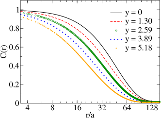
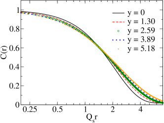
Figure 1: Wilson line correlator (10) in coordinate space; in lattice units (above) and as a function of the scaling variable $rQ_{\mathrm{s}}$ (below).

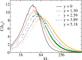
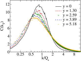
Figure 2: Wilson line correlator (10) (dipole cross section) in momentum space; as s function of $k_{T}L$ (above) and of the scaling variable $k/Q_{\mathrm{s}}$ (below).

The most elementary observable to monitor during the evolution is the Wilson line correlator

$$C(r=|{\mathbf{x}_{T}}-{\mathbf{y}_{T}}|)=\frac{1}{{N_{\mathrm{c}}}}\left\langle\,\mathrm{Tr}\,U^{\dagger}({\mathbf{x}_{T}})U({\mathbf{y}_{T}})\right\rangle.$$ (10)

The related dipole cross section $2\int\,\mathrm{d}^{2}{\mathbf{b}_{T}}(1-C(r))$ appears directly in the expression for the inclusive DIS cross section and is therefore of interest in itself. The correlator varies between the values 1 at $r=0$ and 0 at large $r$, providing a natural way to define the saturation scale as the inverse of the correlation length of the Wilson lines as an intermediate scale between these two regimes. We adopt the definition, as in Kowalski:2003hm , of the fundamental representation $Q_{\mathrm{s}}$ by the criterion

$$C(r=\sqrt{2}/Q_{\mathrm{s}})=e^{-1/2}.$$ (11)

Note that while for a Gaussian (“GBW”Golec-Biernat:1998js ) correlator this definition is equivalent to the momentum space one used in Ref. Lappi:2007ku , they need not give exactly the same values in the general case.

In $k_{T}$-factorized calculations of gluon production in pA collisions one needs the unintegrated gluon distribution of the dense target. This is obtained from the the Fourier transform of Eq. (10) multiplied by $k_{T}^{2}$

$$C({\mathbf{k}_{T}})={\mathbf{k}_{T}}^{2}\int\,\mathrm{d}^{2}{\mathbf{r}_{T}}e^{i{\mathbf{k}_{T}}\cdot{\mathbf{r}_{T}}}C({\mathbf{r}_{T}}).$$ (12)

The typical behavior of the unintegrated distribution (12) is to start at zero for small $k_{T}$ and have maximum around $k_{T}\sim Q_{\mathrm{s}}$.

In the MV model the unintegrated gluon distribution behaves as $C(k_{T})\sim 1/k_{T}^{2}$ for large $k_{T}$, which corresponds to the integrated gluon distribution $xg(x,Q^{2})$ behaving as $\sim\ln Q^{2}$. The main effects of JIMWLK/BK evolution are the increase of the characteristic scale $Q_{\mathrm{s}}$ with energy and and making the functional form of the unintegrated distribution less steep, $\sim 1/k_{T}^{2\gamma}$. For fixed coupling the anomalous dimension is Iancu:2002tr ; *Mueller:2002zm $\gamma\approx 0.63$ and for running coupling numerical solutions Albacete:2004gw of the BK equation give $\gamma\approx 0.85$. Our present calculation is done on a linear (as opposed to logarithmic) lattice, and cannot go to very large momenta before lattice ultraviolet cutoff effects are felt in the spectrum. Therefore one cannot hope to get a very good numerical evaluation of the anomalous dimension. The change in the behavior of the unintegrated gluon distribution is, however, clearly observable. The Wilson line correlators at different rapidities are shown in Fig. 1 in coordinate space and in Fig. 2 in momentum space, both in lattice units and a functions of the scaling variables $rQ_{\mathrm{s}}$ and $k/Q_{\mathrm{s}}$. Both the increase of $Q_{\mathrm{s}}$ and the development of a geometric scaling region are very well visible.

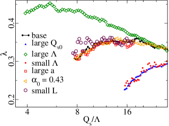
Figure 3: The evolution speed $\lambda=\,\mathrm{d}\ln Q_{\mathrm{s}}^{2}(x)/\,\mathrm{d}\ln 1/x$ as a function of the saturation scale $Q_{\mathrm{s}}$. The parameter values corresponding to the labels are detailed in Table 1.

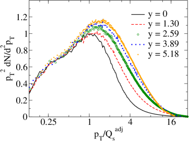
Figure 4: Gluon spectrum at different energies, labeled by the rapidity interval of evolution starting from the MV initial condition at $y=0$. The momentum is scaled by the saturation scale $Q_{\mathrm{s}}$ corresponding to the rapidity in question.

Configuration	$N_{\perp}$	$\widetilde{Q}_{\mathrm{s0}}L$	$\mu_{0}L$	$\Lambda L$
Base	1024	68	15	6
Large $Q_{\mathrm{s0}}$	1024	136	15	6
Large $\Lambda$	1024	68	30	12
Small $\Lambda$	1024	68	7.5	3
Large $a$	512	68	15	6
Small $\alpha_{0}$	1024	68	30	6
Small $L$	512	34	7.5	3
Small $L,a$	1024	34	7.5	3

Table 1: The values of the numerical parameters used in our simulation sets. For $\mu_{0}/\Lambda=2.5$ the coupling is frozen at the value $\alpha_{0}=0.762$ and for $\mu_{0}/\Lambda=5$ at $\alpha_{0}=0.434$.

The values used in the different sets of numerical computations in this paper are summarized in Table 1. The dependence of physical observables on the collision energy and rapidity depends most of all on the speed of evolution, conventionally parametrized as

$$\lambda=\frac{\,\mathrm{d}\ln Q_{\mathrm{s}}^{2}(y)}{\,\mathrm{d}y}.$$ (13)

At fixed coupling $\lambda\sim\alpha_{\mathrm{s}}$, and at running coupling the speed is expected to be proportional to $\alpha_{\mathrm{s}}(Q_{\mathrm{s}}^{2})$. Thus the evolution speed is controlled by the relation of the initial saturation scale to the QCD scale controlling the running of the coupling, $\widetilde{Q}_{\mathrm{s0}}/\Lambda$. In a physically realistic case we would like to start the evolution at a scale corresponding to midrapidity at RHIC energies, i.e. $\widetilde{Q}_{\mathrm{s0}}\approx 1.1\ \textrm{GeV}$ Lappi:2007ku , corresponding to $\widetilde{Q}_{\mathrm{s0}}/\Lambda\approx 11$, i.e. $Q_{\mathrm{s0}}/\Lambda\approx 7.6$. Assuming the transverse area to be $L^{2}=140\ \textrm{fm}^{2}$ this leads to $\widetilde{Q}_{\mathrm{s0}}L\approx 68$. These correspond to the “base” set of values in Table 1 and used in Figs. 1, 2 and 4. To test the effect of the initial scale on the speed of evolution we also show results with two different values of $\widetilde{Q}_{\mathrm{s0}}/\Lambda$. The change in $\widetilde{Q}_{\mathrm{s0}}/\Lambda$ is obtained by increasing $\widetilde{Q}_{\mathrm{s0}}$ by a factor of 2 and keeping all other parameters fixed. Alternatively $\Lambda$ is decreased or increased by a factor of 2, with everything else fixed. The value at which the coupling freezes without altering the dynamics at higher momentum scales can be altered by changing $\mu_{0}$. The sensitivity of the calculation to lattice effects has been tested by changing the lattice spacing $a$ (i.e. the lattice UV cutoff $\sim 1/a$) and the physical volume $L=N_{\perp}a$ by a factor of two, with all the other dimensionful parameters fixed.

The initial conditions in the MV model are constructed Lappi:2007ku as a product of $N_{y}=100$ infinitesimal Wilson lines, with the MV model color charge density parameter $g^{2}\mu$ adjusted to provide the desired saturation scale. The evolution speed for the different configurations is shown in Fig. 3, as a function of $Q_{\mathrm{s}}/\Lambda$. This confirms the expectation that starting with a lower $Q_{\mathrm{s0}}/\Lambda$ results in a faster initial evolution. The phenomenologically preferred evolution speed $\lambda\lesssim 0.3$ is only reached with an initial saturation scale that is higher than the above estimates corresponding to RHIC energy. Note, however, that this is affected by the uncertainty concerning the correct value of $\Lambda$ in this running coupling scheme.

IV Results for the gluon spectrum

We then take the Wilson line configurations from the JIMWLK evolution and, as discussed in Sec. II, use them as initial conditions for the solution of the CYM equations of motion. The gluon spectrum resulting from the calculation is shown in Fig. 4. One can see that the gluon spectrum gets gradually harder as one moves from the initial condition into the geometric scaling regime. In the rapidity interval considered here the total multiplicity and transverse energy of the gluons are still finite. This is to be contrasted with the case of fixed coupling where, for an unintegrated gluon distribution behaving as $C(k_{T})\sim k_{T}^{-2\gamma}$ the produced gluon spectrum would behave as $\,\mathrm{d}N/\,\mathrm{d}^{2}{\mathbf{p}_{T}}\sim p_{T}^{-4\gamma}.$ If the geometric scaling behavior continued to arbitrary large $k_{T}$ this would result in an ultraviolet divergent transverse energy for $\gamma<0.75,$ including the fixed coupling value $\sim 0.63$. In practice the geometrical scaling region does not extend up to infinite $k_{T}$, but a very hard gluon spectrum could be difficult to reconcile with the observed transverse energy of the later stages of the quark gluon plasma.

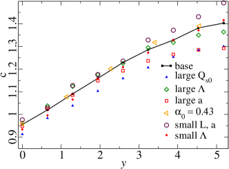
Figure 5: Gluon liberation coefficient as a function of collision energy, parametrized by the rapidity interval of evolution from the initial scale.

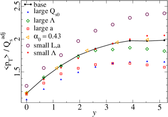
Figure 6: Mean gluonic transverse momentum as a function of collision energy..

The dominant transverse momentum scale of the produced gluon spectrum is expected to be the adjoint representation $\widetilde{Q}_{\mathrm{s}}$. It is convenient to parametrize the gluon spectrum by the dimensionless “liberation coefficient”Mueller:1999fp ; *Mueller:2002kw; Kovchegov:2000hz $c$ proportional to the total gluon multiplicity

$$\frac{\,\mathrm{d}N_{\mathrm{init.}g}}{\,\mathrm{d}^{2}{\mathbf{x}_{T}}\,\mathrm{d}y}=c\frac{C_{\mathrm{F}}\widetilde{Q}_{\mathrm{s}}^{2}}{2\pi^{2}\alpha_{\mathrm{s}}},$$ (14)

and the mean transverse momentum of the produced gluons $\langle p_{T}\rangle$. For a more thorough discussion on relating these values to the measured charged particle multiplicities we refer the reader to e.g. Lappi:2011gu .

The values of $c$ and $\langle p_{T}\rangle/\widetilde{Q}_{\mathrm{s}}$ for different amounts of evolution are plotted in Figs. 5 and 6. We see that, as expected, the harder $k_{T}$-dependence in the initial wavefunctions leads to a harder spectrum of produced gluons, as evidenced by the increase of $\langle p_{T}\rangle/\widetilde{Q}_{\mathrm{s}}$ from the initial condition. This increase does, however, seem to saturate after $y\approx 3$. This indicates that the functional form starts to settle towards a new scaling characteristic of JIMWLK evolution, where the anomalous dimension $\gamma<1$ leads to a harder spectrum than in the MV model. The mean transverse momentum of the gluons in the glasma, scaled by $Q_{\mathrm{s}}$, increases from $\sim 1$ for the MV model initial condition to around $\sim 1.5$.

A somewhat less expected feature is the increase of the scaled multiplicity $c$ seen in Fig. 5. This is seen also in the shape of the scaled spectrum in Fig. 4, where new gluons are added for $p_{T}\gtrsim 2\widetilde{Q}_{\mathrm{s}}$, but the shape for $p_{T}\lesssim\widetilde{Q}_{\mathrm{s}}$ changes very little. This observation could, as in Ref. Blaizot:2010kh , be interpreted as a difference between “initial” and “final” state interactions. At high transverse momentum $p_{T}\gtrsim 2/\widetilde{Q}_{\mathrm{s}}$ the produced gluon spectrum reflects the unintegrated gluon distributions in the colliding projectiles. Thus $k_{T}$-factorization works in this regime, and the spectrum gets harder because of the development of the geometrical scaling window. The shape of the spectrum for $p_{T}\lesssim\widetilde{Q}_{\mathrm{s}}$, on the other hand, is a result of nonlinear interactions in the glasma stage, which render the spectrum IR finite. These interactions are not captured in the $k_{T}$-factorized formalism.

Both $c$ and $\langle p_{T}\rangle$ are smaller for the configurations where $Q_{\mathrm{s}}a$ is large (“small $a$” and “large $Q_{\mathrm{s}}$”), which implies a strong dependence on the lattice ultraviolet cutoff $1/a$. This is to be contrasted with Fig. 3, where the evolution speed $\lambda$ showed no significant dependence on the UV cutoff. Testing this by further decreasing $a$ with the same $L$ would become prohibitively expensive for this study. We can, however, achieve smaller values of $Q_{\mathrm{s}}a$ by decreasing the size of the system, i.e. $Q_{\mathrm{s}}L$. Making $Q_{\mathrm{s0}}L$ smaller is eventually limited by the goal of staying in the strong field regime already for the initial rapidity.

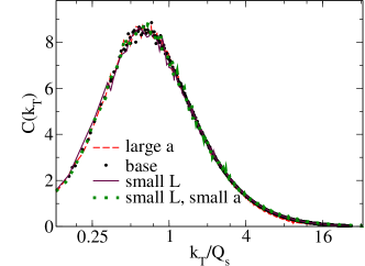
Figure 7: The Wilson line correlator after $5.2$ units in rapidity. The points and the dashed line differ only by the value of the lattice spacing $a$ used. The dotted and solid line likewise differ only by the value of $a$, and are obtained with $L$ half of the first ones. For the parameter values used see Table 1.

The effect of the lattice UV cutoff is demonstrated further in Figs. 7 and 8. They show the unintegrated gluon distribution (Fig. 7) and the produced gluon spectrum (Fig. 8) after $5.2$ rapidity units of evolution for two different values of $Q_{\mathrm{s0}}L$, with two different values of $Q_{\mathrm{s0}}a$ each, keeping the other parameters of the evolution the same. One can see that with the new phase space opening up at smaller $a$ the unintegrated gluon distribution is mostly unaffected. The produced gluon spectrum, on the other hand, increases in the high $p_{T}$ tail. Thus the produced gluon spectrum is more sensitive to the lattice regularization than the JIMWLK evolution itself. One consequence of this is that the leveling off of the increase in $\langle p_{T}\rangle/Q_{\mathrm{s}}$ at high rapidity, seen in Fig. 6, could be influenced by lattice cutoff effects.

V Discussion

We have, for the first time, used the solution of nonlinear the high energy evolution equations in a calculation of gluon production in the initial stage of a heavy ion collision without resorting to a $k_{T}$-factorized approximation. This enables us to compute the gluon multiplicity and transverse energy density without ambiguities related to the normalization and without additional infrared cutoffs. It has been seen that the effect of JIMWLK evolution is to make the gluon spectrum harder, leading to a growth of the total multiplicity that is slightly faster than $\sim Q_{\mathrm{s}}^{2}$ and a gluon mean $p_{T}$ that grows faster than $Q_{\mathrm{s}}$. The resulting gluon spectrum in the glasma, shown in Fig. 4 is the main result of this paper.

The numerical calculation confirms that, as expected from studies of the BK equation, introducing a running coupling slows down the evolution to a speed more consistent with experimental observations. At fixed coupling, numerical JIMWLK evolution is known to be very sensitive to the lattice ultraviolet cutoff. With running coupling the speed of evolution becomes essentially independent of the UV cutoff. However, when the solution is used as an input for a calculation of the gluon spectrum of the initial glasma phase of heavy ion collisions, the lattice spacing dependence again becomes stronger. A full systematic continuum extrapolation is, however, left for future work. Effects of higher order corrections to JIMWLK/BK evolution could significantly modify the physics at $k_{T}\gtrsim Q_{\mathrm{s}}.$ This would have a larger effect on the spectrum of gluons in the glasma than expected just from the speed of the evolution.

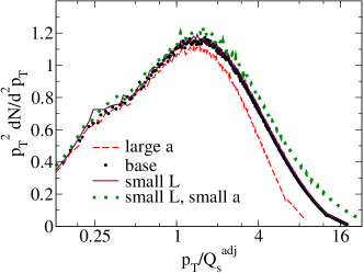
Figure 8: Scaled gluon spectrum after $5.2$ units in rapidity. The labels are as in Fig. 7.

The inclusion of NLO effects in our calculation has, by reasons of of numerical practicality, been limited to a “daughter dipole” prescription for the running coupling. Incorporating more of the NLO corrections to JIMWLK/BK evolution into the could have a much larger effect on the gluon spectrum in a nucleus-nucleus collisions than on, say, the total DIS cross section. Another, separate but phenomenologically extremely topical issue that can be addressed in this same framework, are long range rapidity correlations in the glasma Dumitru:2008wn ; Dusling:2009ni ; Dumitru:2010iy . The calculation of the “ridge” correlation in the glasma proceeds in a similar fashion as the one performed in this paper, but is left for future work.

References

- (1) E. Iancu and R. Venugopalan in Quark gluon plasma (R. Hwa and X. N. Wang, eds.). World Scientific, 2003. arXiv:hep-ph/0303204
- (2) H. Weigert Prog. Part. Nucl. Phys. 55 (2005) 461 [arXiv:hep-ph/0501087]
- (3) F. Gelis, E. Iancu, J. Jalilian-Marian and R. Venugopalan Ann.Rev.Nucl.Part.Sci. 60 (2010) 463 [arXiv:1002.0333 [hep-ph]]
- (4) T. Lappi Int.J.Mod.Phys. E20 (2011) 1 [arXiv:1003.1852 [hep-ph]]
- (5) J. Jalilian-Marian, A. Kovner, L. D. McLerran and H. Weigert Phys. Rev. D55 (1997) 5414 [arXiv:hep-ph/9606337]
- (6) J. Jalilian-Marian, A. Kovner, A. Leonidov and H. Weigert Nucl. Phys. B504 (1997) 415 [arXiv:hep-ph/9701284]
- (7) J. Jalilian-Marian, A. Kovner, A. Leonidov and H. Weigert Phys. Rev. D59 (1999) 014014 [arXiv:hep-ph/9706377]
- (8) J. Jalilian-Marian, A. Kovner and H. Weigert Phys. Rev. D59 (1999) 014015 [arXiv:hep-ph/9709432]
- (9) J. Jalilian-Marian, A. Kovner, A. Leonidov and H. Weigert Phys. Rev. D59 (1999) 034007 [arXiv:hep-ph/9807462]
- (10) E. Iancu, A. Leonidov and L. D. McLerran Nucl. Phys. A692 (2001) 583 [arXiv:hep-ph/0011241]
- (11) E. Iancu and L. D. McLerran Phys. Lett. B510 (2001) 145 [arXiv:hep-ph/0103032]
- (12) E. Ferreiro, E. Iancu, A. Leonidov and L. McLerran Nucl. Phys. A703 (2002) 489 [arXiv:hep-ph/0109115]
- (13) E. Iancu, A. Leonidov and L. D. McLerran Phys. Lett. B510 (2001) 133 [arXiv:hep-ph/0102009]
- (14) A. H. Mueller Phys. Lett. B523 (2001) 243 [arXiv:hep-ph/0110169]
- (15) I. Balitsky Nucl. Phys. B463 (1996) 99 [arXiv:hep-ph/9509348]
- (16) Y. V. Kovchegov Phys. Rev. D60 (1999) 034008 [arXiv:hep-ph/9901281]
- (17) T. Lappi and L. McLerran Nucl. Phys. A772 (2006) 200 [arXiv:hep-ph/0602189]
- (18) A. Kovner, L. D. McLerran and H. Weigert Phys. Rev. D52 (1995) 3809 [arXiv:hep-ph/9505320]
- (19) A. Krasnitz and R. Venugopalan Nucl. Phys. B557 (1999) 237 [arXiv:hep-ph/9809433]
- (20) A. Krasnitz, Y. Nara and R. Venugopalan Phys. Rev. Lett. 87 (2001) 192302 [arXiv:hep-ph/0108092]
- (21) A. Krasnitz, Y. Nara and R. Venugopalan Nucl. Phys. A727 (2003) 427 [arXiv:hep-ph/0305112]
- (22) T. Lappi Phys. Rev. C67 (2003) 054903 [arXiv:hep-ph/0303076]
- (23) L. D. McLerran and R. Venugopalan Phys. Rev. D49 (1994) 2233 [arXiv:hep-ph/9309289]
- (24) L. D. McLerran and R. Venugopalan Phys. Rev. D49 (1994) 3352 [arXiv:hep-ph/9311205]
- (25) L. D. McLerran and R. Venugopalan Phys. Rev. D50 (1994) 2225 [arXiv:hep-ph/9402335]
- (26) F. Gelis, A. M. Stasto and R. Venugopalan Eur. Phys. J. C48 (2006) 489 [arXiv:hep-ph/0605087]
- (27) J. L. Albacete Phys. Rev. Lett. 99 (2007) 262301 [arXiv:0707.2545 [hep-ph]]
- (28) K. Dusling, F. Gelis, T. Lappi and R. Venugopalan Nucl. Phys. A836 (2010) 159 [arXiv:0911.2720 [hep-ph]]
- (29) J. L. Albacete and C. Marquet Phys.Lett. B687 (2010) 174 [arXiv:1001.1378 [hep-ph]]
- (30) J. L. Albacete and A. Dumitru arXiv:1011.5161 [hep-ph]
- (31) J.-P. Blaizot and Y. Mehtar-Tani Nucl. Phys. A818 (2009) 97 [arXiv:0806.1422 [hep-ph]]
- (32) J. P. Blaizot, T. Lappi and Y. Mehtar-Tani Nucl. Phys. A846 (2010) 63 [arXiv:1005.0955 [hep-ph]]
- (33) E. Levin Phys.Rev. D82 (2010) 101704 [arXiv:1010.4630 [hep-ph]]
- (34) K. Rummukainen and H. Weigert Nucl. Phys. A739 (2004) 183 [arXiv:hep-ph/0309306]
- (35) T. Lappi, S. Srednyak and R. Venugopalan JHEP 01 (2010) 066 [arXiv:0911.2068 [hep-ph]]
- (36) Y. V. Kovchegov, J. Kuokkanen, K. Rummukainen and H. Weigert Nucl. Phys. A823 (2009) 47 [arXiv:0812.3238 [hep-ph]]
- (37) Y. V. Kovchegov and H. Weigert Nucl. Phys. A784 (2007) 188 [arXiv:hep-ph/0609090]
- (38) I. Balitsky Phys. Rev. D75 (2007) 014001 [arXiv:hep-ph/0609105]
- (39) J. L. Albacete and Y. V. Kovchegov Phys. Rev. D75 (2007) 125021 [arXiv:0704.0612 [hep-ph]]
- (40) J. L. Albacete, N. Armesto, J. G. Milhano and C. A. Salgado Phys. Rev. D80 (2009) 034031 [arXiv:0902.1112 [hep-ph]]
- (41) J. Albacete, N. Armesto, J. Milhano, P. Arias and C. Salgado arXiv:1012.4408 [hep-ph]
- (42) T. Lappi Eur. Phys. J. C55 (2008) 285 [arXiv:0711.3039 [hep-ph]]
- (43) H. Kowalski and D. Teaney Phys. Rev. D68 (2003) 114005 [arXiv:hep-ph/0304189]
- (44) K. J. Golec-Biernat and M. Wusthoff Phys. Rev. D59 (1999) 014017 [arXiv:hep-ph/9807513]
- (45) E. Iancu, K. Itakura and L. McLerran Nucl. Phys. A708 (2002) 327 [arXiv:hep-ph/0203137]
- (46) A. H. Mueller and D. N. Triantafyllopoulos Nucl. Phys. B640 (2002) 331 [arXiv:hep-ph/0205167]
- (47) J. L. Albacete, N. Armesto, J. G. Milhano, C. A. Salgado and U. A. Wiedemann Phys. Rev. D71 (2005) 014003 [arXiv:hep-ph/0408216]
- (48) A. H. Mueller Nucl. Phys. B572 (2000) 227 [arXiv:hep-ph/9906322]
- (49) A. H. Mueller Nucl. Phys. A715 (2003) 20 [arXiv:hep-ph/0208278]
- (50) Y. V. Kovchegov Nucl. Phys. A692 (2001) 557 [arXiv:hep-ph/0011252]
- (51) T. Lappi Eur.Phys.J. C71 (2011) 1699 [arXiv:1104.3725 [hep-ph]]
- (52) A. Dumitru, F. Gelis, L. McLerran and R. Venugopalan Nucl. Phys. A810 (2008) 91 [arXiv:0804.3858 [hep-ph]]
- (53) A. Dumitru, K. Dusling, F. Gelis, J. Jalilian-Marian, T. Lappi and R. Venugopalan Phys.Lett. B697 (2011) 21 [arXiv:1009.5295 [hep-ph]]